2

BSAR Geometry

Topologies of bistatic synthetic aperture radar (BSAR) scenario are considered in this chapter. Emphasis is put on different geometries of bistatic generalized inverse synthetic aperture radars (BGISAR), multistatic BSAR and bistatic forward inverse synthetic aperture radar (BFISAR) scenarios. Synthetic aperture radar (SAR) and inverse synthetic aperture radar (ISAR) are instruments for target imaging. SAR utilizes movement of the radar carrier while ISAR utilizes displacement of the target in order to realize azimuth resolution. If the radar carrier and target are moving simultaneously, it can be referred to as a generalized ISAR system. In bistatic radar topology, the positions of the transmitter and receiver are different. If one or both of them are moving while the target is stationary, the system can be referred to as BSAR. If the target is moving while the transmitter and receiver are stationary, the system can be referred to as bistatic inverse synthetic aperture radar (BISAR). While the bistatic angle, the angle between transmitter-target line and target-receiver line, is closed to 180°, the system can be referred to as BFISAR [LAZ 11b]. In cases where all components of the BSAR scenario (receiver, transmitter and target) move simultaneously, or one of either the transmitter or receiver is stationary while the target is moving, the system can be referred to as the class of BGISAR.

2.1. BGISAR geometry and kinematics

The BGISAR scenario is illustrated in Figure 2.1 [LAZ 13a]. It consists of a satellite global positioning system (GPS) transmitter, a receiver located on the land surface and a target in the air. All components of this scenario are situated in a Cartesian coordinate system Oxyz [LAZ 13]. Vector R^s (p) = [x^s (p), y^s (p), z^s (p)]^T is the current position vector of the GPS transmitter in discrete time instant p, and R₀₀, (p) = [x₀₀, (p), y₀₀, (p), z₀₀, (p)]^T is the current position vector of the mass center of the target. Vector R^r (p) = [x^r (p), y^r (p), z^r (p)]^T is the current position vector of the receiver, where “^T” denotes the sign of transposition. The target is presented as an assembly of point scatterers and is depicted in its own Cartesian coordinate system O′XYZ, where vector R_ijk = [X_ijk, Y_ijk, Z_ijk]^T denotes the position vector of the ijk th target point scatterer in the coordinate system O′XYZ; X_ijk = i(ΔX), Y_ijk = j (ΔY) and Z_ijk = k (ΔZ) are matrices-rows that describe the discrete coordinates of the ijk th point scatterer in the coordinate system O′XYZ; ΔX, ΔY and ΔZ denote the dimensions of the coordinate cell; i = 1, I, j = 1, J and k = 1, K are the indices of the discrete coordinates on O′X, O′Y and O′Z axes, and I, J and K are the number of discrete coordinates on O′X , O′Y and O′Z axes, respectively.

Figure 2.1. BGISAR geometry

The position vector of the target’s mass center with respect to the transmitter, is defined in [LAZ 11a].

[2.1]

where is the current position vector of the satellite’s transmitter; is the position vector of the transmitter at the moment p = N/2; is the vector velocity of the GPS transmitter with coordinates , and ; cosα^s, cosβ^s and are the guiding cosines; V^s is the module of the transmitter vector velocity; V = [V_x, V_y, V_z]^T is the vector velocity of the target with coordinates V_x = V cos α, V_y = V cos α and V_z = V cos β; cos α, cos β and are the guiding cosines; V is the module of the target vector velocity; T_p = pT_p is the pulse repetition period or continuous wave (CW) segment repetition period; (pT_p) is the discrete slow time of measurements; p = 0, N – 1 is the current number of the emitted pulses or CW emitted segment of code sequence; N is the full number of emitted pulses or segments from CW code modulated or linear frequency modulated emitted waveforms.

The position vector of the target’s mass center with respect to the receiver is described by the expression

[2.2]

where is the current position vector of the receiver; R^r (0) = [x^r (0), y^r (0), z^r(0)]^T is the position vector of the receiver at the moment of imaging p = N/2; denotes the vector velocity of the satellite’s transmitter with coordinates , and , cosβ^r and are the guiding cosines; V^r is the module of the receiver vector velocity.

The position vector of the ijkth point scatterer with respect to the transmitter is described by the expression

[2.3]

The elements of the transformation matrix A in equation [2.3] are determined by the Euler expressions [LAZ 11b]:

[2.4]

The projection angles ψ, θ and φ that define the space orientation of the coordinate system O′XYZ are calculated by coordinates A, B and C of the normal vector to the reference plane, where the trajectory of the object mass-center lies, and coordinates of the vector velocity, i.e.

[2.5]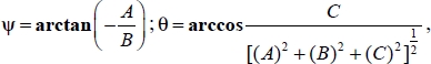

[2.6]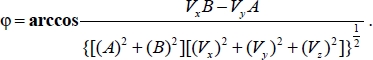

The components A, B and C of the normal vector to the reference plane are determined by the expressions

[2.7]

where x₀, y₀ and z₀ are the coordinates of a reference point that defines the space orientation of the target.

The position vector of the ijkth point scatterer with respect to the receiver, , is defined by

[2.8]

The round-trip distance from GPS transmitter to the target and from the target to the GPS receiver is defined by

[2.9]

The aforementioned analytical expressions can be used to describe the geometry and kinematic state of components of BGISAR scenarios and to model the BGISAR signals, as well as to implement image reconstruction procedures.

2.2. Multistatic BSAR geometry and kinematics

Consider the three-dimensional (3D) multistatic BSAR scenario presented in Figure 2.2 [MIN 12].

It comprises a satellite transmitter defined by current position vector R^s(p) in discrete time instant p, receivers defined by current position vectors and and a target of interest defined in a coordinates grid, all situated in a Cartesian coordinate system Oxyz. The target is presented as an assembly of point scatterers defined by coordinates in the same Cartesian coordinate system as the transmitter and the receivers.

Figure 2.2. 3D geometry of a BSAR scenario

Denote by R^s_ijk (p) the current range vector measured from the satellite transmitter with the current vector position R^s(p) = [x^s (p), y^s (p), z^s (p)]^T to the ijkth point scatterer of the target at the discrete moment p that can be described by the following vector equation:

[2.10]

where is the current position vector of the satellite transmitter, R^s(0) is the distance vector of the transmitter at the moment p = (N/2), is the vector velocity of the satellite transmitter, V = [V_x, V_y ,V_z]^T is the target vector velocity, T_p is the pulse repetition period or CW segment repetition period, N is the full number of emitted pulses or number of segments from emitted CW waveforms, R_ijk = [x_ijk, y_ijk, z_ijk]^T is the position vector of the ijkth point scatterer from a target with discrete coordinates x_ijk = i.ΔX, y_ijk = j.ΔY and z_ijk = k.ΔZ.

The current distance vector coordinates of the vector R^s_ijk (p) from the satellite transmitter to the ijkth point scatterer can be calculated by the following equations

[2.11]

where

[2.12]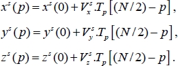

The module of R^s_ijk (p), the distance from the satellite transmitter to the ijkth point scatterer is defined by

[2.13]

Denote by and the position range vectors of two receivers, respectively. Then, the distance vectors target-receivers can be defined by vector equations

[2.14]

The projection of two vector equations onto Oxyz coordinate axes yields the following scalar equations for the determination of the ijkth point scatterer coordinates with respect to the first receiver (1) and second receiver (2):

[2.15]

[2.16]

[2.17]

where

[2.18]

The modules of and , the distance from the ijkth point scatterer to both receivers is defined by the following expressions:

[2.19]

[2.20]

Round-trip distance transmitter-ijkth point scatterer-first receiver can be expressed as

[2.21]

Round-trip distance transmitter-ijkth point scatterer-second receiver can be expressed as

[2.22]

Analytical expressions derived in section 2.2 can be used to describe the geometry and kinematic state of components of multistatic BSAR scenarios and to model multistatic BSAR signals as well as to implement image reconstruction procedures.

2.3. BFISAR geometry and kinematics

Assume that a stationary transmitter and a receiver are both located on the land or the sea surface and as, a mariner target, a ship – all situated in Cartesian coordinate system Oxyz. The BFISAR geometry and current kinematic state are shown in Figure 2.3 [LAZ 12a, LAZ 12b].

Figure 2.3. BFISAR geometjy

The target presented as an assembly of reflective point scatterers is depicted in its own Cartesian coordinate system O′XYZ. The vectors and are the position vectors of the transmitter and receiver, respectively, in a coordinate system Oxyz. The vector R_ijk = [X_ijk, Y_ijk, Z_ijk]^T is the position vector of ijkth point scatterer in a coordinate system O′XYZ and R₀₀ (p) is the current position vector of the mass center of the target at the time instant p. Based on the geometry in Figure 2.2, the following kinematic vector equations can be written:

[2.23]

where V is the target velocity vector, N is the full number of emitted pulses and T_p is the pulse repetition period or CW segment repetition period.

[2.24]

[2.25]

where A is the coordinate transformation matrix. If the axes O′Z and Oz are collinear,

[2.26]

where α is the vector velocity guiding angle defined between O′X and Ox axes.

– The distance vector from the ijkth point scatterer of the target to the receiver:

is defined by the expression

[2.27]

The main geometric feature of the synthetic aperture imaging is the module of the distance transmitter-target ijkth point scatterer-receiver defined by the expression

[2.28]

Analytical expressions derived in this section can be used to describe the geometry and kinematics of BFISAR scenarios and model multistatic BFISAR signals as well as to implement image reconstruction procedures.

2.3.1. Kinematic parameter estimation

Based on BSAR measurements, current distance and vector velocity of the target can be calculated. Assume that a point target moves rectilinearly at a constant velocity V along an arbitrary oriented trajectory. Distances R₀, R₁, R₂, R₃ , etc., from the receiving point B to the current positions of the point target can be measured at each moment p. The geometry of the target velocity estimation is presented in Figure 2.4, where V.T_p is the displacement of the point target along the trajectory for a period of measurements T_p.

Figure 2.4. Tajget velocity definition

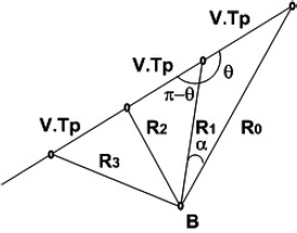
Applying a cosine theorem to two adjacent rightmost triangles and a sine theorem to the rightmost triangle in Figure 2.4, the following equations for the calculation of the target’s linear velocity and angle θ between the trajectory line and mass center line of sight can be defined:

[2.29]

[2.30]

where V is the linear velocity of the point target and T_p is the time interval of measurements.

Equation [2.30] can be modified; then, the time varying angle θ(t) between the trajectory line and mass center line of sight can be expressed as follows:

[2.31]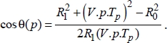

The azimuth angle between two consecutive azimuth directions for each p can be calculated by the following expression:

[2.32]

In conclusion, it has to be noted that the analytical geometrical approach is a powerful mathematical instrument for the description and modeling of a large variety of geometries and kinematics of components of BSAR scenarios. Mathematical expressions derived can be used to describe the geometry of objects of complicated shape, arbitrary oriented rectilinear trajectories and the kinematic state of the target, transmitter and receiver, as well as to calculate instant transmitter-target-receiver distances necessary to define the round-trip delay between the aforementioned components of the BSAR topology.