3

BSAR Waveforms and Signal Models

In this chapter, BSAR waveforms and signal models are presented. Short pulse signals, linear frequency modulated (LFM) and phase code modulated (PCM) waveforms and GPS (Global Positioning System) signal waveforms are some focus areas. Emphasis is put on the class of deterministic BSAR signals with wide bandwidth, such as short pulse signals, LFM signals, GPS and digital video broadcast terrestrial (DVB-T) signals, and low level of side lobes, such as Barker phase codes, complementary phase codes and GPS coarse/acquisition (C/A) and GPS precision (P) phase codes.

3.1. Short pulse waveform and the BSAR signal model

3.1.1. Short pulse waveform

Assume that the target is illuminated by a sequence of short monochromatic pulses, each of which is described by

[3.1]

where

In the above equation, A is the amplitude of the emitted signal; is the angular frequency; f is the carrier signal frequency; t = (m – 1)ΔT is the discrete current time, m = 1, 2, … is the number of current time samples, is the time duration of the signal sample, M is the full number of samples for a period of the carrier signal (1/f) and c = 3.10⁸ m/s is the speed of the light in vacuum; λ is the wavelength of the signal; and T is the time duration of the emitted pulse.

The sequence of short pulses is described by the expression [LAZ 11a]

[3.2]

where

t = mod T_p denotes the current time and = t – p.T_p denotes the fast time. For if t = p.T_p, then p = p + 1.

3.1.2. Short pulse BSAR signal model

For , the signal reflected by the ijkth point scatterer can be written as [LAZ 11a, LAZ 12a]

[3.3]

In the above equation, is the round-trip time delay transmitter-ijkth target point scatterer-receiver of the signal reflected from the ijkth point scatterer; a_ijk denotes the magnitude of the three-dimensional (3D) discrete image function, the intensity of the ijkth point scatterer; and t = mod T_p is the current time, where p denotes the number of emitted pulses, T_p is the pulse repetition period, = t – pT_p is the fast time, which in a discrete form is defined as t = (k – 1).T, k = 1, 2, … is the number of range cells where the BSAR signal is registered. The number of range resolution cells is calculated in accordance with the BSAR geometry described in Chapter 5, i.e.

[3.4]

where L is the length of the baseline, which is the distance between the transmitter and the receiver, and R_ijk (p) is the round-trip distance transmitter-ijkth target point scatterer-receiver. For each pth emitted pulse, the discrete demodulated BSAR signal from the target area recorded on radar rage resolution cells can be expressed as [LAZ 12d]

[3.5]

Equation [3.5] is a weighted complex series of finite complex exponential base functions. It can be regarded as an asymmetric complex transform of the 3D image function a_ijk, defined in a whole discrete target area into two-dimensional (2D) signal plane .

3.1.3. Target’s parameters estimation in short range BFISAR scenario

Consider a point-like target or a dominated point scatterer from the target illuminated by a meander-like pulse sequence. Then, having the reflected signal , the phase of this signal can be expressed as

[3.6]

where Re() and Im() are the real and imaginary parts of the complex signal, respectively.

The instrumental signal phase varies in the interval (–π/2) to (π/2). To calculate the instant distance to the point target, evaluation of the unwrapped phase of the received signal is required. After a standard unwrapping procedure over the measured Φ(p), the instant pseudo-distance between the target and receiving point can be expressed as

[3.7]

where p is the particular moment of measurement and is the unwrapped instant phase.

Having R_p, the target’s parameters, a linear velocity V and azimuth angles α can be calculated by expressions [2.28] and [2.31].

3.2. LFM pulse waveform

Assume that the object is illuminated by a sequence of LFM waveforms, each of which is described by

[3.8]

where is the angular frequency; f is the carrier frequency, c = 3.10⁸ m/s is the speed of the light; λ is the wavelength of the signal; t = (k – 1).ΔT is the discrete current time, is the index of the current time sample, T is the full number of samples in the pulse, is the time length of the sample, T is the time duration of an LFM pulse; and is the LFM rate. The bandwidth 2.ΔF of the transmitted pulse provides the dimension of the monostatic SAR range resolution cell ΔR = c/2.ΔF.

The sequence of LFM pulses is described by the expression

[3.9]

where t = mod T_p denotes the current time and = t – pT_p denotes the fast time; is the index of the emitted LFM waveform; and N is the full number of emitted LFM pulses. For if t = p.T_p, then p = p + 1.

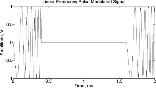
In Figure 3.1, the LFM pulse waveform is presented with the following parameters: f = 10⁵ Hz, T = 4.10^–4 s, and ΔF = 2.10⁴ Hz (Chapter 7, section 7.4).

Figure 3.1. LFM pulse waveform

3.2.1. LFM BSAR signal model

For each pth LFM emitted pulse, the deterministic component of the BSAR signal, reflected by the ijkth point scatterer of the target, has the form

[3.10]

In the above equation, a_ijk is the reflection coefficient of the ijk th point scatterer, a 3D image function; is the round-trip time delay of the signal reflected by the ijkth point scatterer; t = t_ijkmin(p) + (k – 1).ΔT is the current fast time, where is the sample index of an LFM pulse; number of samples of the LFM pulse, where ΔT is the time duration of an LFM sample; is the number of the radar range bin where the signal, reflected by the nearest point scatterer from the target, is detected, is the minimal round-trip time delay of the BSAR signal reflected by the nearest point scatterer of the target; K(p) = k_ijkmax(p) – k_ijkmin(p) is the relative time dimension of the target; is the number of the radar range bin where the signal, reflected by the farthest point scatterer of the target, is detected; is the maximum round-trip time delay of the BSAR signal reflected from the farthest point scatterer of the target.

The deterministic component of the BSAR signal is the superposition of signals reflected by all point scatterers placed on the target [LAZ 11c], i.e.

[3.11]

Demodulation of the BSAR signal return performed by multiplication with a complex conjugated emitted waveform yields

[3.12]

Equation [3.12] can be interpreted as a space transformation of the 3D image function a_ijk into the 2D BSAR signal plane (p, k) .

3.3. CW LFM waveform and modeling of deterministic components of BSAR signal

Assume that the target is illuminated by continuous wave linear frequency modulated (CW LFM) waveform, defined by the expression

[3.13]

where is the angular frequency, f is the carrier frequency, is the LFM rate, ΔF is the bandwidth of the transmitted pulse that provides for the dimension of the monostatic radar range resolution cell, i.e. ΔR = c /2.ΔF, t = (k – 1).ΔT is the current time, T is the half-time period of the triangle modulating pulse, is the index of the sample in a CW LFM signal segment; K is the full number of samples in the CW LFM signal segment measured on the range direction, ΔT is the time duration of an LFM sample and m is the number of the half-time period of the triangle modulating pulse.

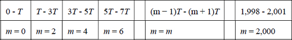
The parameter m accepts increasing even values in the following time instant intervals.

Table 3.1. Values of parameter m in time

The triangle exciting voltage and CW LFM waveform limited in the time interval from t = 0 to t = 4T, are presented in Figures 3.2 and 3.3, respectively, with parameters T = 10 ms, f = 2.4 × 10⁵ Hz and ΔF = 2.10⁴ Hz.

Figure 3.2. Triangle exciting voltage T = 10 ms

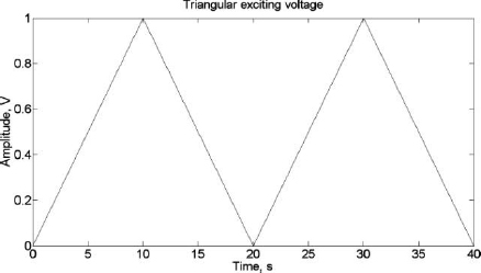
Figure 3.3. CW LFM waveform in the time interval from t = 0 to t = 4T

The deterministic component of the CW LFM BSAR signal reflected from the ijkth point scatterer can be expressed by

[3.14]

The deterministic component of the CW LFM BSAR signal reflected from all point scatterers of the target can be written by the expression

[3.15]

where a_ijk is a 3D image function, which is the reflection coefficient (intensity) of the ijkth point scatterer from the target; is the round-trip time delay of the signal from the ijkth point scatterer of the target.

CW LFM BSAR signal formation [3.15] can be considered as a direct projective operation of the 3D image function a_ijk onto (p, k) signal plane.

3.4. Phase code modulated pulse waveforms

Assume that a satellite transmitter illuminates a target by a phase PCM sequence during the coherent processing interval (CPI). Each phase code modulated waveform can be described by the expression

[3.16]

where A is the amplitude of the transmitted pulses, ω = 2πf = 2πc/λ is the signal angular frequency, φ₀ is the initial phase of the PCM pulse, t = (k – 1)ΔT is the current time, is the index of the PCM phase pulse (chip) and the full number of phase pulses (chips) in the PCM waveform.

The sequence of PCM waveforms in the case of φ₀ = 0 can be expressed as

[3.17]

where t = mod T_p denotes current time and = t – p.T_p denotes the fast time; p is the index of the emitted PCM waveform; T_p is the PCM pulse waveform repetition period in the case of Barker’s PCM pulse waveform or the segment repetition period in the case of CW PCM waveform. If t = p.T_p, for , p = p + 1.

3.4.1. Barker phase code

The parameters of Barker PCM pulse waveform are as follows: the number of phase pulses (chips) in Barker’s PCM waveform K = 13, the time duration of Barker’s PCM pulse waveform T and the time duration of the phase pulse (chip) ΔT that defines a monostatic radar range resolution. In Figure 3.4, a 13-element (chips) Barker PCM waveform is presented.

Figure 3.4. A 13-element (chips) Barker phase code modulated waveform

The time sequence of Barker’s phase code parameter b(t)can be presented as

[3.18]

3.4.2. Complementary code synthesis

Basic complementary code sequences empirically derived with ideal autocorrelation functions and zero side lobes are suggested in [BED 03]. The synthesis of complementary codes with unlimited length requires the creation of an initial first couple of codes with dimension n and a second couple of codes with dimension r.

The first couple of codes, presented as row vector matrices, has the form:

[3.19]

The second couple of codes, presented as row vector matrices, has the form:

[3.20]

To generate the elements of new codes with unlimited length, two algorithms can be applied:

Algorithm 1:

[3.21]

Algorithm 2:

[3.22]

The symbol (*) in the above formulas denotes a complex conjugate value.

3.4.3. BSAR-transmitted complementary phase code modulated waveforms

Assume that the BSAR transmitter emits two independent sequences of complementary PCM waveforms, each of which is described by the following expressions:

[3.23]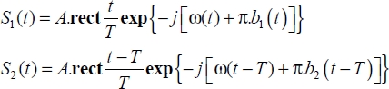

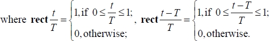
The sequence of two consecutive PCM complementary waveforms with pulse repetition period T_p can be written as

[3.24]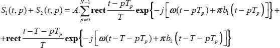

In the above equation, ω = 2π.f = 2π.c/λ is the signal angular frequency; t = (k – 1).ΔT is the discrete current time, where is the index of the phase pulse (chip) of the transmitted complementary PCM waveform; and is the full number of phase pulses in each part of the transmitted complementary PCM waveform, where ΔT is the time duration of the phase pulses of the complementary PCM waveform, T is the time duration of each part of the complementary PCM waveform and is the dimension of the range cell. For each PCM complementary pair and , the phase sign parameters b₁ and b₂ are defined as follows [LAZ 09]:

[3.25]

[3.26]

The phase sign parameters b₁ and b₂ are also described as follows:

[3.27]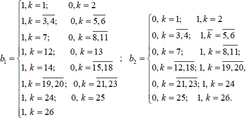

3.4.4. phase code

In the case of the application of GPS C/A PCM CW waveforms for BSAR purposes, the parameters of the GPS C/A PCM CW waveform need to be considered. These parameters are as follows: wavelength λ = 19.1 × 10^–2 m (carrier frequency f = 1.57.10⁹ Hz), registration time interval (segment repetition period) T_p = 2,2.10^–3 s, GPS C/A code repetition frequency of phase pulses (chips) 1.023 MHz and respective time duration of the C/A phase pulse ΔT = 0.9775.10^–6 s, time duration of GPS C/A PCM segment T = 10^–3s; full number of GPS C/A phase chips K = 1023, number of transmitted GPS C/A code segments during aperture synthesis N = 1024. A 30-element (chips) GPS C/A PCM waveform is presented in Figure 3.5.

Figure 3.5. A 30-element GPS C/A phase code modulated waveform

The tapped feedback shift registers (TFSRs) are used to generate a sequence of 0s and 1s of the phase parameter b(t) of the C/A (coarse acquisition) code at clock rate of 1.023 MHz (Figure 3.6).

At each clock pulse, the bits in the registers are shifted to the right where the content of the rightmost register is read as output. A new value in the leftmost register is created by the modulo-2 addition (or binary sum) of the contents of a specified group of registers [RAO 09 LAZ 11b].

Two 10-bit TFSRs are used, each generating a gold code:

– Code G₁ is presented as the polynomial: 1 + X³ + X¹⁰.

– Code G₂ is presented as the polynomial: 1 + X² + X³ + X⁶ + X⁸ + X⁹ + X¹⁰.

The output of the G1 (rightmost register) is modulo-2 added to the register contents of the G2. Different combinations of the outputs of the registers of G2 (or “taps” from the register) when added to the output of the G1 code lead to different pseudo-random noise (PRN) codes.

Figure 3.6. GPS C/A code generation

There are 36 unique codes that can be generated in such a manner. For example, PRN1 taps the contents of registers 2 and 6, and adds them to the output of the G1 TFSR; PRN2 taps the contents of registers 3 and 7; and PRN3 taps the contents of registers 4 and 8; and so on. Corresponding to the figure above, tap 1 is used in the numerical experiments (Chapter 7, section 7.6).

3.4.5. GPS Pphase code

In the case of the application of GPS P PCM CW waveforms for BSAR purposes while signal modeling, the parameters of the GPS P PCM CW waveform have to be taken into account. Consider a GPS transmitter illuminating a target with a segment of K-chips (phase pulses) of GPS P PCM waveform. Then each P PCM segment can be expressed by [3.16], where T = 13/(10.23 × 10⁶) s is the time duration of the segment and b(t) is the binary time sequence that modulates the phase of the GPS signal. For example, (K = 13)-chip segment b(t) may accept values 1001001001000.

The structure of a 30-element (chips) GPS P PCM waveform is presented in Figure 3.7. Matlab implementation is presented in Chapter 7, section 7.8.

Figure 3.7. A 30-element GPD P phase code modulated waveform

The GPS transmitter emits P (precision) code sequence on a carrier frequency L₁ = 1,575.42 MHz with a chipping rate of 10.23 × 10⁶, and a period of 6.1871 × 10¹² chips, generated by four 12-bit shift registers designated by polynomials X1A, X1B, X2A and X2B. The function of the registers is described by the polynomials as follows [FAR 93, LAZ 13]:

The initial states of the registers are as follows:

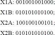
The GPS P code is a PRN sequence generated using four 12-bit shift registers designated X1A, X1B, X2A and X2B (Figure 3.8). The X1A register output is combined by an EXOR circuit with the X1B register output to form the X1 code generator and the X2A register output is combined by an exclusive-or circuit with the X2B register output to form the X2 code generator. The composite X2 result is fed to a shift register delay of the SV PRN number in chips and then combined by an exclusive-or circuit with the X1 composite result to generate the P code. X1A and X2A are both reset after 4,092 chips, eliminating the last three chips of their natural 4,095 chip sequences. The registers X1B and X2B are both reset after 4,093 chips, eliminating the last two chips of their natural 4,095 chip sequences. This results in the phase of the X1B sequence lagging by one chip with respect to the X1A sequence for each X1A register cycle. As a result, there is a relative phase precession between the X1A and X1B registers. At the end of each X1A epoch, the X1A shift register is reset to its initial state. At the end of each X1B epoch, the X1B shift register is reset to its initial state. At the end of each X2A epoch, the X2A shift register is reset to its initial state. At the end of each X2B epoch, the X2B shift register is reset to its initial state [RAO 09].

With the chipping rate of 10.23×10⁶, this sequence has a period of 26,641 days or 38,058 weeks.

Figure 3.8. GPS P code generation

The transmitter’s signal power is –163 dBW, and the receiver’s peak power is –120 dBm. Signal power density of the satellite transmitter on the Earth is 3.0628 × 10^–14 W/m². The receiver-to-target range varies in the interval 100–1,000 m.

The deterministic component of the PCM BSAR signal reflected by the ijkth point scatterer is defined by

[3.28]

where a_ijk is the 3-D image function that defines the intensity of each ijkth point scatterer; T is the time duration of the phase code sequence, is the round-trip delay from the ijkth point scatterer; t = t_ijkmin(p) + (k – 1).ΔT is the current time, ΔT is the time duration of the phase segment, is the current number of segment, K = T/ΔT = 1023 is the full number of segments of the C/A phase code, is the relative dimension of the target, and are minimal and maximal round-time delays, respectively.

The deterministic component of the BGISAR signal, reflected by all point scatterers of the object for every pth phase code pulse sequence, has the form

[3.29]

For computing rect[t – t_ijk(p)/T] time delays, t_ijk(p) are arranged in ascending order. An index different from this order is introduced in the definition of t_ijk(p), i.e. . Then equation [3.29] in discrete form can be rewritten as

[3.30]

where denotes the current number k while rectangular function, , for a particular t_ijk(p) accepts value 1 first time and can be considered as a projective discrete coordinate of the ijkth point scatterer on the range direction. It is possible for a large number of time delays, t_ijk(p) the rectangular function to accept value 1. Equation [3.30] can be used to model the PCM BSAR signal reflected from the target.

3.4.6. DVB-T waveform

DVB-T is the digital television broadcast system used in many European countries. Assume that the target is illuminated by the signal emitted by DVB-T system that uses a digital coding modulation of the signals in order to propagate many TV programs. The DVB-T signal can be expressed as [CHR 09]

[3.31]

where

where k is the carrier number, l is the orthogonal frequency division multiplexing (OFDM) symbol number, m is the transmitter frame number, K is the number of transmitted carriers, T_s is the symbol duration, T_u is the inverse of the carrier spacing, Δ is the guard interval, ω_c = 2π.f_c is the central angular frequency of RF signal, k′ is the carrier index relative to center frequency, , and c_m,l,k is the complex symbol for carrier k of the data symbol number l in frame number m.

The signal reflected from the moving target will have the form

[3.32]

where

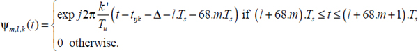
Table 3.2. Parameters in the Norwegian DVB-T system

In conclusion, it is worth noting that the spectrum and respective tie duration of the emitted waveforms defines the range resolution of the BSAR system. Wideband spectrum waveforms as short pulses, LFM waveforms, Barker PCM waveforms, GPS C/A and GPS P phase modulated waveforms are applied to achieve a high range resolution. Based on the geometry and high informative waveforms, a mathematical description of the BSAR signal, reflected by targets of complicated shape, is given and interpreted as a direct space transformation of the 3D target image function into the 2D signal function or a 3D image of the target into a 2D signal plane.