
This chapter is about …
What spreadsheets are and what they can do. All of the principal facilities and functions needed to create and use the forecasting models in the book are explained here, with examples of their use. There is also a section of handy tips and shortcuts.
How to use the example files
This part of the book will introduce the practical use of spreadsheets. Where reference is made to one of the downloaded examples it is shown as EXnn, where nn is the example number. These relate to the numbers on the tabs at the foot of a spreadsheet.
Microsoft Excel™ is the spreadsheet we’ll use throughout the book and for the downloaded examples, but other types will probably have identical or at least very similar features.
We will only need to use a very small proportion of the features available in Excel, and there are usually several different ways of doing the things described. For example there are a number of ways of copying and pasting formulae, and the ones that I use aren’t better or worse than any other. If you are already familiar with Excel and are used to doing things in a different way to that described, stick with what you know.

Excel has very good help features if you get stuck. If there’s something that you want to do, then in all probability there is a way of doing it.
There is one piece of advice that is applicable to all computer programs: READ THE SCREEN. Yes, it is obvious, isn’t it? But it’s amazing how quickly we forget the obvious when presented with a new screen. We look, but don’t see and read it. More often than not somewhere on the screen, perhaps in the mouse rollover text on toolbar icons, you are told what your options are or how to put them on the screen. So, look carefully and have a play around to see what’s available.
What are spreadsheets?
Spreadsheets are closely analagous to a simple principle that can be easily explained with pencil and paper. Let’s take a few columns of figures, with totals at the bottom of each one – see Figure 3.1. This shows that, for example, 293 = 16 + 4 + 273.

Now put some labels on each of the rows and columns, so that each intersection of a column and row can be given a unique identity – see Figure 3.2. The spaces at the points of intersection of the rows and columns are called cells.
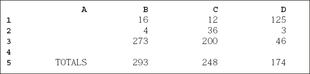
For example, the number ‘4’ is in cell B2. This description of a cell’s position is called its address.
Similarly, the numbers ‘16’ and ‘273’ are in cells B1 and B3 respectively, and the sum of them all, ‘293’, is in cell B5.
Now, if the figures are replaced with their cell names, the sum can be expressed as in Figure 3.3.
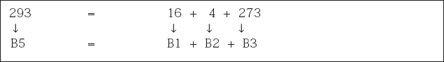
And this is precisely and simply how a spreadsheet works. Figures can be placed in the cells, in exactly the same way as in the paper example. The big difference is that wherever a calculation is needed, the spreadsheet will automatically carry it out when it’s entered in the cell where the answer is required.
For example, in Figure 3.3, if the calculation ‘=B1+B2+B3’ is entered in cell B5, the result ‘293’ will appear in cell B5.
And what’s more, if the figure in any cell referred to by cell B5 is changed, say you replace the ‘4’ in cell B2 with ‘50’, the new result ‘339’ would immediately appear in cell B5.
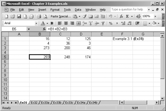
In Example 3.1 later (see page 41) you can see the columns and row border labels, and a replica of the table. The bold rectangle on cell B5 is the ‘cursor’ – but more of this later. I have placed the cursor here so that you can see the contents of the cell. It appears near the top of the screen as =B1+B2+B3 and is the calculation that gives the result 293.
The position of the cursor can also be seen in another way. At the top left of the screen is B5, which is the cursor’s position.
OK – so what’s all the fuss about if that’s all spreadsheets can do? Well of course, they will do very much more, but the principles are exactly the same: figures, or calculations (formulae) expressed in terms of cell addresses, or both, can be entered in any cell.
The results of formulae will always reflect exactly any changes made in cells referred to by them.
Examples of principal facilities and functions
This section summarises the most significant functions and capabilities of spreadsheets. You’ll use most of them in Chapter 4 when you work through building the example models.
The subjects covered here are:
- spreadsheet size;
- the cursor, and moving around the spreadsheet;
- entering numbers and text;
- column width;
- basic arithmetic;
- copying cell contents;
- functions;
- copying a function;
- absolute addresses;
- copying absolute addresses;
- inserting and deleting rows and columns;
- formatting the presentation;
- charts (graphs);
- ranges;
- naming ranges.
Spreadsheet size
Excel has 256 columns (A – IV) and 65,536 rows available. This is far more than you are likely to need for your budget and forecast.
The cursor, and moving around the spreadsheet
The cursor has two purposes; firstly it allows you to select a cell to make changes to it, and secondly to use it as a ‘pointer’ to move around the spreadsheet. Normally only about 20 to 30 rows and 8 to 12 columns can be seen on the screen at any one time, but scrolling up and down, or left and right, reveals any other part of the spreadsheet.
The cursor can be moved in a number of ways:
- using the keyboard ‘arrow’ keys
 to move one cell at a time in the direction indicated;
 - using the keyboard PgUp (Page up) and PgDn (Page down) keys to move a screen height at a time, up or down;
- and of course by using a mouse.
Entering numbers and text
Numbers, calculations, cell addresses, text and special functions can be put into any cell by simply placing the cursor on the cell where they are required, typing them, and pressing the Enter key.
Putting an equals sign ‘=’ prefix in an entry tells Excel that it is for a calculation, whereas plain text should be entered without it.
Note: In the book, characters that are to be entered are in bold text.
Try moving the cursor around, and changing some numbers, or entering some new ones on Example 3.1 (Ex31).
Column width
The width of a column is described by the number of characters or figures it can contain. Each column width can be set to accommodate as many figures or characters as necessary. If the cells to the right of a cell that contains text are empty, any characters more than the width of the cell will simply spill over.
Basic arithmetic
Calculations using addition, subtraction, multiplication and division are entered exactly as they would be written on paper, using the keyboard symbols + – * / respectively.
Basic arithmetic can be entered as:
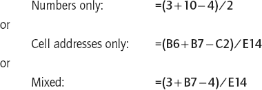
Copying cell contents
Spreadsheets very often need calculations in several places that are identical in form, but which refer to different cells. For instance, in Example 3.1 (Ex31) the calculations for the totals from left to right are =B1+B2+B3, =C1+C2+C3 and =D1+D2+D3. Now, while it’s easy to individually enter these three calculations, it would be very time consuming and tedious to type and enter them across a large number of columns.
Spreadsheets have a copying facility so the contents of a cell can be copied as many times as needed, and what’s more, by default any cell addresses they contain are automatically adjusted during the copying process.
So if, for instance, in Example 3.1 (Ex31) the ‘Totals’ calculation was also wanted in cells E5 to H5, just instruct the spreadsheet to copy the contents of cell D5 into the range E5 to H5, and the correct changes to the formulae will be automatically made. The contents of cells E5 to H5 will then be =E1+E2+E3, =F1+F2+F3, =G1+G2+G3 and =H1+H2+H3 respectively.
There are different ways to copy the contents of cells, using the example above:
- Put the cursor on D5, click the copy icon on the tool bar, put the cursor on E5 holding the left mouse button and drag it over F5, G5 and H5, then click the paste icon on the tool bar.
- Put the cursor on D5, use Ctrl+C or Ctrl+Ins to copy, using the right arrow key move the cursor to E5, hold the shift key down and use the right arrow key to highlight F5, G5 and H5, then press Enter to paste. (This is the method I use, finding it quicker and more accurate than using the mouse.) You can also use Ctrl+V to paste.
- Put the cursor on D5 (see that the bottom right-hand corner of the bold outline has a small black square), and using the mouse, position the cursor exactly on the small black square (the cursor will change to a + ); left click and drag over E5 to H5 then release the mouse button.
Ex31: Copy cells D5 to E5:H5, and try entering numbers in any or all of cells E1, E2, E3, F1, F2, F3, G1, G2, G3, H1, H2, H3 to see that they are picked up by the formulae.
Functions
Excel provides many ready-made functions, designed to simplify and minimise your work constructing commonly used calculations and those for very specific purposes (see Table 3.1).
Table 3.1 Some Excel function categories
- Financial
- Math and Trig
- Lookup and Reference
- Text
- Information
- Date and time
- Statistical
- Database
- Logical
Most of the functions are not required for budgeting and forecasting, but it’s worth mentioning examples from the main categories to give you some idea of what’s available.
Financial
| NPV | Net present value |
| SLN | Straight-line depreciation for one period |
Date and time
| NOW | System date and time |
| DATE | Date value of a specified date |
Math and Trig
| SUM | The arithmetic sum of a range |
| SQRT | Square root of a value |
| ROUND | Value rounded to number of decimal places |
| SIN | Sine of a value |
| PI | Gives the value of Pi (π) |
Statistical
| AVERAGE | The average of values in a range |
| COUNTBLANK | The number of blank cells in a range |
Lookup and reference
| CHOOSE | Choose a value or action |
| LOOKUP | Look up a value in a column or row |
Database
| DCOUNT | Number of cells containing specified numbers |
| DMAX | The largest number matching a specified condition |
Text
| RIGHT | Last n characters of text string |
| LEN | Length (in characters) of a text string |
Logical
| IF(x,y,z) | If x is true then y, otherwise z |
| OR(x,y) | True if either x or y is true, otherwise false |
| AND(x,y) | True if both x and y are true, otherwise false |
Information
| ISNUMBER | True if value is a number, otherwise false |
| ISTEXT | True if value is text, otherwise false |
One of the most commonly used functions is SUM, and so it’s a helpful one to look at more closely in a practical illustration.
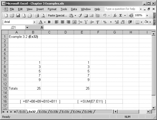
Consider two columns of five figures in cells B7 to B11 and E7 to E11 that require totalling in cells B13 and E13, respectively.
One way to add the figures in column B is to type the calculation into B13 like this:
=B7+B8+B9+B10+B11
That will certainly work, and it wouldn’t take long to type it in as there are only five figures. But suppose you had 20 or even 100 figures – that would be an enormous amount of typing with a very high probability of error. The SUM function eliminates the need for all the typing, and has some other advantages as well which we’ll look at later.
SUM totals the contents of all of the cells within the range in its brackets, so putting =SUM(E7:E11) in cell E13 will give the same result as adding each cell individually.
Cell ranges are shown as the first and last in the series, with a colon between. For example, =SUM(E7:E11) means all of the cells within the range, in this case E7, E8, E9, E10 and E11.
Example 3.2 shows the two identical columns of figures. The formulae shown in square brackets are the contents of the totals in cells B13 and E13.
Note: Things in square brackets are just my explanatory notes, they are not part of the spreadsheet’s calculations.
Changes to any of the numbers in column E of Example 3.2 will still be reflected by the total =SUM(E7:E11) of course, in exactly the same way as the formula =B7+B8+B9+B10+B11 for column B totals.
Copying a function
Copying the formula =SUM(E7:E11) to other columns will, just as before, automatically adjust the cell addresses.
Copy SUM(E7:E11) from E13 to F13; it will adjust to SUM(F7:F11). Then put some numbers in F7 to F11 to see what happens.
Until now totals have been positioned at the bottom of columns of figures, but there is no reason why formulae should not be placed, or indeed repeated, anywhere. For example, suppose the totals for columns B and E in Example 3.2 were also wanted at the top right-hand of the screen, one above the other. This can be achieved by repeating the formulae for the totals, or by simply entering the cell addresses of where the totals are in the cell where they are required. The first way just repeats the calculations, the second displays whatever is in the cell referred to, and is probably the easiest and best method in most circumstances.
We’ll try both methods. For the first, there are two ways of repeating a formula elsewhere: either retyping the calculation at the new location or by copying it from the original location.
Copying is the very much easier and preferred way of course, but the automatic adjustment of cell addresses, when a formula is copied, must be inhibited. Excel has a way of creating or copying what are known as absolute addresses, that is, addresses that will not change or adjust to a new location under any circumstances.
We’ll look at absolute cell addresses in more detail before copying the totals to the top right of the screen.
Absolute addresses
The way in which an address can be made absolute looks a little complicated at first, but only because of the unfamiliar appearance of a $ symbol in a calculation. This has nothing whatever to do with currency, the $ symbol is just being used as an instruction in the addresses.
We’ll just recap on what happens when an address is copied from one location to another and the address is automatically adjusted. This is known as relative addressing, because the adjustment is based on the relative position of the new location to the old. Simply put, if a cell address is copied two columns to the right, the column part of the address will increase by two columns.
Thus if cell address B2 is used in a formula somewhere, and the formula is copied two columns to the right, the address B2 in it will increase by two columns, that is from B to D, making the new address D2. Similarly, if the same formula is copied two rows down, the address B2 will increase by two rows, from 2 to 4, making the new address B4. Finally, if the formula is copied to a location two columns to the right and two rows down, the address B2 will adjust to D4.
So, the default behaviour of Excel when an address is copied is relative addressing – the address column and row are automatically adjusted for the number of columns or rows from the original address that it is copied to.
An absolute address doesn’t change, wherever it is copied to. An address can be made absolute in respect of either its column, or its row, or both. Placing a ‘$’ before either the column or row part of a cell address makes that part absolute.
For instance, $B2 makes the column absolute, B$2 makes the row absolute, and $B$2 makes both the column and the row absolute.
Copying absolute addresses
- If the original address is $B$2, wherever it is copied to, it will still be $B$2.
- Or if the original address is $B2, the column ‘B’ will always remain the same, but the row ‘2’ will adjust relative to its new position.
- Or if the original address is B$2, the row ‘2’ will always remain the same, but the column ‘B’ will adjust relative to its new position.
It works in exactly the same way in ranges: SUM($B$2:$B$3) will be unaltered wherever it is copied to, and SUM($B$2:B3) will adjust only its second, B3, part.
Look at Example 3.3a (Ex33a). In H2 repeat the formula at B13, i.e. =B7+B8+B9+B10+B11, and enter =E13 at H3. Put the labels Total column B and Total column E in F2 and F3 respectively, to identify which is which.
Now whatever happens to the figures in column B and column E will be reflected by the totals at their foot, and at the top right of the screen in H2 and H3.
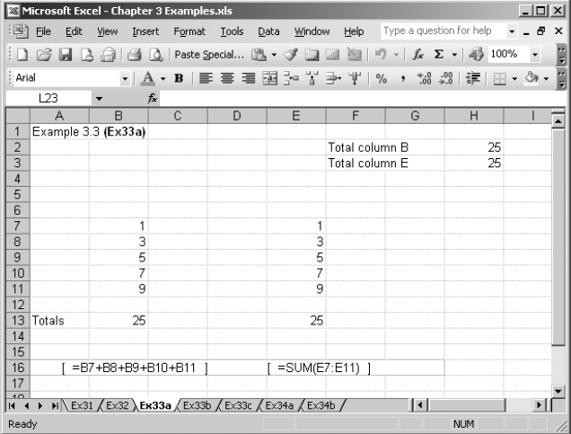
Example 3.3a (Ex33a) Two ways of repeating the column totals
Inserting and deleting rows and columns
There are all sorts of reasons for wanting to insert or delete rows and columns, not the least being errors or changes of mind, if my own experience is anything to go by! It is very easy to insert or delete rows and columns, after which the spreadsheet will automatically relabel the whole spreadsheet’s rows and columns so that they still run on in an unbroken numeric or alphabetical sequence. Furthermore, all existing cell addresses will also automatically and immediately adjust to their new locations.
Let’s see what happens if a new row is inserted above the existing row 9, in Example 3.3b (Ex33b ). So far so good – there is now an extra row, the rest of the rows have been renumbered accordingly, and the totals are still correct.
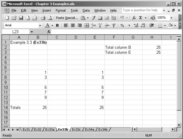
Example 3.3b (Ex33b) Inserting an extra row
But what if figures are now put into the newly created cells B9 and E9? Let’s put 100 into each B9 and E9 as shown in Example 3.3c (Ex33c). Now, what’s happened? The total for column E is correct, but the column B total hasn’t picked up the additional 100.
In Example 3.3c, looking at the total formula in B14 shows why this occurs. The spreadsheet has adjusted the formula to =B7+B8+B10+B11+B12, which doesn’t include the new row 9, because it hasn’t been told to include it.
But looking at the formula in E9, this has adjusted to =SUM(E7:E12), and this is another major advantage of using the SUM function. The last address in the range has adjusted, correctly of course, to E12. Clearly then, the new row 9 is included in the range E7:E12 and the sum is therefore still correct.
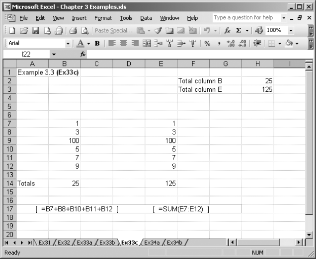
Example 3.3c (Ex33c) The effect of a new row on the different ways of adding a column of figures
So the SUM function enables additional rows and columns to be inserted whilst the integrity of their calculation is maintained. It also minimises the risk of unwittingly creating formulae that probably don’t do what is actually wanted, as in B14.
If Row 9 had been deleted instead, the SUM function in E14 would still have worked properly, but the ‘addition of individual cells’ version in B14 wouldn’t even have given an answer at all – it would have displayed an error message, such as #REF!
Looking at the formula would show that where B9 was you now have an error message, like this for instance: =B7+B8+#REF!+B10+B11.
Formatting the presentation
Formatting is concerned with the appearance of the display, both on the screen and when printed on paper. It has no effect whatever on the calculations.
There are several formatting facilities, of which one is column width, mentioned earlier. The rest are mainly concerned with the presentation of text (labels) and figures.

Justification refers to the presented position of the contents of a cell within it. Text, figures and the result of any calculation can be justified to the left or to the right, or centred within the cell. By default, text is left justified and figures are right justified. Whilst it’s rare that figure justification needs to be changed, it is frequently required for text. For example, if you wanted the abbreviated month labels – Jan, Feb, Mar and Apr – at the heads of their columns.
Example 3.4a (Ex34a) shows a sales forecast model for a number of salesmen. Note that column A has been widened to accommodate the labels.
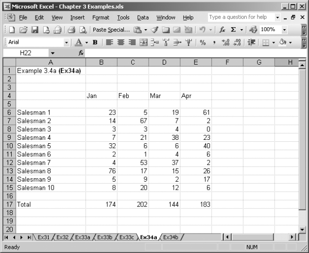
Example 3.4a (Ex34a) Month headings – left justified
There is no need to type in each of Salesman 1 to Salesman 10. Just type Salesman 1 where required, then use the black square at the bottom right of the cell outline when the cursor is on it to copy downwards, and the 1 will increment as you left click and drag it. This works for any text with a number at the end. Similarly, for the months just enter Jan (or January if you wish) and drag the black square to the required month. Excel automatically recognises that a sequence might be required.
I have put the month labels and figures in without changing any formatting arrangements, and they have defaulted to text left and figures right. There is so much misalignment between the month headings and the figures that it is quite difficult to see which belong to which, especially lower down the spreadsheet. The solution is to format the text headings to right justification. Formats can be applied to individual cells, or to an entire row or column. In this case, because row 4 will contain only headings, I’ll format the row to right justify and set as bold text.
In Example 3.4b (Ex34b) the headings are now properly aligned with the figures, and consequently much easier to read.
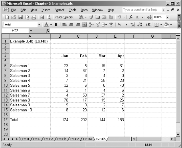
Example 3.4b (Ex34b) Month headings – right justified and bold
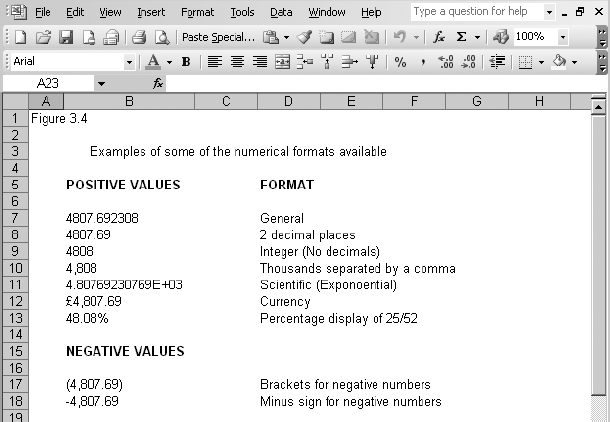
Numerical format refers to the way in which figures are displayed; remember, none of the following affects the accuracy of any calculations.
Suppose we have a calculation of 250000 divided by 52. That’s 250000/52, which is 4807.69230769 to eight decimal places. But it is unlikely in budget applications that a display like this would be wanted. We are more likely to require two decimal places, which is 4807.69 rounded down.
Just about any presentation can be produced on a spreadsheet – a selection is displayed in Figure 3.4. The column used for the figures is set to a width of 15 characters, and the figures themselves are left justified for clarity.
Charts (graphs)
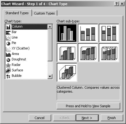
There are many instances in budgeting and forecasting when graphical representation of some of the figures can be very useful indeed. Figure 3.5 shows a screenshot of Excel’s Chart Wizard.
Ranges
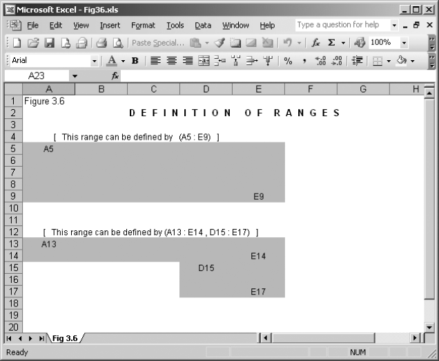
A range, as it was used for example in the SUM function, is a block of cells that can be fully defined by its top left-hand corner and its bottom right-hand corner – see the upper example in Figure 3.6. You can also combine two ranges and treat them as one for the purpose of functions – see the lower example in Figure 3.6.
Naming ranges
Ranges can be given names – literally any name you like. In Figure 3.7, the range in the upper example has been given the name SALES, and can then be referred to by name. So, instead of having to type SUM(A5:E9), SUM(SALES) can be entered. In fact, having named a range, even if you do enter it typed in full, the spreadsheet will immediately replace the range with its name.
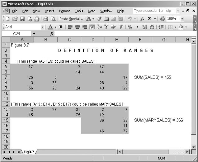
Figure 3.7 Spreadsheet named ranges
The main advantages of using named ranges are that formulae are easier to construct, and easier to understand later on. For example, if the sum totals of sales for the months of January to December are required in various calculations, each of the totals can be named JANSALES, FEBSALES, … etc. Thereafter, in any formula that requires them, instead of having to remember the addresses of the ranges, all you need to do is type the name(s). The first quarter’s sales could be calculated simply by typing JANSALES+FEBSALES+MARSALES.
Obviously any calculations that look like this will be much more easily understood by anyone else, and by you as well when you look at the spreadsheet again, in detail, for the first time 12 months later! Named ranges have saved many a scratched head and premature baldness.
Handy tips and shortcuts
If you’re an experienced Excel user you will have already established your own favourite shortcuts, and picked up a lot of the many handy bits that it has tucked away. If you’re not an experienced user, this section on handy tips and shortcuts might be useful to you. There’s nothing special about my list, it’s just the way I do things, but some of them could be useful to you.
Toolbars
Toolbars on Excel are (usually) at the top of the window, and populated with a number of shortcut tool icons – see Figure 3.8. The toolbars can be customised to include and exclude any tool icons that you wish.
Obviously it’s sensible to have those that you use the most.

To customise the toolbars, go to View / Toolbars / Customise. The Options tab has the basic settings, and on the Commands tab you can select which commands you want on the toolbars. Whilst the toolbars Customise dialogue window is open, unwanted icons can be dragged off the toolbar: just left click and drag an icon downwards until an X appears – release the mouse button and the icon has gone.
To add an icon to the toolbar, left click and drag an icon from the Commands tab of the Customise dialogue window to the position on the toolbar where you want it, and release the mouse button.
The toolbar icons I find particularly useful include:
- Paste special
- Format painter
- Insert function
- New Comment, Show/Hide Comment, Delete Comment
- Sort A-Z, Sort Z-A
- Chart wizard
- Drawing
- Zoom
- Font style and size, Bold, Italic, Underline, Colour
- Align Left, Centre, Right,
- Merge and Centre, Merge cells, Unmerge cells
- Increase decimal, Decrease decimal
- Insert Rows, Insert Columns, Delete Rows, Delete Columns
- Borders
- Fill colour.
Totals with the cursor
Have you noticed that whenever you highlight a cell, or many cells, their arithmetic total appears on the right-hand side of the status bar at the bottom of the Excel window?
Moving around with Ctrl + another key
Note: Ctrl + <another key> means use the Ctrl key and another key at the same time.
Some of these can be very useful on large spreadsheets:
- Ctrl + End – moves to the bottom right cell of the used area.
- Ctrl + Home – moves to the top left cell of the used area (within a frozen pane if there is one).
- Ctrl + Up arrow / Down arrow / Left arrow / Right arrow – moves in the direction of the arrow to the next populated cell, or if within a block of populated cells, to the end of that block.
Arrow keys instead of Enter
When a value is entered in a cell with the Enter key, the cursor will move in the direction, if any, that’s set in Tools / Options / Edit / Move selection after edit.
This will be set to your generally preferred direction, but at any time you can use one of the arrow keys, instead of the Enter key, to enter a value in a cell, and the cursor will move in the direction of the arrow.
Cell notes
Cell notes are a very handy way of making annotations and notes without any danger of affecting calculations or the normal behaviour of a cell. The size of the notes window can be adjusted as required, and it can be set to display all the time, or only when the mouse pointer is over the cell.
Paste special
The paste special options (see Figure 3.9) are available after copying something. The paste special dialogue window can be found under the Excel Edit menu, or if you have the Paste icon on your toolbar (recommended), Alt + S invokes it.
The default paste special option is ‘All’, which is the same as doing an ordinary paste.
Other Paste options include: pasting Formulas only (i.e. not formats or comments); values only (i.e. not formulas, formats or comments – this one I find very useful); formats only, which is the same as using the format painter; comments only; and various other characteristics that it might be useful to paste on their own.
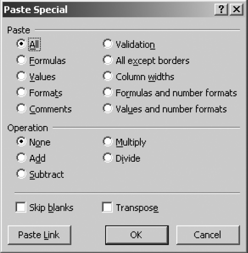
The ‘Operation’ options Add or Subtract simply Adds the value you are copying to the value already in the cell you are copying to, or Subtracts the values you are copying from the value already in the cell you are copying to. Similarly for the Multiply and Divide options.
Skip blanks can be used with any paste, and avoids replacing values in the paste area when blank cells occur in the copy area.
Transpose changes rows of copied cells to columns, and vice versa.
Summary
In this chapter we have:
- realised that computer spreadsheets work in a similar way to their paper equivalent;
- learned that the intersection of columns and rows is called a cell, and is described by a letter and number known as a cell address;
- devised calculations which can be written into cells, and include figures, cell addresses and formulae;
- done the same with explanatory or labelling text;
- seen that there is a huge range of functions available in a spreadsheet, some of which make model construction easier, and others that are more specialised.