
Appendix
Two-terminal modelling equations and spreadsheets
Whether we measure a capacitor, explicit inductor or a transformer winding’s leakage inductance, we are simply measuring the impedance of a combination of components between two terminals. We imply a model the moment we assign LCR component values to that impedance. Modelling accuracy invariably breeds model complexity, so this section aims to show you how to create and test spreadsheet models ranging from simple to complicated with an absolute minimum of pain.
Once we have a mathematical model of a component’s impedance, a spreadsheet can very easily calculate impedance at many different frequencies, plot the results as a graph of impedance against frequency, and overlay measured impedance against frequency. Iteratively adjusting model values the two curves are perfectly overlaid allows a component’s parasitic values to be determined, allowing more realistic and reliable modelling of entire circuits. But first we need that model…
Spreadsheets were developed for accountancy, not engineering, so they don’t handle complex algebra particularly well, and the way that equations have to be entered makes mistakes likely. However, breaking the problem into small steps allows simple equations that can be entered and checked easily. Obviously, LTspice can analyse and plot the response of a complex circuit with far less effort, but it can’t overlay your measured result for comparison, and that’s why we tolerate the clunkiness of a spreadsheet for generating component models. Thankfully, we only have to enter the equations for a particular model once. Thereafter, we rename our spreadsheet and enter new measured data for comparison.
We know we will produce a complex spreadsheet having many rows and columns, so rather than adjusting model values in their individual columns, we list our components at the top left of the spreadsheet and use absolute rather than relative addressing ($B$5, rather than B5) in the calculations needing to pick up component values. This makes it easy to adjust model values once the graph has been plotted.
Each reactive component needs its own column to calculate reactance at each frequency of interest. Thus:

Rather than neatly collecting these columns to the left of the spreadsheet, reactance columns are best added as each new component is introduced, keeping them close to the equations that use them.
No matter how many parasitic components there may be in total, a two-terminal problem can always be resolved into series and parallel combinations, but with the added difficulty that each step adds its single component (R, jXL, or −jXC) to a complex impedance (A+jB).
There are six possible situations:
Adding a series resistance:
![]() (A.1)
(A.1)
Adding a series inductance:
![]() (A.2)
(A.2)
Adding a series capacitance:
![]() (A.3)
(A.3)
Adding a parallel resistance:
![]() (A.4)
(A.4)
Adding a parallel inductance:
![]() (A.5)
(A.5)
Adding a parallel capacitance:
![]() (A.6)
(A.6)
Note that each of the six preceding equations is in A+jB form, so one column is required to calculate the A (real) term and another for the B (imaginary) term. If you have never understood complex numbers and treasure that ignorance, don’t panic. Quietly ignore the significance of “j”, but be aware that a complex number is composed of an A and jB term, that they are different, and may not be mixed. Think of them as apples and oranges, if you wish.
You will notice that the denominator (lower line) for the parallel equations is the same for the A and jB terms, so equation entry can be simplified by adding a third column for the denominator, then calculating the A and jB terms by entering the equation for the top line (numerator) and dividing it by the result already calculated in the denominator column. Further, you may notice that the parallel equations have been expressed in a way that highlights their very similar shape, making them easier to enter or check. Additionally, it is moderately easy to convert an inductance cell into a capacitance cell and vice versa, enabling copying and pasting followed by small edits, rather than entering everything individually in full.
Just like the DC resistive analysis described in Chapter 1 of Valve Amplifiers, we start analysis from as far away from the output terminals as possible, picking a point where we can combine just two components. We then work outwards towards the output terminals one component at a time, adding columns at each point to the spreadsheet. If we need to add both resistance and reactance in parallel, it does not matter in which order we perform the calculations, we can either enter the A+jB values from the resistance addition into the capacitance or inductance addition, or vice versa. If we later find that we want to modify the model and insert an extra component or two, we simply insert columns at the appropriate point and modify the next set of columns to pick up the appropriate result.
Once we have introduced all our components, the far right of our spreadsheet has a pair of columns describing the network’s impedance in A+jB form, but we need to convert into Z, Φ form because that is what our test jig measures:
![]()
And if we wanted the phase angle:
![]()
Once we have the magnitude of impedance (Z), we copy our cells down for as many frequencies as required, enter each individual frequency, and out will pop a calculated impedance that we plot against frequency (double-click on each axis and select a logarithmic scale). The graph of Z against frequency is very useful for checking equation entry, so if this is plotted early on, its A+jB to Z conversion columns can be temporarily set to pick up the A+jB result of each component addition and the graph inspected to see if it looks plausible. Thus, we might start with a series combination of inductance and resistance and plot their resulting impedance, expecting to see a graph with a horizontal line equal to the resistance, then a line rising with frequency for the inductance. If we then added parallel capacitance, we would expect to see a resonant peak, after which impedance would fall with frequency. We could even check the resonant frequency using:
![]()
Bear in mind that this simple resonance equation does not take account of the frequency pulling effect of resistive components, so provided the model equations suggest a resonant frequency within a few per cent of the simple resonance equation, they are right and the simple equation is wrong.
If we add a shunt resistance, we should expect to be able to adjust peak amplitude.
Once we have a plot of modelled impedance against frequency, we add the measured impedance against frequency to the graph and adjust model values until the two overlay. We use the measurement frequencies as input frequencies to our model because this allows perfect overlay for a perfect model. Useful tip: If you have a frequency counter (many DVMs include one) use this when you make the impedance measurement and enter the actual frequency (perhaps 1.0245 kHz) rather than the intended nominal frequency of 1 kHz; in this way, the model will calculate using the applied frequency, and compare like with like.
If we finally add a column to our calculations that divides modelled impedance by measured impedance, subtracts 1, and expresses the result as a percentage, we have the percentage discrepancy, and this can be linearly plotted against frequency (logarithmic scale), allowing model values to be fine-tuned for minimum discrepancy. If this graph uses the same frequency scale as the impedance graph and is positioned directly below it, glancing between the two makes it easier to identify which component value needs adjusting to minimise discrepancy.
Note that LTspice includes the four-component model as standard for its inductors and capacitors (although not resistors), and calculates more efficiently if this is used than if parasitic components are added externally. Obviously, if a six (or more) component model is required to describe a component, it will have to be entered as a collection of individual elements.
Once you have modelled a few components (inductances, especially), you will discover that it is possible to generate two models whose discrepancy graphs have very similar maximum variation (but entirely different shape), so which one is right? The answer is neither. There is no absolute right. What you have is a collection of components that behaves in a similar fashion over the tested frequency range. It is very dangerous to attempt to extrapolate over a wider frequency range unless you have an excellent physical understanding of the modelled component. Even then, it is far better to take extra measurements so that the comparison encompasses the working frequency range.
Assuming that the comparison covers a sufficiently wide frequency range, it can generally be said that a poor model produces many sharp variations in the discrepancy graph whereas a good model tends to have a smoothly varying discrepancy.
Six-component worked example
We want to model a 10 H HT choke using the split inductance model. See Figure A.1.
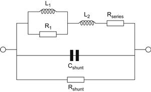
Figure A.1 This split inductance six-component model can describe a practical inductor quite accurately.
We have six individual component values, so we use cells 1–6 in column A to label them in order (L1, R1, L2, Rseries, Cshunt, Rshunt), and enter tentative values in column B (4, 5000, 4, 300, 150, 800,000). We expect to change the values in these cells later on, so the author changes their fount to bold to remind himself that only cells in bold may be changed. The equations require base units, so although the choke inductance (and probably series resistance) can be entered directly, its shunt capacitance Cshunt is likely to be only 150 pF or so. We will enter the shunt capacitance in cell B5 in pF, and to the cell immediately to the right (cell C5), take that value and perform a division by 1E12 (1012) so that the capacitance is expressed in farads by typing =B5/1E12. Similarly, Rshunt would be more conveniently entered in kΩ, so we change cell B6 to 800 and multiply by 1E3 in cell C6 by typing =B6*1E3. If we later modify the spreadsheet to model leakage inductances, we might well use the same technique to allow us to enter values in mH (divide by 1E3) or μH (divide by 1E6). Remember to amend the cell labels by adding (pF) and (kΩ) as appropriate.
We leave a row blank, and use cell A8 to label the Frequency (Hz) column, then enter some hypothetical measured frequencies below it, perhaps IEC third-octave frequencies extended to 100,000, one frequency per cell. We leave columns B and C blank (we will need them later). We start our calculation by noting that L1 is in parallel with R1, so we need a reactance column (D) for L1, and type XL1 in cell D8 as a label. In cell D9, we type =2*pi()*A9*$B$1 to calculate reactance at each frequency. We are starting from the simplest point where we only have a resistance and are adding an inductance to it, so A=R and B=0, simplifying some of the next equations.
Because we are calculating a parallel combination using equation (A.5), we need a denominator, so we use column E, type Denominator in cell E8, and in cell E9 we type =$B$2^2+D9^2. Columns F and G will be our new A and B terms, so we type A in cell F8 and B in cell G8. In cell F9 we type =$B$2*D9^2/E9 and in G9 we type =D9*$B$2^2/E9. So that we know which columns are dealing with which combination, we type XL1 in cell D7.
We add the series resistance Rseries, using equation (A.1). We type A in cell H8 and B in cell I8. In cell H9 we type =$B$4+F9 and in I9 we type =G9. We type Rseries in cell H7.
We want to add the series inductance L2, so we create a reactance column and type XL2 in cell J8. In cell J9 we type =2*pi()*A9*$B$3. We type A in cell K8 and B in cell L8. We use equation (A.2), and in cell K9 we type =H9 and in cell L9 we type =I9+J9. We type XL2 in cell J7.
We want to add the parallel capacitance Cshunt, so we create a reactance column, and type XC in cell M8. In cell M9, we type =1/(2*pi()*A9*$C$5). Note that we pick up the value in the base units of farads, not the everyday value in pF. We use equation (A.6), and a denominator column makes life easier, so we type Denominator in cell N8, and in cell N9 we type=K9^2+(L9-M9)^2. O and P will become our new A and B, so we type A in cell O8 and B in cell P8, then in cell O9 we type =K9*M9^2/N9, and in cell P9 we type=-M9*(K9^2+L9^2-L9*M9)/N9. We type Cshunt in cell M7.
We want to add parallel resistance, and use equation (A.4), so we type Denominator in cell Q8, and in cell Q9 we type =(O9+$C$6)^2+P9^2. We type A in cell R8 and B in cell S8. In cell R9 we type =$C$6*(O9^2+P9^2+O9*$C$6)/Q9, and in cell S9 we type =P9*$C$6^2/Q9. Note again that we pick up the value in base units, not the value in kΩ. We type Rshunt in cell Q7.
Columns R and S represent the impedance of our circuit in A+jB form, so we convert this into the modulus of impedance Z. We type Z in cell T8, and in cell T9 we type=sqrt(R9^2+S9^2).
We now copy all our calculation cells down for as many frequencies as we need (to row 49 in this example), and if we plot column T against column A with logarithmic scales, a curve having the following shape should result. See Figure A.2.
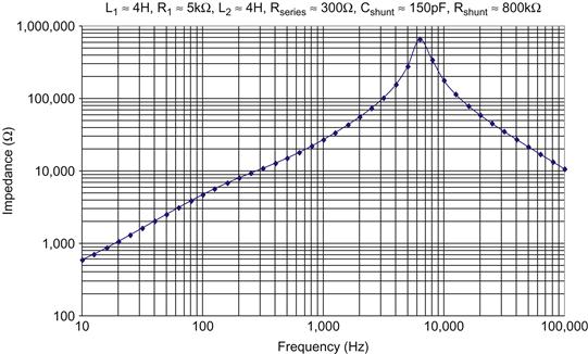
Figure A.2 If entered correctly, the impedance curve produced by the six-component model should look like this.
We can now play with model values. Presently, the circuit resonates at ≈6.3 kHz. Change Cshunt to 600 pF and it resonates at ≈3.15 kHz. Restore Cshunt to 150 pF. The circuit is quite undamped, and increasing Rshunt from 800k to 10,000k increases peak amplitude slightly, but reducing it to 10k flattens the curve. Restore Rshunt to 800k. Reduce L1 and L2 to 0.1 H, and note that the peak moves to 50 kHz. Reduce Rseries to 200 Ω, and note that the left-hand flat portion of the curve drops from 300 to 200 Ω (the new Rseries). Restore L1 and L2 to 4 H, but leave Rseries at 200 Ω. Toggle R1 between 5000 and 2000 Ω, and note that the kink in the rising curve below resonance moves from left to right (it’s harder to see this kink with only a few plotted points, but it’s there).
Having proven a theoretical model, we can now compare it to practical measurements. We type Vout in cell E1, set our function generator to its maximum sinusoidal output, measure VCycRMS using our digital oscilloscope, and enter that voltage, perhaps 5 V, in cell F1. We type rout in cell E2 and enter the function generator’s output resistance (probably 50 Ω) in cell F2.
We type Rseries in cell E3 and enter its value, perhaps 51 Ω, in cell F3 – we need to choose Rseries so that we never see more than Vout/2 in column B. 51 Ω is a minimum value, but we might need more. Be prepared to do a quick frequency sweep to estimate a suitable value – it isn’t critical. If you’re using this technique to measure from 10 Hz to 10 MHz, you might need to break the measurement into frequency bands and use different Rseries in different bands. Just add more cells below F3, label them, and refer to them at the appropriate frequencies.
We type Voltage in cell B8 and Impedance in cell C8. In cell C9 we type =($F$2+$F$3)/($F$1/B9-1) to calculate impedance from measured voltage, and we copy this cell down as necessary. We add a plot of column C against column A to our graph, and add the legend Measurement. We add the legend Model to our original curve.
We drive our test inductor from the function generator via Rseries, we invoke oscilloscope averaging over 32 traces, and use the oscilloscope’s automated measurements to measure VCycRMS directly across its terminals (thus making a four wire measurement), enter that value in cell B9, and its frequency in A9. We take as many measurements as necessary to give detail wherever we need it, then fit the model to the measurement. The “Sort” function in the “Data” menu becomes useful when extra measurements are added.
UK to US glossary
The author has been made aware that the UK and the US are two countries divided by a common language and that the innocent rugby term “hooker” has a different connotation in the US. In an effort to minimise the problem, the following non-inclusive glossary was kindly provided by Stuart Yaniger:
| UK | US |
| Allen key | hex wrench, Allen wrench |
| auto punch | generically referred to as center punch |
| bodging | improvising |
| dial gauge | runout gauge |
| dividers | compass |
| earth | ground |
| folding machine | sheet metal brake |
| G-clamp | C-clamp |
| Goddard’s Silver Dip | Tarn-X |
| haberdasher | specialist supplier of sewing materials |
| HT | high tension, high voltage, B+ |
| jigsaw | not the same as an American jigsaw – saber saw |
| knicker elastic | elastic band material, available at sewing supply shops |
| loft | attic |
| loo roll | toilet tissue |
| LT | low tension (invariably heater supply) |
| methylated spirits | denatured alcohol |
| mole wrench | vise grip |
| nutrunner | nut driver |
| Paxolin | Garolite |
| rugby | contact sport similar to American football, but without armour |
| semi-flush cutters | diagonal cutters |
| serrated/shakeproof washers | lockwashers |
| sheet metal punches | chassis punches |
| skip | dumpster |
| solder tags | solder lugs |
| spanner | wrench |
| tag strips | terminal strips |
| tension file | rod saw |
| tin snips | tin shears |
| valve | tube |
| washing-up liquid | detergent |