In Spark, the different linear methods use convex optimization to find the objective function. There are two types of optimization methods available in Spark—Stochastic Gradient Descent (SGD) and Limited memory Broyden Fletcher Goldfarb Shanno (L-BFGS)—of which SGD is more prominent in different algorithms. Which brings us to these different Linear algorithms—linear SVM, logistic regression, linear regression (using ordinary least squares, ridge regression, or Lasso). Note that there are variations of these algorithms with either SGD or L-BFGS. Spark also provides a streaming data variant of regression using the class StreamingLinearRegressionWithSGD. The following illustration shows how the linear regression algorithm forms a straight line:

The following illustration shows how the SVM algorithm finds the hyperplane that best separates points in a plane:

The Naive Bayes model is based on the Bayes rule, which finds the probability of a class label when we present it with the feature values of a data instance. When we derive this calculation using the Bayes rule, we will see that there are conditional dependencies among features, which are eliminated with a naive assumption; that probability of a class given a feature does not depend on any other feature value. This naive assumption defines the Naive Bayes model. This assumption also makes the Naive Bayes model a fast learning model and we can perform multiclass classification with high accuracy in practice.

Bayes rule:

The Bayes rule under naive assumption:

Decision trees are different to other models in the sense that they do not form a mathematical model for regression or classification. Rather, decision trees form an actual representation of yes/no decisions with a tree structure. We can perform both classification and regression using decision trees.

Spark also provides ensembles of decision trees—random forests and gradient boosted trees. An ensemble method is an approach to creating learning models where a model is composed of other similar models. In the case of a decision tree ensemble, majority voting is used to generate the final instance label.

Let's now see some examples of classification/regression algorithms in action. The first dataset we will consider is student grades datasets: https://archive.ics.uci.edu/ml/datasets/Student+Performance.

The student performance dataset can be termed as both a classification and a regression problem. Only one of 21 grades (0 to 20) is assigned to each student. Since the class label or the grade is discreet, countable and finite, we can use Naive Bayes multi-class classifier for this problem. We can also model this as regression problem by considering the target label as a real number.

First, let's take a look at the Naive Bayes implementation. Naive Bayes takes a lambda parameter with a value from 0 to 1. We try to vary this parameter in increasing order and then observe its effect on the predictions. Its code is as follows:

Here are the results, which show the effect of the lambda parameter on Root Mean Square Error (RMSE):

Next, we will implement a DecisionTree classifier as well as a DecisionTree regressor for the same problem and see how they perform on this problem.

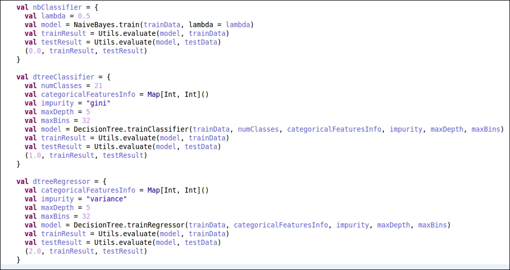
Here are the results of the three different algorithms:

As you can observe, the train accuracy for the regression tree is very low but that is because it is doing a one-to-one comparison. Since the regression tree will generate a real valued output, it is likely that the label will be a mismatch by a very small value but will still fail the equals comparison. However, when we look at the RMSE for both train and test data, we observe a significant decrease in the overall error. So for this dataset, it seems like regression is the correct algorithm to choose. Also, we should notice that the grades have a default ordering, that is a grade with higher value means a bigger grade. However, for problems where there is no implicit ordering among different class labels, we should go for a classification algorithm.

The next dataset that we will explore is TV News Channel Commercial Detection Dataset Data Set from here: https://archive.ics.uci.edu/ml/datasets/TV+News+Channel+Commercial+Detection+Dataset.

Let's download the dataset into the datasets folder inside the codebase using the following commands:

$ cd code/datasets/
$ wget -c https://archive.ics.uci.edu/ml/machine-learning-databases/00326/TV_News_Channel_Commercial_Detection_Dataset.zip
$ mkdir TVData/
$ cd TVData/
$ unzip ../TV_News_Channel_Commercial_Detection_Dataset.zip

This dataset is available to us in the LibSVM format so it is fairly easy to load into Spark. We have data for five news channels—CNN IBN, NDTV 24X7, Times Now, BBC, and CNN. The data for each of the channels is present in a separate text file, so in total we have five text files (LibSVM format). We don't need to do any processing except to concatenate them. The class labels are binary so we can use any binary classification algorithm: SVM, Naive Bayes, logistic regression, and so on. The total dataset size is 191 MB uncompressed.

For this problem, we will first use the Naive Bayes binary classifier. The code is exactly the same as the one we used for the student performance dataset.

Its code is as follows:

$ cd code/
$ sbt "run-main chapter04.TVNewsChannelsNaiveBayes datasets/TVData/"
... OUTPUT SKIPPED ...
$ python scripts/ch04/student-grade-plots.py

Here are the results with varying lambda values:

The change in error is not significant. The train error drops in the range 0.4 to 0.9 and then rises again from 0.9 to 1.0. The test error consistently drops for values of lambda from 0.1 to 0.4 and then increases. So, if we were to choose a lambda value, we could choose it somewhere near 0.4.

Now let's look at how this problem behaves when using a decision tree regression algorithm.

Its code is as follows:

$ cd code/
$ sbt "run-main chapter04.TVNewsChannelComparison datasets/TVData/"
... OUTPUT SKIPPED …
$ python scripts/ch04/tv-news-plots.py

This code was run on a single machine so it took some time. We can also take a look at the progress using Spark UI:

Here are the final results:

As we observed with the student dataset, the train/test accuracy is very low (the reason was also mentioned earlier). Again, we can see a significant increase in the RMSE values.