APPENDICES

Background and Prerequisite for Predictive Analytics

APPENDIX A: Probability Concepts: Role of Probability and Probability Distributions in Decision Making

APPENDIX B: Sampling, Sampling Distribution, and Inference Procedure

APPENDIX C: Review of Estimation, Confidence Intervals, and Hypothesis Testing

APPENDIX D: Hypothesis Testing for One and Two Population Parameters

APPENDIX A

Probability Concepts: Role of Probability in Decision Making

Review of Probability: Theory and Formulas

Some important terms of probability theory.

Event: An event is one or more possible outcomes of an experiment.

Experiment: An experiment is any process that produces an outcome or observation. For example, throwing a die is a simple experiment and getting a number (1 or 2…, or 6) on the top face is an event. Similarly, tossing a coin is an experiment and getting a head (H) or a tail (T) is an event.

In probability theory, we use the term experiment in a very broad sense. We are interested in an experiment whose outcome cannot be predicted in advance.

Sample Space: The set of all possible outcomes of an experiment is called the sample space and is denoted by the letter S.

The probability of an event A is denoted as P(A), which means the “probability that event A occurs.” That probability is between 0 and 1. In other words,

Mutually Exclusive Events: When the occurrence of one event excludes the possibility of the occurrence of another event, the events are mutually exclusive. In other words, one and only one event can take place at a time.

Exhaustive Events: The total number of possible outcomes in any trial is known as exhaustive events. For example, in a roll of two dice, the exhaustive number of events or the total number of outcomes is 36. If three coins are tossed at the same time, the total number of outcomes is 8 (try to list these outcomes).

Equally Likely Events: All the events have an equal chance of occurrence or there is no reason to expect one in preference to the other.

Counting Rules in Probability

1. 1.Multiple-Step Experiment or Filling Slots

Suppose an experiment can be described as a sequence of k steps in which

n₁ = the number of possible outcomes in the first step

n₂ = the number of possible outcomes in the second step

⋮

n_k = the number of possible outcomes in the kth step,

then the total number of possible outcomes is given by

1. 2.Permutations

The number of ways of selecting n distinct objects from a group of N objects—where the order of selection is important—is known as the number of permutations on N objects using n at a time and is written as

1. 3.Combinations

Combination is selecting n objects from a total of N objects. The order of selection is not important in combination. This disregard of arrangement makes the combination different from the permutation. In general, an experiment will have more permutations than combinations.

The number of combinations of N objects taken n at a time is given by

Assigning Probabilities

There are two basic rules for probability assignment.

1. 1.The probability of an event A is written as P(A) and it must be between 0 and 1. That is,

   

2. 2.If an experiment results in n number of outcomes A₁, A₂..., A_n, then the sum of the probabilities for all the experimental outcomes must equal 1. That is,

Methods of Assigning Probabilities

There are three methods for assigning probabilities

1. 1.Classical Method
2. 2.Relative Frequency Approach
3. 3.Subjective Approach

1. 1.Classical Method

The classical approach of probability is defined as the favorable number of outcomes divided by the total number of possible outcomes. Suppose an experiment has n number of possible outcomes and the event A occurs in m of the n outcomes, then the probability that event A will occur is

Note that P(A) denotes the probability of occurrence for event A. The probability that event A will not occur is given by P(Ā), which is read as P (not A) or “A complement.” Thus,

which means that the probability that event A will occur plus the probability that event A will not occur must be equal to 1.

1. 2.Relative Frequency Approach

Probabilities are also calculated using relative frequency. In many problems, we define probability by relative frequency.

1. 3.Subjective Probability

Subjective probability is used when the events occur only once or very few times and when little or no relevant data are available. In assigning subjective probability, we may use any information available, such as our experience, intuition, or expert opinion. In this case the experimental outcomes may not be clear and relative frequency of occurrence may not be available. Subjective probability is a measure of our belief that a particular event will occur. This belief is based on any information that is available to determine the probability.

Addition Law for Mutually Exclusive Events

If we have two events A and B that are mutually exclusive, then the probability that A or B will occur is given by

Note that the “union” sign is used for “or” probability, that is, P(A∪B). This is the same as P (A or B). This rule can be extended to three or more mutually exclusive events. If three events A, B, and C are mutually exclusive, then the probability that A or B or C will happen can be given by

Addition Law for Non-Mutually Exclusive Events

The occurrence of two events that are non-mutually exclusive means that they can occur together. If the events A and B are non-mutually exclusive, the probability that A or B will occur is given by

If events A, B, and C are non-mutually exclusive, then the probability that A or B or C will occur is given by

or

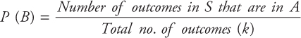
Probabilities of Equally Likely Events

Equally Likely Events are those that have an equal chance of occurrence or those where there is no reason to expect one in preference to the other. In many experiments it is natural to assume that each outcome in the sample space is equally likely. Suppose that the sample space S consists of k outcomes, where each outcome is equally likely to occur. The k outcomes of the sample space can be denoted by S = {1,2,3,...,k} and

P(1) = P(2) = ... = P(k)

That is, each outcome has an equal probability of occurrence.

The above implies that the probability of any event B is

Probabilities under Conditions of Statistical Independence

When two or more events occur, the occurrence of one event has no effect on the probability of occurrence of any other event. In this case, the events are considered independent. There are three types of probabilities under statistical independence:

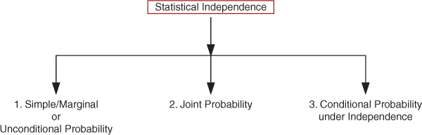
1. 1.Simple probability is also known as marginal or unconditional and is the probability of occurrence of a single event, say A, and is denoted by P (A).

P(A) = marginal probability of event A

P(B) = marginal probability of event B

1. 2.Joint Probability under Statistical Independence

Joint probability is the probability of occurrence of two or more events together or in succession. It is also known as “and” probability. Suppose we have two events, A and B, which are independent. Then the joint probability, P(AB), which is the probability of occurrence of both A “and” B, is given by

The probability of two independent events occurring together or in succession is the product of their marginal or simple probabilities.

Note that P(AB) = probability of event A and B occurring together, which is known as joint probability. P(AB) is the same as P(A and B) or P(A∩B).

Events A and B are independent and can be extended to more than two events. For example,

is the probability of three independent events, A, B, and C, which is calculated by taking the product of their marginal or simple probabilities.

1. 3.Conditional Probability under Statistical Independence

The conditional probability is written as

and is read as the probability of event A, given that B has occurred, or the probability of A, given B. If the two events A and B are independent, then

This means that if the events are independent, the probabilities are not affected by the occurrence of each other. The probability of occurrence of B has no effect on the occurrence of A. That is, the condition has no meaning if the events are independent.

Statistical dependence

When two or more events occur, the occurrence of one event has an effect on the probability of the occurrence of any other event. In this case, the events are considered to be dependent.

There are three types of probabilities under statistical dependence.

1. 1.Conditional Probability under Statistical Dependence

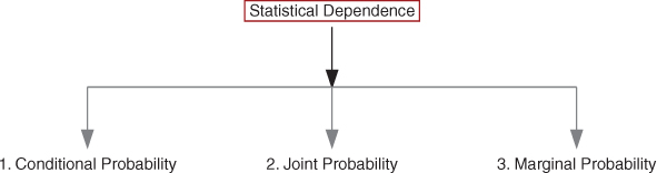
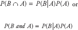
1. 2.Joint Probability under Statistical Dependence

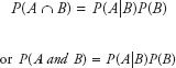
Similarly,

1. 3.Marginal Probability under Statistical Dependence

The marginal probability under statistical dependence is explained using the joint probability table below.

	Dotted (D)	Striped (S)	Total
Red (R)	0.30	0.10	0.40
Green (G)	0.20	0.40	0.60
Total	0.50	0.50	1.00

From the above table,

Bayes’ Theorem

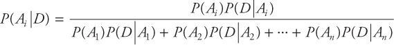
The above equation can be used to compute any posterior probability P(A_i|D) when prior probabilities P(A₁),P(A₂),...,P(A_n) and conditional probabilities P(D|A₁),P(D|A₂),...,P(D|A_n) are known.

Role of Probability Distributions in Decision Making

Probability Distributions

The graphical and numerical techniques discussed and used in descriptive analytics (the first volume of this book) are very helpful in getting insight and describing the sample data. These methods help us draw conclusions about the process from which data are collected.

In this section, we will study several of the discrete and continuous probability distributions and their properties, which are a critical part of data analysis and predictive modeling. A good knowledge and understanding of probability distributions helps an analyst to apply these distributions in data analysis. The probability distributions are an essential part of decision-making process. The application of key predictive analytics models including all types of regression, nonlinear regression and modeling, forecasting, data mining, and computer simulation all use probability and probability distributions.

Here we discuss some of the important probability distributions that are used in analyzing and assessing the regression and predictive models. The knowledge and understanding of two important distributions—the normal and t-distributions—are critical in analyzing and checking the adequacy of the regression models. Before we discuss these distributions in detail, we will provide some background information about the distributions.

Probability Distribution and Random Variables

The probability distribution is a model that relates the value of a random variable with the probability of occurrence of that value.

A random variable is a numerical value that is unknown and may result from a random experiment. The numerical value is a variable and the value achieved is subject to chance and is, therefore, determined randomly. Thus, a random variable is a numerical quantity whose value is determined by chance. Note that a random variable must be a numerical quantity.

Types of random variable: Two basic types of random variables are discrete and continuous variables, which can be described by discrete and continuous probability distributions.

Discrete Random Variable

A random variable that can assume only integer value or whole number is known as discrete. An example would be the number of customers arriving at a bank. Another example of a discrete random variable would be rolling two dice and observing the sum of the numbers on the top faces. In this case, the results are 2 through 12. Also, note that each outcome is a whole number or a discrete quantity. The random variable can be described by a discrete probability distribution.

Table A.1 shows the discrete probability distribution (in a table form) of rolling two dice and observing the sum of the numbers. In rolling two dice and observing the sum of the numbers on the top faces, the outcome is denoted by x which is the random variable that denotes the sum of the numbers.

Table A.1

The outcome X (which is the sum of the numbers on the top faces) takes on different values each time the pair of dice is rolled. On each trial, the sum of the numbers is going to be a number between 2 and 12 but we cannot predict the sum with certainty in advance. In other words, the outcomes or the occurrence of these numbers is a chance factor. The probability distribution is the outcomes X_i, and the probabilities for these outcomes P(X_i). The probability of each outcome of this experiment can be found by listing the sample space of all 36 outcomes. These can be shown both in a tabular and in a graphical form. Figure A.1 shows the probability distribution graphically. The following are the two requirements for the probability distribution of a discrete random variable:

1. 1.P(x) is between 0 and 1 (both inclusive) for each x, and
2. 2.

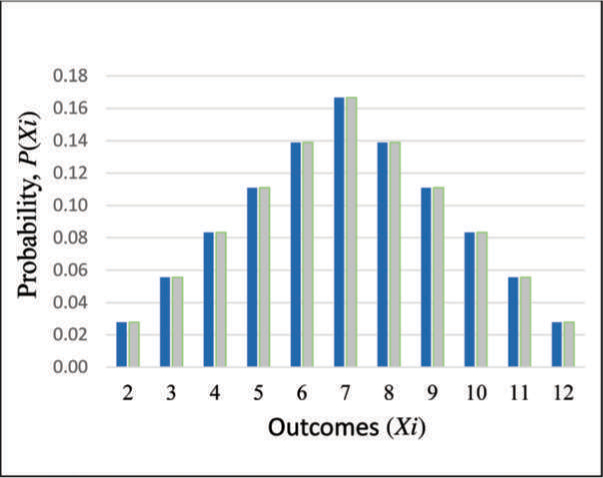
Figure A.1: Probability Distribution of Rolling Two Dice

In summary, the relationship between the values of a random variable and their probabilities is summarized by a probability distribution. A probability distribution of a random variable is described by the set of possible random variables’ values and their probabilities. The probability distribution provides the probability for each possible value or outcome of a random variable. A probability distribution may also be viewed as the shape of the distribution. The foundation of probability distributions is the laws of probability. Note that most of the phenomenon in real-world situation is random in nature. In a production situation, finding the number of defective product might be seen as a random variable because it takes on different values according to some random mechanism.

Expected Value, Variance, and Standard Deviation of a Discrete Distribution

The mean or the expected value of a discrete random variable denoted by μ, or E(x) is the average value observed over a long period. The variance and standard deviation σ² and σ, respectively, are the measures of variation of the random variable.

In this section, we will demonstrate how to calculate the expected value, variance, and standard deviation for a discrete probability distribution. We will use the concept of the mean or expected value and variance in the next section.

Background: The mean for a discrete random variable is defined mathematically as the expected value and is written as:

The variance of a discrete random variable is defined as:

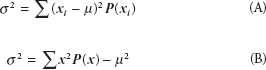
The standard deviation,

Example A.1

Table A.2 shows the number of cars sold over the past 500 days for a particular car dealership in a certain city.

Table A.2: Number of Cars Sold

(1) No. of Cars Sold (xi)	(2) Frequency (fi)	(3) Relative Frequency, P(xi)
0	40	40/500 = 0.08
1	100	0.200
2	142	0.284
3	66	0.132
4	36	0.072
5	30	0.060
6	26	0.052
7	20	0.040
8	16	0.032
9	14	0.028
10	8	0.016
11	2	0.004
Total	500	1.00

[a] Calculate the relative frequency

The relative frequencies are shown in column (3) of Table A.2. Note that the relative frequency distribution is calculated by dividing the frequency of the class by the total frequency, which is also the probability, P(x).

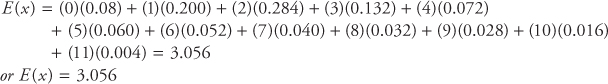
[b] Calculate the expected value or the mean number of cars sold

The expected value is given by:

or

[c] Calculate the variance and the standard deviation

The variance for this discrete distribution is given by

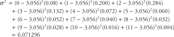
The variance can be more easily calculated using equation (2.5) with (B). The standard deviation for this discrete distribution is

[d] Find the probability of selling less than four cars

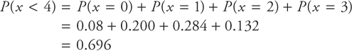
These probability values are obtained from Table A.2 column (3).

[e] Find the probability of selling at most four cars

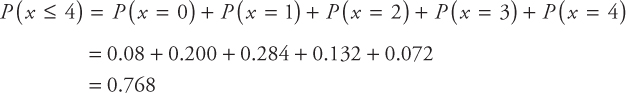
[f] What is the probability of selling at least four cars?

The above probability can also be calculated as

Continuous Random Variables

The random variable that might assume any value over a continuous range of possibilities is known as continuous random variables. Some examples of continuous variables are physical measurements of length, volume, temperature, or time. These variables can be described using continuous distributions.

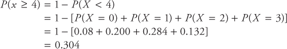
The continuous probability distribution is usually described using a probability density function. The probability density function, f(x), describes the behavior of a random variable. It may be viewed as the shape of the data. Figure A.2 shows the histogram of the diameter of a machined parts with a fitted curve. It is clear that the diameter can be approximated by certain patterns that can be described by a probability distribution.

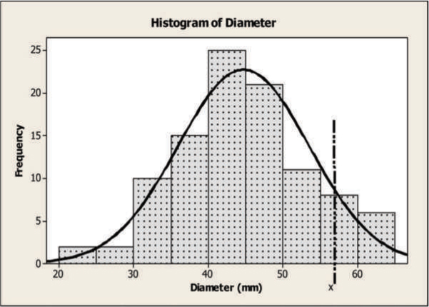
Figure A.2: Diameter of Machined Parts

The shape of the curve in Figure A.2 can be described by a mathematical function, f(x), or a probability density function. The area below the probability density function to the left of a given value, x, is equal to the probability of the random variable (the diameter in this case) shown on the x-axis. The probability density function represents the entire sample space; therefore, the area under the probability density function must equal one.

The probability density function, f(x), must be positive for all values of x (as negative probabilities are impossible). Stating these two requirements mathematically,

and f(x) > 0 for continuous distributions. For discrete distributions, the two conditions can be written as

To demonstrate how the probability density function is used to compute probabilities, consider Figure A.3. The shape in the figure can be well approximated by a normal distribution. Assuming a normal distribution, we would like to find the probability of a diameter below 40 mm. The area of the shaded region represents the probability of a diameter, drawn randomly from the population having a diameter less than 40 mm. This probability is 0.307 or 30.7 percent using a normal probability density function. Figure A.4 shows the probability of the diameter of one randomly selected machined part having a diameter ≥ 50 mm but ≤ 55 mm. Here we discuss some of the important continuous and discrete distributions.

Figure A.3: An Example of Calculating Probability using Probability Density

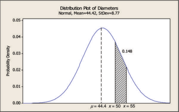
Figure A.4: Another Example of Calculating Probability Using Probability Density

Some Important Continuous Distributions

In this section we will discuss the continuous probability distributions. When the values of random variables are not countable but involve continuous measurement, the variables are known as continuous random variables. Continuous random variables can assume any value over a specified range. Some examples of continuous random variables are:

• •The length of time to assemble an electronic appliance
• •The life span of a satellite power source
• •Fuel consumption in miles-per-gallon of new model of a car
• •The inside diameter of a manufactured cylinder
• •The amount of beverage in a 16-ounce can
• •The waiting time of patients at an outpatient clinic

In all the above cases, each phenomenon can be described by a random variable. The variable could be any value within a certain range and is not a discrete whole number. The graph of a continuous random variable x is a smooth curve. This curve is a function of x, denoted by f(x), and is commonly known as a probability density function. The probability density function is a mathematical expression that defines the distribution of the values of the continuous random variable. Figure A.5 shows examples of three continuous distributions.

One of the most widely used and important distributions of our interest is the Normal Distribution. The other distributions of importance are the t-distribution and F-distribution. We discuss all of these here.

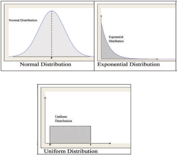
Figure A.5: Examples of Three Continuous Distributions

The Normal Distribution

Background: A continuous random variable X is said to follow a normal distribution with parameters µ and σ and the probability density function of X is given by:

where f (x) is the probability density function, µ the mean, σ the standard deviation, and e = 2.71828, which denotes the base of the natural logarithm. The distribution has the following properties:

1. The normal curve is a bell-shaped curve. It is symmetrical about the line x = µ. The mean, median, and mode of the distribution have the same value.

2. The parameters of normal distribution are the mean µ and standard deviation σ. The interpretation of how the mean and standard deviation are related in a normal curve is shown in Figure A.6.

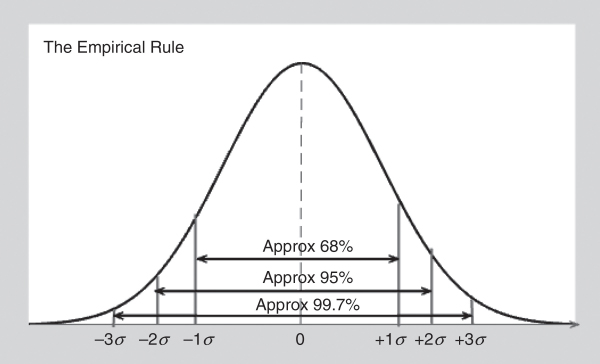
Figure A.6: Areas under the Normal Curve

Figure A.6 states the area property of the normal curve. For a normal curve, approximately 68 percent of the observations lie between the mean and ±1σ (one standard deviation), approximately 95 percent of all observations lie between the mean and ±2σ (two standard deviations), and approximately 99.73 percent of all observations fall between the mean and ±3σ (three standard deviations). This is also known as the empirical rule.

The shape of the curve depends on the mean (µ) and standard deviation (σ). The mean µ determines the location of the distribution, whereas the standard deviation σ determines the spread of the distribution. Note that larger the standard deviation (σ), more spread out is the curve (see Figure A.7).

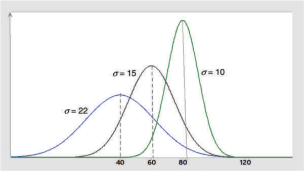
Figure A.7: Normal Curve with Different Values of Mean and Standard Deviation

The Standard Normal Distribution

To calculate the normal probability, where X is a normal variate with parameters µ and σ, we need to evaluate:

To evaluate the above expression in (A), none of the standard integration techniques can be used. However, the expression can be numerically evaluated for µ = 0 and σ = 1. When the values of the mean µ and standard deviation σ are 0 and 1, respectively, the normal distribution is known as the standard normal distribution.

The normal distribution with µ = 0 and σ = 1 is called a standard normal distribution. Also, a random variable with standard normal distribution is called a standard normal random variable and is usually denoted by Z.

The probability density function of Z is given by

The cumulative distribution function of Z is given by:

which is usually denoted by Φ (z).

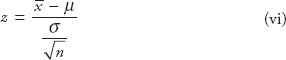
When the random variable X is normally distributed with mean µ and variance σ², that is, x : N(µ, σ²), we can calculate the probabilities involving x by standardizing. The standardized value is known as the standard or standardized normal distribution and is given using expression (B):

As indicated above, if x is normally distributed with mean µ and standard deviation σ, then

is a standard normal random variable where,

z = distance from the mean to the point of interest (x) in terms of standard deviation units

x = point of interest

µ = the mean of the distribution, and

σ = the standard deviation of the distribution.

Finding Normal Probability by Calculating Z-Values and using the Standard Normal Table

Equation (B) above is a simple equation that can be used to evaluate the probabilities involving normal distribution.

Example A.2

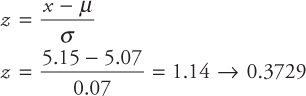
The inside diameter of a piston ring is normally distributed with a mean of 5.07 cm and a standard deviation of 0.07 cm. What is the probability of obtaining a diameter exceeding 5.15 cm?

The required probability is the shaded area shown in Figure A.8. To determine the shaded area, we first find the area between 5.07 and 5.15 using the z-score formula and then subtract the area from 0.5. See the calculations below.

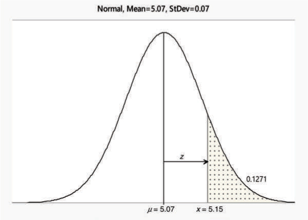
Figure A.8: Area Exceeding 5.15

Note: 0.3729 is the area corresponding to z = 1.14. This can be read from the table of Normal Distribution provided in the Appendix. There are many variations of this table. The normal table used here provides the probabilities on the right side of the mean.

The required probability is

or, there is 12.71 percent chance that piston ring diameter will exceed 5.15 cm.

Example A.3

The measurements on certain types of PVC pipes are normally distributed with a mean of 5.01 cm and a standard deviation of 0.03 cm. The specification limits on the pipes are 5.0±0.05 cm. What percentage of the pipes is not acceptable?

The percentage of acceptable pipes is the shaded area shown in Figure A.9. The required area or the percentage of acceptable pipes is explained below.

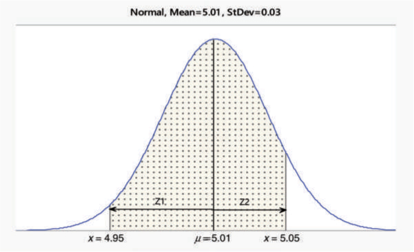
Figure A.9: Percent Acceptable (Shaded Area)

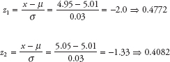
The area 0.4772 is the area between the mean 5.01 and 4.95 (see Figure A.9). The area left of 4.95 is 0.5 – 0.4772 = 0.0228.

The area 0.4082 is the area between the mean 5.01 and 5.05. The area right of 5.05 is 0.5 – 0.4082 = 0.0918.

Therefore, the percentage of pipes not acceptable = 0.0228 + 0.0918 = 0.1146 or 11.46 percent. These probabilities can also be calculated using a statistical software.

Probability Plots

Probability plots are used to determine if a particular distribution fits sample data. The plot allows us to determine whether a distribution is appropriate and also to estimate the parameters of fitted distribution. The probability plots are a good way of determining whether the given data follow a normal or any other assumed distribution. In regression analysis, this plot is of great value because of its usefulness in verifying one of the major assumption of regressions—the normality assumption.

MINITAB and other statistical software provide options for creating individual probability plots for the selected distribution for one or more variables. The steps to probability plotting procedure are:

1. 1.Hypothesize the distribution: select the assumed distribution that is likely to fit the data
2. 2.Order the observed data from smallest to largest. Call the observed data x₁, x₂, x₃,....., x_n
3. 3.Calculate the cumulative percentage points or the plotting position (PP) for the sample of size n (i = 1,2,3,...,n) using the following:

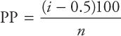
1. 4.Tabulate the x_i values and the cumulative percentage (probability values or PP). Depending on the distribution and the layout of the paper, several variations of cumulative scale are used.
2. 5.Plot the data using the graph paper for the selected distribution. Draw the best fitting line through these points.
3. 6.Draw your conclusion about the distribution.

MINITAB provides the plot based on the above steps. To test the hypothesis, an Anderson-Darling (AD) goodness-of-fit statistic and associated p-value can be used. These values are calculated and displayed on the plot. If the assumed distribution fits the data:

• •the plotted points will form a straight line (or approximate a straight line)
• •the plotted points will be close to the straight line
• •the Anderson-Darling (AD) statistic will be small, and the p-value will be larger than the selected significance level, α (commonly used values are 0.05 and 0.10).

Example A.4 Probability Plot (1)

To demonstrate the probability plot, consider the length of measurements of 15 PVC pipes from a manufacturing process. We want to use the probability plot to check whether the data follow a normal distribution. The probability plot is shown in Figure A.10. From the plot we can see that the cumulative percentage points approximately form a straight line and the points are close to the straight line. The calculated p-value is 0.508. At a 5 percent level of significance (α = 0.05), p-value is greater than α so we cannot reject the null hypothesis that the data follow a normal distribution. We conclude that the data follow a normal distribution.

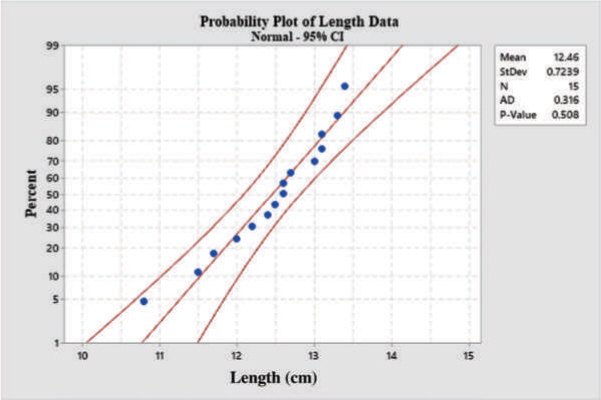
Figure A.10: Probability Plot of Length Data

Example A.5 Probability Plot (2)

A probability plot can be used in place of a histogram to determine the process capability and can also be used to determine the distribution and shape of the data. If the probability plot indicates that the distribution is normal, the mean and standard deviation can be estimated from the plot. Figure A.11 shows the histogram and probability plot for the length measurements and failure time data. As can be noted, the histogram of the length data is clearly normally distributed, whereas the histogram of the failure time is not symmetrical and might follow an exponential distribution. The probability plots of both the length and the failure time are plotted next to the histograms.

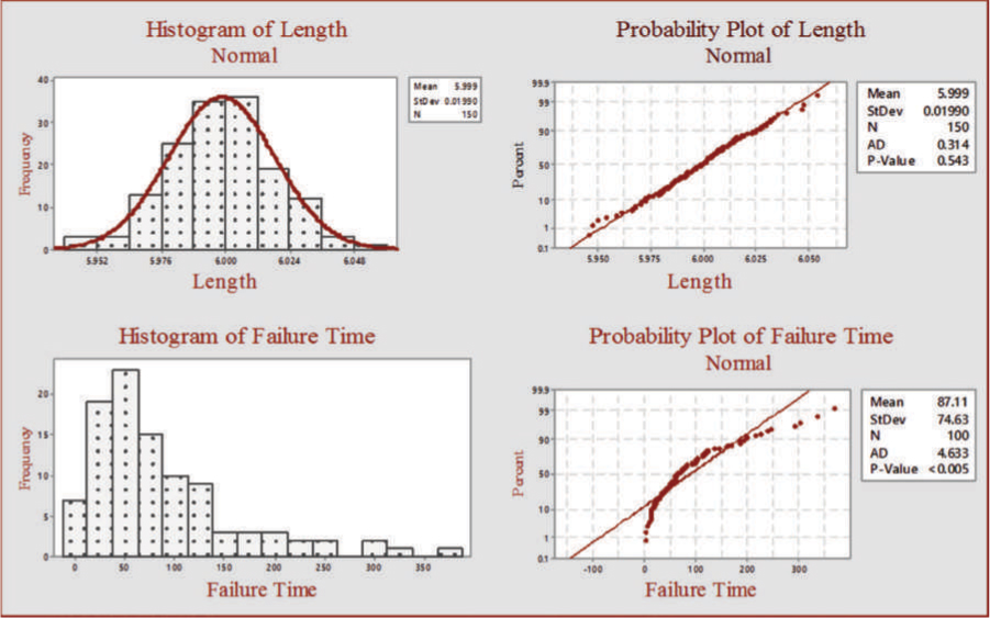
Figure A.11: Histograms and Probability Plots of Length and Failure Time Data

From the probability plot of the length data (Figure A.11), we can see that the cumulative percentage points approximately form a straight line and the points are close to the straight line. The calculated p-value is 0.543. At a 5 percent level of significance (α = 0.05), p-value is greater than α so we cannot reject the null hypothesis that the data follow a normal distribution. We conclude that the data follow a normal distribution. The probability plot of failure time data shows that the cumulative percentage points do not form a straight line. The plotted points show a curvilinear pattern. The calculated p-value is less than 0.005. At a 5 percent level of significance (α = 0.05), p-value is less than α so we reject the null hypothesis that the data follow a normal distribution. The deviation of the plotted points from a straight line is an indication that the failure time data do not follow a normal distribution. This is also evident from the histogram of the failure data.

Checking whether the Data Follow a Normal Distribution: Assessing Normality

Statistics and data analysis cases involve making inferences about the population based on the sample data. Several of these inference procedures are discussed in the chapters that follow. Many of these inference procedures are based on the assumption of normality; that is, the population from which the sample is taken follows a normal distribution. Before we draw conclusions based on the assumption of normality, it is important to determine whether the sample data come from a population that is normally distributed. Below we present several descriptive methods that can be used to check whether the data follow a normal distribution. Methods most commonly used to assess the normality are described in Table A.3.

Table A.3: Checking for Normal Data

1.Construct a histogram or stem-and-leaf of the data. The shape of the histogram and stem-and-leaf plots will resemble a normal curve if the data are normal or approximately normal. 2.Calculate the mean, median, and mode (if appropriate) of the data. If these measures are approximately equal, then the data are symmetrical or approximately normal. 3.Calculate the mean and standard deviation and the intervals and If the data are normal, the observations for these intervals would be approximately 68%, 95%, and 99.7%, respectively. 4.Construct a box plot of the data using the five-measure summary: minimum, Q1, Q2, Q3, and the maximum. If the data are normal, the distance from minimum data value to Q1 and Q3 to maximum data value will be approximately equal. In addition, the median (Q2) will divide the box into approximately two equal halves. 5.Calculate the interquartile range (IQR) and the standard deviation, s, of the sample data. If the ratio IQR / s = 1.3 then the data are normal or approximately normal. 6.Construct a normal probability plot of the data. If the data are normal or approximately normal, the points on the probability plot will fall on a straight line.

Example A.6: Checking for Normal Data

A consultant hired by a hospital management to study the waiting time of patients at the hospital emergency service collected the data shown in Table A.4. The table shows the waiting time (in minutes) for 150 customers.

Table A.4: Waiting Time (in minutes)

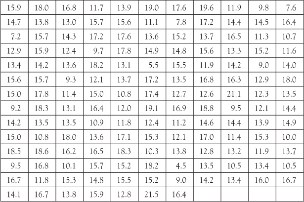
The distribution of the waiting time data is of interest to draw certain conclusions. To check whether the waiting time data follow a normal distribution, numerical and graphical analyses were conducted. The analysis methods outlined in Table A.3 were performed on the data. The results are shown below.

Graphical and numerical analyses: Figure A.12 shows the histogram with the normal curve, a box plot of the data along with descriptive statistics calculated from the data.

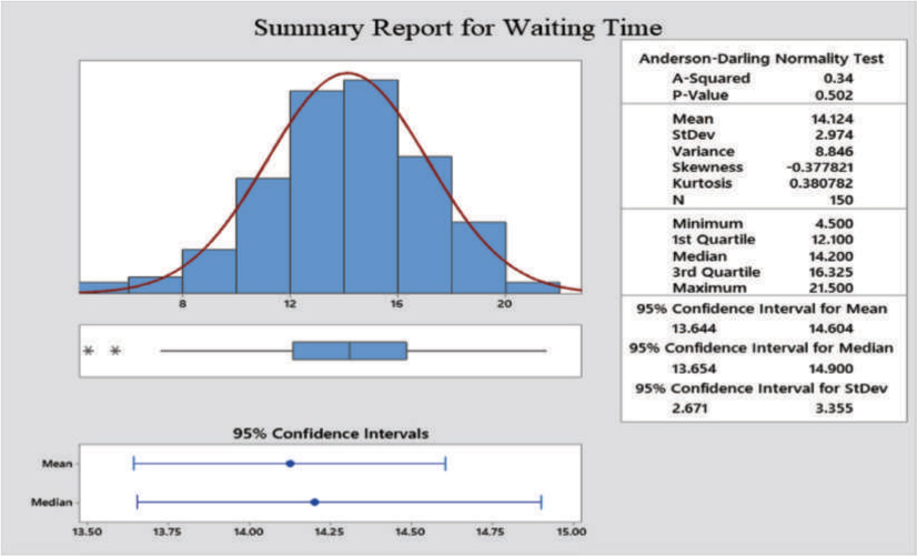
Figure A.12: Graphical and Numerical Summary of Waiting Time

Check #1

The histogram of the data in Figure A.12 indicates that the shape very closely resembles a bell shape or normal distribution. The bell curve superimposed over the histogram shows that the data have a symmetric or normal distribution centered around the mean. Thus, we can conclude that the data follow a normal distribution.

Check #2

The values of mean and the median in Figure A.12 are 14.124 and 14.200, respectively. If the data are symmetrical or normal, the values of the mean and median are very close. Since the mean and median for the waiting time data are very close, it indicates that the distribution is symmetrical or normal.

Check #3

Check #3 requires that we calculate the percentages of the observations falling between the mean and one, two, and three standard deviations. If the data are symmetrical or normal, approximately 68 percent of all observations will fall between the mean and ±one standard deviation, approximately 95 percent all observations will fall between the mean and ±two standard deviations, and approximately 99.7 percent of all observations will fall between the mean and ±three standard deviations. For the waiting time data the mean and standard deviation Table A.5 shows the percentages for the waiting time data between the mean and ±one, two, and three standard deviations.

Table A.5: Percentages between One, Two, and Three Standard Deviations

Interval	Percentage in Interval
	69.3
	95.3
	99.3

The percentages between the mean and standard deviation of the example problem (Table A.4 data) agree with the empirical rule or the normal distribution.

Check #4

The box plot of the data in Figure A.12 shows that the waiting time data very closely follow a normal distribution.

Check #5

The ratio of the IQR to the standard deviation is calculated below. The values are obtained from Figure A.12.

The value is close to 1.3, indicating that the data are approximately normal.

Check #6

This check involves constructing a normal probability plot of the data. This plot is shown in Figure A.13. In a probability plot, the ranked data values are plotted on the x-axis and their corresponding z-scores from a standard normal distribution are plotted on the y-axis. If the data are normal or approximately normal, the points will plot on an approximate straight line. The normal probability plot of waiting time data shows that the data are very close to a normal distribution.

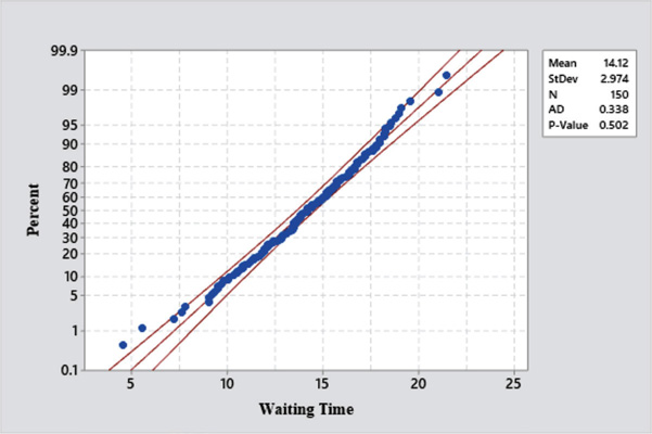
Figure A.13: Probability Plot of Waiting Time

All of the above checks confirm that the waiting time data very closely follow a normal distribution.

Student t-Distribution

This is one of the useful sampling distributions related to the normal distribution. This distribution is used to check the adequacy of the regression models. Suppose x is a normally distributed random variable with mean 0 and variance 1. Suppose we have another random variable χ_n² with n degrees of freedom, then the random variable t_n is given by:

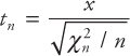
which follows a t-distribution with (n - 1) degrees of freedom. Like the normal distribution, this distribution is also symmetrical about the mean, µ = 0, and its range extends from –∞ < x < ∞. As the degrees of freedom increase, the t-distribution approaches the normal distribution.

As an example of a random variable that is t-distributed, consider the sampling of the sample mean. We have seen that the normal distribution is based on the assumption that the mean µ and the standard deviation σ of the population are known. In calculating the normal probabilities using the formula z = (x – µ)/σ the statistic z is calculated on the basis of a known σ. However, in most cases σ is not known and is estimated using the sample standard deviation s whose distribution is not normal when the sample size n is small (<30).

In sampling from a population that is normally distributed, the fraction follows a normal distribution, but if σ is not known and n is small, will not be normally distributed. It was shown by Gosset that the random variable follows the distribution known as the t-distribution. The statistic t has a mean = 0 and a variance >1 (unlike the standard normal distribution whose mean = 0 and variance = 1). Since the variance is greater than 1, this distribution is less peaked at the center compared to the normal distribution and is also higher in the tails compared to the normal distribution. As the sample size n becomes larger, the t-distribution comes closer and closer to the normal distribution. In the next section, we have performed an experiment to gain further insight into the t-distribution.

Comparing the Normal and t-Distribution

Objective: Compare the shapes of the normal distribution and the t-distribution and show that as the degrees of freedom for the t-distribution increase (or the sample size n increases), the t-distribution will approach a normal distribution. We will also see that the t-distribution is less peaked at the center and higher in the tails than the normal distribution.

Problem Statement: In this experiment, we will graph the normal probabilities with mean µ = 0 and standard deviation σ = 1 and compare it to the probability density functions of t-distribution with 1, 3, 5, and 10 degrees of freedom. We will plot the normal and t-distributions on the same plot and compare the shapes of the t-distributions for different degrees of freedom to that of the normal distribution. The steps are outlined below.

• •Using MINITAB, calculate the normal probability densities for x = –4 to 4 with mean µ = 0 and standard deviation σ = 1.0.
• •Calculate the probability density function for the t-distribution with 1, 3, 5, and 10 degrees of freedom for the same values of x as above and store your results.
• •Graph the normal density function and the density functions for the t-distribution for 1, 3, 5, and 10 degrees of freedom on one plot. This will help us compare the shape of the normal distribution and various t-distributions. The plot will be similar to the one shown in Figure A.14.

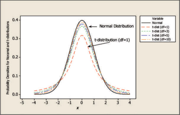
Figure A.14: Comparison between Normal and t-Distributions (df = degrees of freedom)

From Figure A.14, the innermost curve is the probability density for t-distribution with one degree of freedom and the outermost curve is the density function of a normal distribution. You can see that as we increase the number of degrees of freedom for the t-distribution, the shape approaches a normal distribution. Also, note that the t-distribution is less peaked at the center and higher in the tails compared to the normal distribution.

F-distribution

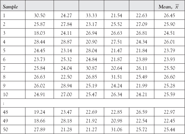
The F-distribution discussed in this section is also related to the normal distribution. To get an understanding of the F-distribution, suppose that χ_u² and χ_v² are two independent χ² random variables with u and v degrees of freedom, respectively, then the ratio

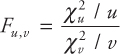
follows an F distribution with u as the numerator degrees of freedom and v as the denominator degrees of freedom. The range of values of F is from 0 to +∞ since the values of χ_u² and χ_v² are all non-negative. As an application of this distribution, consider the following example where we sample from the F-distribution.

Suppose we have two independent normal variables x₁ and x₂ with the following mean and variances and and we draw samples of size n₁ and n₂ from the first and second normal process. If the sample variances are s₁² and s₂², then the ratio

follows an F-distribution with (n₁−1) and (n₂−1) degrees of freedom. The shape of the F-distribution depends on the numerator and denominator degrees of freedom. As the degrees of freedom increase, the distribution approaches the normal distribution. In Figure A.15 we have graphed several F-distributions with different degrees of freedom.

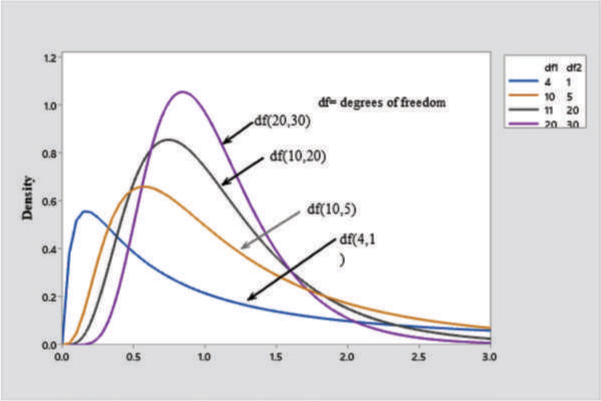
Figure A.15: F-Distribution for Various Degrees of Freedom

F-distribution is the appropriate distribution for comparing the ratio of two variances. In regression analysis, the distribution is used in conducting the F-test to check for the overall significance of the regression model.

Summary

In this section, we provided an overview of statistical methods used in analytics. A number of statistical techniques both graphical and numerical were presented. These descriptive statistical tools are used in modeling, studying, and solving various problems. The graphical and numerical tools of descriptive statistics are also used to describe variation in the process data. The concept of graphical tools of descriptive statistics includes the concept of frequency distribution, histograms, stem-and-leaf plot, and box plot. These are simple but effective tools and their knowledge is essential in studying analytics. A number of numerical measures include the measures of central tendency such as the mean and the median. In addition, a number of statistical measures including the variance and standard deviation are a critical part of the data analysis. Standard deviation is a measure of variation. When combined with the mean it provides useful information. In the second part of this section we introduced the concept of probability distribution and random variable. A number of probability distributions both discrete and continuous were discussed with their properties and applications. We discussed the normal, t-distribution, and F-distribution. They all find applications in analytics. These distributions are used in assessing the validity of models and checking the assumptions.

APPENDIX B

Sampling, Sampling Distribution, and Inference Procedure

Sampling and Sampling Distribution

Introduction

In the previous section, we discussed probability distributions of discrete and continuous random variables and discussed several of the distributions. The understanding and knowledge of these distributions are critical in the study of analytics. This section extends the concept of probability distribution to that of sample statistics. Sample statistics are measures calculated from the sample data to describe a data set. The commonly used sample statistics are the sample size (n), sample mean, sample variance (s²), sample standard deviation (s), and sample proportion . Note that some quality characteristics are expressed in proportion or percent, for example, percent of defects produced. Proportion is perhaps the most widely used statistics after the mean. The examples are proportion of defective products, poll results, etc.

If the above measures are calculated from the population data they are called the population parameters. These parameters are population size (N ), population mean (µ), population variance (σ²), population standard deviation (σ), and population proportion (p). In most cases, the sample statistics are used to estimate the population parameters. The reason for this estimation is that the parameters of the population are unknown and they must be estimated. In estimating these parameters, we take samples and use the sample statistics to estimate the unknown population parameters. For example, suppose we want to know the average height of women in a country. To do this we would take a reasonable sample of women, measure their heights, and calculate the average. This average will serve as an estimate. To know the average height of the population (or the population mean), we need to measure the height of every woman in the country, which is not practical. In most cases, we don’t know the true value of a population parameter. We estimate these parameters using the sample statistics.

In this section we will answer questions related to samples and sampling distributions. In sampling theory, we need to consider several factors and answer questions such as why do we use samples? What is a sampling distribution and what is the purpose behind it?

In practice, it is not possible to study every item in the population. Doing so may be too time consuming or expensive. Therefore, a few items are selected from the population. These items are selected randomly from the population and are called samples. Selecting a few items from the population in a random fashion is known as sampling. A number of random samples are possible from a population of interest but in practice, in many cases, usually one such sample of large or small size is selected and studied. An exception is the control chart applications in quality control in which a number of repeated samples are used.

Samples are used to make inferences about the population. The parameters of the population (μ, σ, p) are usually not known and must be estimated using sample data. Suppose the characteristic of interest is the unknown population mean, µ. To estimate this, we collect sample data and use the statistic sample mean to estimate this. Many of the products we buy, for example, a set of tires for our car, have a label indicating the average life of 60,000 miles. A box of bulbs usually has a label indicating the average life of 10,000 hours. These are usually the estimated values. We don’t know the true mean, µ.

As indicated, there are a number of samples possible from a population of interest. When we take such samples of size n and calculate the sample mean , each possible random sample has an associated value of , which is the sample mean. Thus, the sample mean is a random variable that assigns a number to . This number is the calculated value of the sample mean . Recall that a random variable is a variable that takes on different values as a result of an experiment. Since the samples are chosen randomly, each sample has equal probability of being selected and the sample mean calculated from these samples has equal probability of going up and down the true population mean.

Because the sample mean is a random variable, it can be described using a probability distribution. The probability distribution of a sample statistic is called its sampling distribution and the probability distribution of the sample mean is known as the sampling distribution of the sample mean. The sampling distribution of the sample has certain properties that are used in making inference about the population. The central limit theorem plays an important role in the study of sampling distribution. We will also study the central limit theorem and see how the amazing results produced by it are applied in analyzing and solving many problems.

The concepts of sampling distribution form the basis for the inference procedures. It is important to note that a population parameter is always a constant, whereas a sample statistic is a random variable. Similar to the other random variables, each sample statistic can be described using a probability distribution.

Besides sampling and sampling distribution, other key topics in this section include point and confidence interval estimates of means and proportions. We also discuss the concepts of hypothesis testing. These concepts are important in the study of analytics.

Statistical Inference and Sampling Techniques

Statistical Inference

The objective of statistical inference is to draw conclusions or make decisions about a population based on the samples selected from the population. To be able to draw conclusion from the sample, the distribution of the samples must be known. Knowledge of sampling distribution is very important in drawing conclusion from the sample regarding the population of interest.

Sampling Distribution

Sampling distribution is the probability distribution of a sample statistic (sample statistic may be a sample mean , a sample variance s², a sample standard deviation s, or a sample proportion ).

As indicated earlier, in most cases the true value of the population parameters is not known. We must draw a sample or samples and calculate the sample statistic to estimate the population parameter. The sampling error of the sample mean is given by

Sampling error = - µ

Suppose we want to draw a conclusion about the mean of certain population. We would collect samples from this population, calculate the mean of the samples, and determine the probability distribution (shape) of the sample means. This probability distribution of the population may follow a normal or a t-distribution, or any other distribution. The distribution will then be used to draw conclusion about the population mean.

• •Sampling distribution of the sample mean () is the probability distribution of all possible values of the sample mean .
• •Sampling distribution of sample proportion is the probability distribution of all possible values of the sample proportion .

The process of sampling distribution is illustrated in Figure B.1.

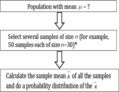
Figure B.1: Process of Sampling Distribution

Note: [* 50 samples each of size n = 30 means that 50 different samples are drawn, where each sample will have 30 items in it. Also, a probability distribution is similar to a frequency distribution. Using the probability distribution, the shape of the sample means is determined].

Example B.1 Examining the Distribution of the Sample Mean

The assembly time of a particular electrical appliance is assumed to have a mean μ = 5 minutes, and a standard deviation σ = 5 minutes.

1. 1.Draw 50 samples each of size 5 (n = 5) from this population using MINITAB statistical software or any other statistical package.
2. 2.Determine the average or the mean of each of the samples drawn.
3. 3.Draw a histogram of the sample means and interpret your findings.
4. 4.Determine the average and standard deviation of the 50 sample means. Interpret the meaning of these.
5. 5.What conclusions can you draw from your answers to (3) and (4)?

Solution to (1): Table B.1 shows 50 samples each of size 5 using MINITAB.

Table B.1: Fifty Samples of Size 5 (n = 5)

Solution to (2): The last column shows the mean of each sample drawn. Note that each row represents a sample of size 5.

Solution to (3): Figure 3.2 shows the histogram of the sample means shown in the last column of Table B.1. The histogram shows that the sample means are normally distributed. Figure B.2 is an example of the sampling distribution of the sample means .

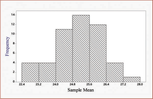
Figure B.2: Sampling Distribution of the Sample Means

In a similar way, we can do the sampling distribution of other statistics such as the sample variance or the sample standard deviation. As we will see later, the sampling distribution provides the distribution or the shape of the sample statistic of interest. This distribution is useful in drawing conclusions.

Solution to (4): The mean and standard deviation of the sample means shown in the last column of Table B.1 were calculated using a computer package. These values are shown in Table B.2.

Table B.2: Mean and Standard Deviation of Sample Means

Descriptive Statistics: Sample Mean
Mean	StDev
25.0942	1.1035

The mean of the sample means is 25.0942, which indicates that values are centered at approximately the population mean of µ = 25.

However, the standard deviation of 50 sample means is 1.1035, which is much smaller than the population standard deviation σ = 3. Thus, we conclude that —or the sample mean—values have much less variation than the individual observations.

Solution to (5): Based on parts (3) and (4), we conclude that the sample mean follows a normal distribution, and this distribution is much narrower than the population of individual observations. This is apparent from the standard deviation of value, which is 1.1035 (see Table B.2). In general, the mean and standard deviation of the random variable are given as follows.

Mean of the sample mean, is

The standard deviation of the sample mean is

For our example, μ = 25, σ = 5, and n = 5. Using these values

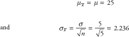
From Table B.2, the mean and the standard deviation of 50 sample means were 25.0942 and 1.1035, respectively. These values will get closer to 25 and 3.0 if we take more and more samples of size 5.

Standard Deviation of the Sample Mean or the Standard Error

Both equations (i) and (ii) are of considerable importance. Equation (ii) shows that the standard deviation of the sample mean (or the sampling distribution of the random variable ) varies inversely as the square root of the sample size. Since the standard deviation of the mean is a measure of the scatter of the sample means, it provides the precision that we can expect of the mean of one or more samples. The standard deviation of the sample mean is often called the standard error of the mean. Using equation (ii), it can be shown that a sample of 16 observations (n = 16) is twice as precise as a sample of 4 (n = 4). It may be argued that the gain in precision in this case is small, relative to the effort in taking additional 12 observations. However, doubling the sample size in other cases may be desirable.

Figure B.3 shows a comparison between the probability distribution of individual observations and the probability distributions of means of samples of various sizes drawn from the underlying population.

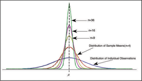
Figure B.3: Probability Distribution of Sample Means (n = 4, 9, 16, and 36) Compared to Individual Observations

Note that as the sample size increases, the standard error becomes smaller and hence the distribution becomes more peaked. It is obvious from Figure B.3 that a sample of one does not tell us anything about the precision of the estimated mean. As more samples are taken, the standard error decreases, thus providing greater precision.

Central Limit Theorem

The other important concept in statistics and sampling is the central limit theorem. The theorem states that as the sample size (n) increases, the distribution of the sample mean () approaches a normal distribution.

This means that if samples of large size (n ≥ 30) are selected from a population, then the sampling distribution of the sample means is approximately normal. This approximation improves with larger samples.

The Central Limit Theorem has major applications in sampling and other areas of statistics. It tells us that if we take a large sample (n ≥ 30), we can use the normal distribution to calculate the probability and draw conclusion about the population parameter.

• •Central Limit Theorem has been proclaimed as “the most important theorem in statistics”¹ and “perhaps the most important result of statistical theory.”
• •The Central Limit Theorem can be proven to show the “amazing result” that the mean values of the sum of a large number of independent random variables are normally distributed.
• •The probability distribution resulting from “a large number of individual effects… would tend to be Gaussian¹ or Normal.”

The above are useful results in drawing conclusions from the data. For a sample size of n = 30 or more (large sample), we can always use the normal distribution to draw conclusions from the sample data.

• •For a large sample, the sampling distribution of the sample mean () follows a normal distribution and the probability that the sample mean () is within a specified value of the population mean (µ) can be calculated using the following formulas:

or

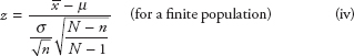
In the above equations, n is the sample size and N is the population size. In a finite population, the population size N is known, whereas in an infinite population, the population size is infinitely large. Equation (iii) is for an infinite population, and equation (iv) is for a finite population.

¹Ostle, Bernard and Mensing, Richard W., Statistics in Research, Third Edition, The Iowa State University Press, Ames, Iowa, 1979, p. 76.

APPENDIX C

Review of Estimation, Confidence Intervals, and Hypothesis Testing

Estimation and hypothesis testing come under inferential statistics. Inferential Statistics is the process of using sample statistics to draw conclusions about the population parameters. Interference problems are those that involve inductive generalizations. For example, we use the statistics of the sample to draw conclusions about the parameters of the population from which the sample was taken. An example would be to use the average grade achieved by one class to estimate the average grade achieved in all ten sections of the same course. The process of estimating this average grade would be a problem of inferential statistics. In this case, any conclusion made about the ten sections would be a generalization, which may not be completely valid, so it must be stated how likely it is to be true.

Statistical inference involves generalization and a statement about the probability of its validity. For example, an engineer or a scientist can make inferences about a population by analyzing the samples. Decisions can then be made based on the sample results. Making decisions or drawing conclusions using sample data raises question about the likelihood of the decisions being correct. This helps us understand why probability theory is used in statistical analysis.

Tools of Inferential Statistics

Inferential tools allow a decision maker to draw conclusions about the population using the information from the sample data. There are two major tools of inferential statistics: estimation and hypothesis testing. Figure C.1 shows the tools of inferential statistic.

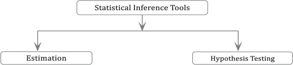
Figure C.1: Tools of Inferential Statistics

• •Estimation is the simplest form of inferential statistics in which a sample statistic is used to draw conclusion about an unknown population parameter.
• •An estimate is a numerical value assigned to the unknown population parameter. In statistical analysis, the calculated value of a sample statistic serves as the estimate. This statistic is known as the estimator of the unknown parameter.
• •Estimation or parameter estimation comes under the broad topic of statistical inference.
• •The objective of parameter estimation is to estimate the unknown population parameter using the sample statistic. Two types of estimates are used in parameter estimation: point estimate and interval estimate.

The parameters of a process are generally unknown; they change over time and must be estimated. The parameters are estimated using the techniques of estimation theory. Hypothesis testing involves making a decision about a population parameter using the information in the sample data. These techniques are the basis for most statistical methods.

Estimation and Confidence Intervals

Estimation

There are two types of estimates: (a) point estimates, which are single-value estimates of the population parameter, and (b) interval estimates or the confidence intervals, which are a range of numbers that contain the parameter with specified degree of confidence known as the confidence level. Confidence level is a probability attached to a confidence interval that provides the reliability of the estimate. In the discussion of estimation, we will also consider the standard error of the estimates, the margin of error, and the sample size requirement.

Point Estimate

As indicated, the purpose of a point estimate is to estimate the value of a population parameter using a sample statistic. The population parameters are μ, σ, p etc.

1. A)The point estimate of the population mean (μ) is the sample mean (),
   
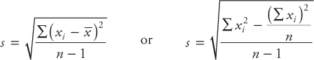
2. B)The point estimate of the population standard deviation (σ) is the sample standard deviation (s)
   
3. C)The point estimate of a population proportion (p) is the sample proportion where x = no. of successes, n = sample size

Interval Estimate

An interval estimate provides an interval or range of values that are used to estimate a population parameter. To construct an interval estimate, we find an interval about the point estimate so that we can be highly confident that it contains the parameter to be estimated. An interval with high confidence means that it has a high probability of containing the unknown population parameter that is estimated.

An interval estimate acknowledges that the sampling procedure is subject to error, and therefore, any computed statistic may fall above or below its population parameter target.

The interval estimate is represented by an interval or range of possible values so it implies the presence of uncertainty. An interval estimate is represented in one of the following ways:

16.8 ≤ µ ≤ 18.6

or

(16.8 to 18.6)

or

(16.8–18.6)

A formal way of writing an interval estimate is “L ≤ µ ≤ U” where L is the lower limit and U is the upper limit of the interval. The symbol µ indicates that the population mean µ is estimated. The interval estimate involves certain probability known as the confidence level.

Confidence Interval Estimate

In many situations, a point estimate does not provide enough information about the parameter of interest. For example, if we are estimating the mean or the average salary for the students graduating with a bachelor’s degree in business, a single estimate that would be a point estimate may not provide the information we need. The point estimate would be the sample average and will just provide a single estimate that may not be meaningful. In such cases, an interval estimate of the following form is more useful:

L ≤ µ ≤ U

It also acknowledges sampling error. The end points of this interval will be random variables since they are a function of sample data.

To construct an interval estimate of unknown parameter β, we must find two statistics L and U such that

The resulting interval L ≤ β ≤ U is called a 100 (1 – α) percent confidence interval for the unknown parameter β. L and U are known as the lower and upper confidence limits, respectively, and (1 – α) is known as the confidence level. A confidence level is the probability attached to a confidence interval. A 95 percent confidence interval means that the interval is estimated with a 95 percent confidence level or probability. This means that there is a 95 percent chance that the estimated interval would include the unknown population parameter being estimated.

Interpretation of Confidence Interval

The confidence interval means that if many random samples are collected and a 100 (1−α) percent confidence interval computed from each sample for β, then 100 (1−α) percent of these intervals will contain the true value β.

In practice, we usually take one sample and calculate the confidence interval. This interval may or may not contain the true value, and it is not reasonable to attach a probability level to this specific event. The appropriate statement would be that β lies in the observed interval [L,U] with confidence 100(1−α). That is, we don’t know if the statement is true for this specific sample, but the method used to obtain the interval [L,U] yields correct statement 100 (1−α) percent of the time. The interval L ≤ β ≤ U is known as a two-sided or two-tailed interval. We can also build one-sided interval. The length of the observed confidence interval is an important measure of the quality of information obtained from the sample. The half interval (β – L) or (U – β) is called the accuracy of the estimator. A two-sided interval can be interpreted in the following way:

The wider the confidence interval, the more confident we are that the interval actually contains the unknown population parameter being estimated. On the other hand, the wider the interval, the less information we have about the true value of β. In an ideal situation, we would like to obtain a relatively short interval with high confidence.

Confidence interval for the mean, known variance σ² (or σ known)

The confidence interval estimate for the population mean is centered around the computed sample mean (). The confidence interval for the mean is constructed based on the following factors:

1. A)The size of the sample (n),
2. B)The population variance (known or unknown), and
3. C)The level of confidence.

Let X be a random variable with an unknown mean µ and known variance σ². A random sample of size n (x₁, x₁,...,x_n) is taken from the population. A 100 (1 – α) percent confidence interval on µ can be obtained by considering the sampling distribution of the sampling mean . We know that the sample mean follows a normal distribution as the sample size n increases. For a large sample n the sampling distribution of the sample mean is almost always normal. The sampling distribution is given by:

The distribution of the above is normal and is shown in Figure C.2. To develop the confidence interval for the population mean µ, refer to Figure C.2.

Figure C.2: Distribution of the Sample Mean

From the above figure we see that:

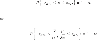
This can be rearranged to give:

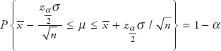
This leads to:

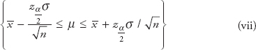
Equation (vii) is a 100(1−α) percent confidence interval for the population mean µ.

The confidence interval formula to estimate the population mean µ for known and unknown population variances or standard deviations

The confidence interval is constructed using a normal distribution. The following two formulas are used when the sample size is large:

1. A)Known population variance (σ²) or known standard deviation (σ)

Note that the margin of error is given by

1. B)Unknown population variance (σ²) or unknown standard deviation (σ)
   
2. C)Unknown population variance (σ²) or unknown standard deviation (σ)

If the population variance is unknown and the sample size is large, the confidence interval for the mean can also be calculated using a normal distribution using the following formula:

In the above confidence interval formula, s is the sample standard deviation.

Confidence interval for the mean when the sample size is small and the population standard deviation σ is unknown

When σ is unknown and the sample size is small, use t-distribution for the confidence interval. The t-distribution is characterized by a single parameter, the number of degrees of freedom (df), and its density function provides a bell-shaped curve similar to a normal distribution.

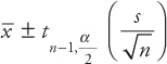
The confidence interval using t-distribution is given by

where t _n−1,α/2 = t-value from the t-table for (n₋1) degrees of freedom and α/2 where α is the confidence level.

Confidence interval for estimating the population proportion p

In this section, we will discuss the confidence interval estimate for the proportions. A proportion is a ratio or fraction, or percentage that indicates the part of the population or sample having a particular trait of interest. Following are the examples of proportions: (1) a software company claiming that its manufacturing simulation software has 12 percent of the market share, (2) a public policy department of a large university wants to study the difference in proportion between male and female unemployment rate, and (3) a manufacturing company wants to determine the proportion of defective items produced by its assembly line. In all these cases, it may be desirable to construct the confidence intervals for the proportions of interest. The population proportion is denoted by “p,” whereas the sample proportion is denoted by .

In constructing the confidence interval for the proportion:

1. 1.The underlying assumptions of binomial distribution holds.
2. 2.The sample data collected are the results of counts (e.g., in a sample of 100 products tested for defects, 6 were found to be defective).
3. 3.The outcome of the experiment (testing 6 products from a randomly selected sample of 100 is an experiment) has two possible outcomes—“success” or “failure” (a product is found defective or not).
4. 4.The probability of success (p) remains constant for each trial.

We consider the sample size (n) to be large. If the sample size is large and

[where n = sample size, p = population proportion], the binomial distribution can be approximated by a normal distribution. In constructing the confidence interval for the proportion, we use large sample size so that normal distribution can be used.

The confidence interval is based on:

1. A)The large sample so that the sampling distribution of the sample proportion follows a normal distribution.
2. B)The value of sample proportion.
3. C)The level of confidence, denoted by z.

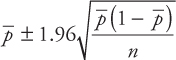
The confidence interval formula is given by:

In the above formula, note that

p = population proportion and is the sample proportion given by .

Sample Size Determination

Sample size (n) to estimate µ

Determining the sample size is an important issue in statistical analysis. To determine the appropriate sample size (n), the following factors are taken into account:

1. A)The margin of error E (also known as tolerable error level or the accuracy requirement). For example, suppose we want to estimate the population mean salary within $500 or within $200. In the first case, the error E = 500; in the second case, E = 200. A smaller value of the error E means more precision is required, which in turn will require a larger sample. In general, smaller the error, larger the sample size.
2. B)The desired reliability or the confidence level.
3. C)A good guess for σ.

Both the margin of error E and reliability are arbitrary choices that have an impact on the cost of sampling and the risks involved. The following formula is used to determine the sample size:

E = margin of error or accuracy (or maximum allowable error), n = sample size

Sample size (n) to estimate p

The sample size formula to estimate the population proportion p is determined similar to the sample size for the mean. The sample size is given by

p = population proportion (if p is not known or given, use p = 0.5).

Example C.1

A quality control engineer is concerned about the bursting strength of a glass bottle used for soft drinks. A sample of size 25 (n = 25) is randomly obtained, and the bursting strength in pounds per square inch (psi) is recorded. The strength is considered to be normally distributed. Find a 95 percent confidence interval for the mean strength using both t-distribution and normal distribution. Compare and comment on your results.

Data: Bursting Strength (×10 psi)

26, 27, 18, 23, 24, 20, 21, 24, 19, 27, 25, 20, 24, 21, 26, 19, 21, 20, 25, 20, 23, 25, 21, 20, 21

Solution:

First, calculate the mean and standard deviation of 25 values in the data. You should use your calculator or a computer to do this. The values are

= 22.40

S = 2.723

The confidence interval using a t-distribution can be calculated using the following formula:

A 95 percent confidence interval using the above formula:

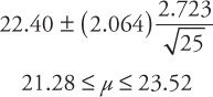
The value 2.064 is the t-value from the t-table for n−1 = 24 degrees of freedom and α/2 = 0.025.

The confidence interval using a normal distribution can be calculated using the formula below:

This interval is

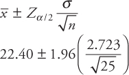
The confidence interval using the t-distribution is usually wider. This happens because with smaller sample size, there is more uncertainty involved.

Example C.2

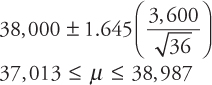
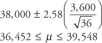
The average life of a sample of 36 tires of a particular brand is 38,000 miles. If it is known that the average lifetime of the tires is approximately normally distributed with a standard deviation of 3,600 miles, construct 80 percent, 90 percent, 95 percent, and 99 percent confidence intervals for the average tire life. Compare and comment on the confidence interval estimates.

Solution: Note the following data:

Since the sample size is large (n ≥ 30), and the population standard deviation σ is known, the appropriate confidence interval formula is

The confidence intervals using the above formula are shown below.

1. A)80 percent confidence interval

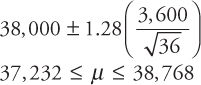
1. B)90 percent confidence interval

1. C)95 percent confidence interval

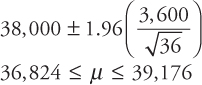
1. D)99 percent confidence interval

Note that the z-values in the above confidence interval calculations are obtained from the normal table. Refer to the normal table for the values of z. Figure C.3 shows the confidence intervals graphically.

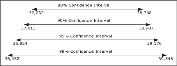
Figure C.3: Effect of Increasing the Confidence Level on the Confidence Interval

Figure C.3 shows that larger the confidence level, the wider is the length of the interval. This indicates that for a larger confidence interval, we gain confidence. There is higher chance that the true value of the parameter being estimated is contained in the interval but at the same time, we lose accuracy.

Example C.3

During an election year, ABC news network reported that according to its poll, 48 percent voters were in favor of the democratic presidential candidate with a margin of error of ±3 percent. What does this mean? From this information, determine the sample size that was used in this study.

Solution: The polls conducted by the news media use a 95 percent confidence interval unless specified otherwise. Using a 95 percent confidence interval, the confidence interval for the proportion is given by

The sample proportion, = 0.48. Thus, the confidence interval can be given by

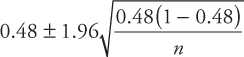
Since, the margin of error is ±3 percent, it follows that

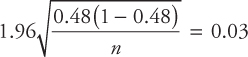
Squaring both sides and solving for n gives

n = 1066

Thus, 1066 voters were polled.

Example C.4

A pressure seal used in an assembly must be able to withstand a maximum load of 6,000 psi before bursting. If the average maximum load of a sample of seals taken from a shipment is less than 6,000 psi, then the quality control must reject the entire shipment. How large a sample is required if the quality engineer wishes to be 95 percent confident that the error in estimating this quantity is no more than 15 psi, or the probability that the sample mean differs from the population mean by no more than 15 psi is 0.95. From the past experience, it is known that the standard deviation for bursting pressures of this seal is 150 psi.

Solution: The sample size n can be calculated using

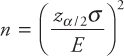
Since Z_α/2 = Z_0.025 = 1.96, σ = 150, and the error E = 15, the required sample size will be as follows:

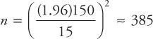
Confidence Interval on the Difference between Two Means

The confidence interval discussed in the previous sections involved a single population. In many cases, we are interested in comparing two populations. Suppose the average hourly wage of union and nonunion workers is of interest. We are interested to find out whether there is a difference in the wages between the two. In this case, we would construct a confidence interval on the difference between the two means. These intervals depend on what information is available. The different cases are explained below.

Case 1

Assumptions:

• •the two populations are independent.
• •the population variances are equal.
• •the samples n₁ and n₂ are large and population variances σ₁² and σ₂² are known so that normal distribution applies.

If the above assumptions hold, then the confidence interval for the difference between two population means is given by

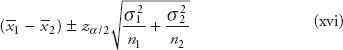
or

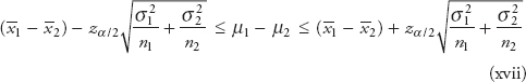
where are the sample means from populations 1 and 2

n₁, n₂ = sample size of samples 1 and 2

= variances of 1st and 2nd populations, respectively (known in this case)

Case 2

Assumptions:

• •the two populations are independent;
• •the population variances are equal;
• •the samples n₁ and n₂ are large and population variances σ₁² and σ₂² are unknown, which means the normal distribution can be applied.

If the above assumptions hold, then the confidence interval for the difference between two population means is given by

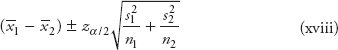
or

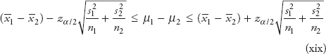
where s₁² and s₂²= sample variances of 1st and 2nd sample, respectively

= sample means from populations 1 and 2, respectively

n₁, n₂ = sample size of samples 1 and 2

Case 3

Assumptions:

• •the two populations are independent;
• •the population variances are equal;
• •the samples n₁ and n₂ are small (<30) and population variances σ₁² and σ₂² are unknown so that t-distribution applies.

If the above assumptions hold, then the confidence interval for the difference between two population means is given by

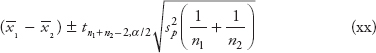
or

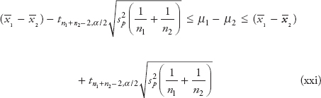
where = sample means from populations 1 and 2, respectively

n₁, n₂ = sample size of sample, 1 and 2

s₁², s₂² = sample variances of 1st and 2nd sample, respectively

n₁+ n₂ – 2 = degrees of freedom

s_p² is the “pooled” or combined variance, given by

Note: in this problem, first calculate s_p² and then substitute in equation to calculate the confidence interval.

Example C.4

The average hourly wage of union and nonunion workers is of interest. Assume that (i) the populations are independent and (ii) the variances of the populations are equal (σ₁² = σ₂²). Sample from both groups were taken with the following results:

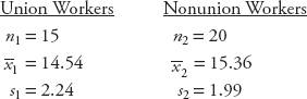
1. A)Find the “pooled” estimate of the variance.

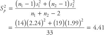
1. B)Find a 95 percent confidence interval for the difference in the mean hourly wage.
   Confidence interval formula for this case:

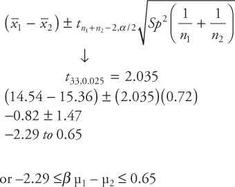
Note that this interval contains zero (–2.29 to 0.65). This means that the difference is zero at some point in the interval, indicating there is no difference in the average wage of union and nonunion workers.

Point and Interval Estimates for the Difference between Two Population Proportions

Consider two large populations. Let p₁ and p₂ denote the proportions of these two populations that have certain characteristic of interest. Suppose we want to find the difference between the two population proportions. To do this, we will take two random samples of size n₁ and n₂ from the two populations. If x₁ is the number having the characteristic of interest in the first population and x₂ the number having the characteristic of interest in the second population, then and are the sample proportions of the two samples that have the characteristic of interest. Note that

The point estimate for the difference between the population proportions is given by

The confidence interval for the difference between the population proportions is given by

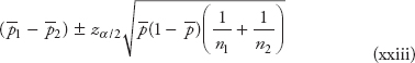
where () is the “pooled” or combined proportion given by

Example C.5

A manufacturer of computer chips has two plants in two different cities. An improved method of producing the chips is suggested by the research and development department which is expected to reduce the proportion of defective chips. After implementing the new method in one of the plants, the manufacturer wanted to test whether the improved method actually reduced the proportion of defects. To do this, they collected a sample of 400 chips from the improved method of production and a sample of 450 chips from the old production method. The numbers of defective chips were found to be 80 and 108, respectively. At a 95 percent confidence, can we conclude that there is a difference in proportion of defective chips?

Proportion of defective using the improved method:

Proportion of defective using the old method: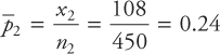

Combined or the “pooled” proportion:

The confidence interval:

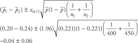
Thus, a 95 percent confidence interval is

-0.1 ≤ p₁ - p₂ ≤ 0.02

This interval contains zero, which indicates that there is no difference between the improved method and the old method of production.

APPENDIX D

Hypothesis Testing for One and Two Population Parameters

Hypothesis Testing

A hypothesis is a statement about a population parameter. This statement may come from a claim made by a manufacturer, a mathematical model, a theory, design specifications, etc. For example, an automobile manufacturer may claim that they have come up with a new fuel injection system design that provides an improved average mileage of 50 miles a gallon. In such a case, we may want to test the claim by taking sample data. The claim can formally be written as a hypothesis testing problem and can be tested using a hypothesis testing procedure. Several population parameters may be of interest. Sometimes we may be interested in testing the average or the mean. In other cases, we may be interested in testing a variance, a standard deviation, or a population proportion.

Many problems require us to decide whether or not a statement about some parameter is true or false. This statement about the population parameter is called a hypothesis.

Hypothesis testing is the decision-making procedure about a statement being true or false. The statement is about a population parameter of interest, such as a population mean, population variance, or a population proportion. It involves making a decision about a population parameter based on the information contained in the sample data.

Hypothesis testing is one of the most useful aspects of statistical inference because many types of decision problems can be formulated as hypothesis testing problems.

The control charts used in statistical process control are closely related to the hypothesis testing. The tests are also used in several quality control problems and form the basis of many of the statistical process techniques to be discussed in the coming chapters.

Example D.1: Testing a Single Population Mean—An Example

An automobile manufacturer claims that their new hybrid model will provide 60 miles per gallon on average because of an improved design. A consumer group wants to test whether this claim is correct. They would test a hypothesis stated formally as follows:

H0: μ = 60mpg

H1: μ ≠ 60mpg

Here, H₀ is known as the null hypothesis and H₁ (also written H_a) is called the alternate hypothesis. The hypothesis written with an “equal to” sign under the null hypothesis and a “not equal to” sign under the alternate hypothesis is known as a two-sided or two-tailed test. A hypothesis can also be one-sided or one-tailed. The alternate hypothesis is opposite of the null hypothesis. To test the validity of the above claim,

• •The consumer group would gather the sample data and calculate the sample mean, .
• •Compare the difference between the hypothesized value (µ) and the value of the sample mean ().
• •If the difference is small, there is a greater likelihood that the hypothesized value of the population mean is correct. If the difference is large, there is less likelihood that the claim about the population mean is correct.

In most cases, the difference between the hypothesized population parameter and the actual sample statistic is neither so large that we reject our hypothesis nor is it so small that we accept it. Thus, in hypothesis testing, clear-cut solutions are not the rule.

Note that in hypothesis testing, the decision to reject or not to reject the hypothesis is based on a single sample and therefore, there is always a chance of not rejecting a hypothesis that is false, or rejecting a hypothesis that is true. In fact, we always encounter two types of errors in hypothesis testing. These are:

Type I error = α = P {Reject H₀ ∙ H₀ is true}

Type II error = β = P {Fail to reject H₀ ∙ H₀ is false}(i)

We also use another term known as the power of the test defined as

Power = 1 – β = P {Reject H₀ ∙ H₀ is false}

Thus, type I error, denoted by a Greek letter α (“alpha”), is the probability of rejecting a true null hypothesis and type II error, denoted by a Greek letter β (“beta”), is the probability of not rejecting a null hypothesis when it is false. In a hypothesis testing situation, there is always a possibility of making one of these errors.

The power of the test is the probability that a false null hypothesis is correctly rejected. Type I error α is selected by the analyst. Increasing the type I error α will decrease the type II error β and decreasing the type I error α error will increase the type II error β. Thus, the type I error is controlled by the analyst and the type II error is determined based on the type I error. The type II error is a function of the sample size. The larger the sample size n, the smaller is the β.

The type I error α is also known as the level of significance. In hypothesis testing, we specify a value of the type I error or the level of significance and then design a test that will provide a small value of the type II error. Recall that the type I error is the probability of rejecting a true null hypothesis. Since we don’t want this to happen, α is set to a low value of 1 percent, 5 percent or 10 percent in general cases. If you set the value of α = 5 percent, it means that there is a 5 percent chance of making an incorrect decision, and a 95 percent chance of making a right decision. In a hypothesis testing, there is never a 100 percent chance of making a right decision because the test is based on one sample (large or small).

What does it mean to test a hypothesis at a 5 percent level of significance?

Suppose we want to test a hypothesis about a population mean and the sample size is large (n ≥ 30) so that the sample mean follows a normal distribution. If the level of significance α is set at 5 percent, it means that we will reject the null hypothesis if the difference between the sample statistic (in this case, ) and the hypothesized population mean µ is so large that it would occur on the average only 5 or fewer times in every 100 samples. See Figure D.1. This figure shows that if the sample statistic falls in the “do not reject” area, we will not reject the null hypothesis. On the other hand, if the sample value falls in the rejection areas, we will reject the null hypothesis. Rejecting the null hypothesis means that the alternate hypothesis is true.

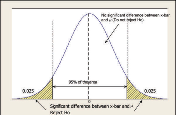
Figure D.1: Rejection and Nonrejection Areas

It is evident from the figure that by selecting a significance level α, the areas of rejection and nonrejection are determined. In other words, we set the boundaries that determine when to reject and when not to reject the null hypothesis.

Note that the value of α is selected by the analyst and it must be determined before you conduct the test. If we don’t have a significance level α, we don’t know when to reject and when not to reject a hypothesis.

In a hypothesis testing situation, there is always a possibility of making one of the two types of errors (i.e., there is always a chance of rejecting a true null hypothesis; similarly, there is always a chance of accepting a false null hypothesis). In hypothesis testing, we must consider the cost and the risk involved in making a wrong decision. Also, we would like to minimize the chance of making either a type I or type II error; therefore, it is desirable to have the probabilities of both type I and type II error to be low.

In quality control, α is also known as producer’s risk because it denotes the probability of rejecting a good lot. The type II error β is referred as the consumer’s risk as it indicates the probability of accepting a bad lot.

Testing a single population mean

Testing a population mean involves testing a one-sided or a two-sided test. The hypothesis is stated as:

H0: μ = μ0 H1: μ ≠μ0 Two-tailed or two-sided test

H0: μ ≥ μ0 H1: μ < μ0 Left-tailed or left-sided test

H0: μ ≤ μ0 H1: μ > μ0 Right-tailed or right-sided test

Note that μ₀ is the hypothesized value. There are three possible cases for testing the population mean. The test statistic or the formulas used to test the hypothesis are given below.

Case (1): Testing a single mean with known variance or known population standard deviation σ and large sample: in this case, the sample mean follows a normal distribution and the test statistic is given as follows:

Case (2): Testing a single mean with unknown variance or unknown population standard deviation σ and large sample: in this case, the sample mean follows a normal distribution and the test statistic is given by

Case (3): Testing a single mean with unknown variance or unknown population standard deviation σ and small (n < 30) sample. In this case, the sample mean follows a t-distribution and the test statistic is given by

Note that s is the sample standard deviation and n is the sample size.

There are different ways of testing a hypothesis. These will be illustrated with examples.

Example D.2 Formulating the Correct Hypothesis

A hypothesis test can be formulated as a one-sided or a two-sided test. If we have a one-sided test, it can be a left-sided or a right-sided test.

Example of a left-sided test

Suppose a tire manufacturer claims that the average mileage provided by a certain type of tire is at least 60,000 miles. A product research group has received some complaints in the past and wants to check the claim. They are interested in testing whether the average mileage is below 60,000 miles. They would formulate their hypothesis as follows:

The hypothesis is formulated as shown above because the claim of at least 60,000 miles is µ ≥ 60,000 and the opposite of this statement is µ < 60,000 miles. Since the null hypothesis is written with an “equal to” sign, and this is the claim made by the manufacturer, the statement µ ≥ 60,000 is written under the null hypothesis, and the statement µ < 60,000 is written under the alternate hypothesis.

Note that the alternate hypothesis is opposite of the null hypothesis. This is an example of a left-sided test. The left-sided test will reject the null hypothesis (H₀) below a specified hypothesized value of µ.

The alternate hypothesis is also known as the research hypothesis. If you are trying to establish a certain hypothesis, then it should be written as the alternate hypothesis.

The statement about the null hypothesis contains the claim or the theory. Therefore, rejecting a null hypothesis is a strong statement. This is the reason that the conclusion of a hypothesis test is stated as “reject the null hypothesis” or “do not reject the null hypothesis.”

Example of a right-sided test:

A car manufacturer has made a significant improvement in the fuel injection system that is expected to provide an improved gas mileage. The average mileage before the modification was 24 miles or less. The research group expects that the modified system will provide significant improvement in the gas mileage. The group would like to test the following hypothesis to show the improvement:

Example of a two-sided test

A robot welder in an assembly line takes on average 1.5 minutes to finish a welding job. If the average time taken to finish the job is higher or lower than 1.5 min, it will disrupt other activities along the production line. Since there has been too much variation in the time it takes to perform the welding job by the robot, the line supervisor wants to take a sample to check if the average time taken by the robot is significantly higher or lower than the average of 1.5 minutes. The supervisor would be testing the following hypothesis:

Example D.3

A new production method will be implemented if a hypothesis test supports the conclusion that the new method results in reduced production cost per hour. If the current average operating cost per hour is $600 or more, write the appropriate hypothesis. Also, state and explain the type I and type II errors in this situation.

1. A)Write the appropriate null and alternate hypotheses.
   The appropriate hypotheses to test the claim:

1. B)State and explain the type I and type II errors in this situation.
   Type I error: Reject H₀: µ ≥ 600 and conclude that the average production cost is less than $600 (µ < $600). Type II error would be to conclude that the average operating cost is at least $600 when it is not.

Example D.4

In a production line, automated machines are used to fill beverage cans with an average fill volume of 16 ounces. If the mean weight falls above or below this figure, the production line must be stopped and some remedial action be taken. A quality control inspector samples 30 cans every hour, opens and weighs the content, tests the appropriate hypothesis, and makes a decision whether to shut down the line for making adjustments. Write the appropriate hypothesis to be tested in this situation and perform the hypothesis test. A significance level of α = 0.05 is selected for the test. The sample results indicate a sample mean of 16.32 oz and the standard deviation is assumed to be 0.8 oz.

Solution: For this problem, the given data are:

n = 30, α = 0.05

1. 1.State the null and alternate hypothesis

Note that this is a two-sided test.

1. 2.Determine the sample size or use the given sample size

The given sample size is n = 30 (large sample)

1. 3.Determine the appropriate level of significance (α) or use the given value of significance, α

The given level of significance α = 0.05

1. 4.Select the appropriate distribution and test statistic to perform the test
   The sample size is large and the population standard deviation is known; therefore, use normal distribution with the following test statistic:

1. 5.Based on step 3, find the critical value or values and the area or areas of rejection. Show the critical value(s) and the area or areas of rejection and non rejection using a sketch
   This is a two-sided test. The level of significance α = 0.05 must be split into two halves for a two-tailed test, with each tail area 0.025. The critical value (z-value) for an area of 0.475 is 1.96 from the normal or z-table. The sketch is shown in Figure D.2.
2. 6.Write the decision rule

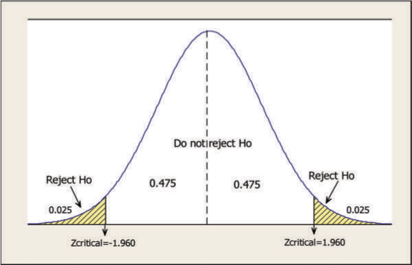
Figure D.2: Critical Values for a Two-Sided Test

Reject H₀ if z > 1.96
or, if z < –1.96

1. 7.Use the test data (sample data) and find the value of the test statistic

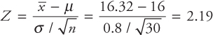
1. 8.Find out if the value of the test statistic is in rejection or non rejection region; make appropriate decision and state your conclusion in terms of the problem

z = 2.19 > Z_critical = 1.96; therefore, reject H₀

There is an evidence of overfilling or underfilling. The line should be shut down.

Example D.5: Testing the hypothesis using the p-value approach

In the z-value approach of testing the hypothesis, we compared the test statistic value to the critical value of z to either reject or not to reject the hypothesis. For example, in the previous example, the critical value z was ±1.96 and the test statistic value was 2.19. Since the test statistic value of 2.19 is greater than the critical value of +1.96, we rejected the null hypothesis. In this method of testing the hypothesis, we compared similar terms (test statistic value of z to the critical z-value). This method of stating the conclusion in the hypothesis test requires a predefined level of significance, which may not tell us if the computed test statistic value is barely in the rejection region or it is far into the region. In other words, the information may be inadequate sometimes.

To overcome this problem, another approach of testing the hypothesis is suggested, which is widely used in testing hypothesis. This is known as p-value (probability value) approach. This method compares a probability to the given probability.

You may recall that to test a hypothesis you must have the level of significance α, which is decided by the analyst before conducting the test. This α is the same as the type I probability and is often called the given level of significance. In a hypothesis testing situation, the type I probability is given or known. We then calculate the p-value or the probability based on the sample data. This is also the observed level of significance. We then compare the given level of significance α to the p-value (observed level of significance) to test and draw the conclusion about the hypothesis.

The p-value is the probability (assuming that the null hypothesis is true) of getting the value of the test statistic at least as extreme as or more extreme than the value actually observed. The p-value is the smallest level of significance at which the null hypothesis can be rejected. A small p-value for example, p = 0.05 or less, is a strong indicator that the null hypothesis is not true. The smaller the value of p, the greater the chance that the null hypothesis is false.

If the computed p-value is smaller than the given level of significance α, the null hypothesis H₀ is rejected. If the p-value is greater than α then H₀ is not rejected. For example, a p-value of 0.002 indicates that there is less chance that H₀ is true, while a p-value of 0.2356 indicates a less likelihood of H₀ being false. The p-value also provides us insight into the strength of the decision. This tells us how confident we are in rejecting the null hypothesis.

Example D.6: Testing the hypothesis using p-value approach

We will test the hypothesis using p-value for the following two-sided test:

The data for the problem: n = 50, = 14.2, s = 5, α = 0.02

Decision rule for p-value approach

If p ≥ α, do not reject H₀
If p < α; reject H₀

First, using the appropriate test statistic formula, calculate the test statistic value.

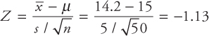
This test statistic value of z = –1.13 will be converted into a probability that we call p-value. This is shown in Figure D.3.

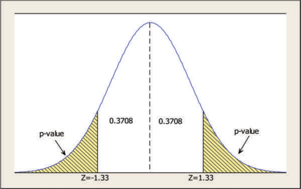
Figure D.3: p-Values for the Example Problem

Area corresponding to z = 1.13 is 0.3708 (from z-table).

Probability of z > 1.13 = 0.5 – 0.3708 = 0.1292
Probability of z < –1.13 = 0.5 – 0.3708 = 0.1292

For a two-sided test, the p-value is the sum of the above two values, that is, 0.1292+0.1292 = 0.2584. Since p = 0.2584 > α = 0.02, do not reject H₀.

Hypothesis Testing Involving Two Population Means

Hypothesis Testing Involving Two Population Means

This section extends the concepts of hypothesis testing to two populations. Here we are interested in testing two population means. For example, we may be interested in comparing the average salaries of male and female employees for the same job or we may be interested in the difference between the average starting salaries of business and engineering majors. In these cases, we would like to test whether the two population means are equal or there is no difference between the two populations (two-sided test). In other cases, we may want to test if one population is larger or smaller than the other population (one-sided test). The hypothesis testing procedures or steps are very similar to those for testing the single mean but the data structure and the test statistic or the formulas to test these hypotheses are different. In testing hypothesis involving two populations, the samples will be drawn from both populations. The hypotheses tested are explained below.

Hypothesis testing for the equality of two means or the differences between two population means

Basic Assumptions:

1. 1.The populations are independent
2. 2.The population variances are equal (σ₁² = σ₂²)

The hypothesis for testing the two means can be a two-sided test or a one-sided test. The hypothesis is written in one of the following ways:

1. A)Test if the two population means are equal or there is no difference between the two means: a two-sided test

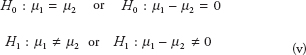
1. B)Test if one population mean is greater than the other: a right-sided test

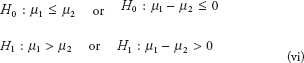
1. C)Test if one population mean is smaller than the other: a left-sided test

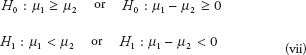
Since we want to study two population means, the sampling distribution of interest is the sampling distribution of the difference between the sample means and the test statistic is based on the information (data) we have. The following three cases and test statistics are used to test the means. To test two means, the test statistics are selected based on the following cases:

Case 1: Sample sizes n₁ and n₂ are large (≥ 30) and the population variances σ₁² and σ₂² are known

If the sample sizes n₁ and n₂ are large (≥ 30) and the population variances σ₁² and σ₂² are known, then the sampling distribution of the difference between the sample means follows a normal distribution and the test statistic is given by

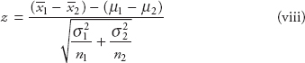
where = sample means from populations 1 and 2, respectively

n₁, n₂ = sample size of samples 1 and 2

σ₁², σ₂² = variances of 1st and 2nd populations, respectively (known in this case)

Case 2: Sample sizes n₁ and n₂ are large (≥ 30) and the population variances σ₁² and σ₂² are unknown

If the sample sizes n₁ and n₂ are large (≥ 30) and the population variances σ₁² and σ₂² are unknown, then the sampling distribution of the difference between the sample means follows a normal distribution and the test statistic is given by

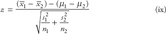
where = sample means from populations 1 and 2, respectively

n₁, n₂ = sample size of samples 1 and 2

s₁², s₂² = sample variances of 1st and 2nd sample, respectively

Case 3: Sample sizes n₁ and n₂ are small (≥ 30) and the population variances σ₁² and σ₂² are unknown

If the sample sizes n₁ and n₂ are small (≥ 30) and the population variances σ₁² and σ₂² are unknown, then the sampling distribution of the difference between the sample means follows a t-distribution and the test statistic is given by

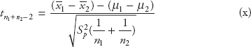
where = sample means from populations 1 and 2, respectively

n₁, n₂ = sample size of samples 1 and 2

s₁², s₂² = sample variances of 1st and 2nd sample, respectively

n₁+ n₂ –2 = degrees of freedom (df)

s_p² is the “pooled” or combined variance, given by

Important Note:

In the equations (viii), (ix) and (x) the difference (µ₁ - µ₂) is zero in most cases. Also, these equations are valid under the following assumptions:

• •The populations are independent and normally distributed
• •The variances of the two populations are equal; that is, (σ₁² = σ₂²)

The assumption that the two population variances are equal may not be correct. In cases where the variances are not equal, the test statistic formula for testing the difference between the two means is different.

Example D.6

Suppose that two independent random samples are taken from two processes with equal variances and we would like to test the null hypothesis that there is no difference between the means of two processes or the means of the two processes are equal; that is,

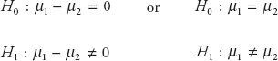
The data from the two processes are given below:

Note that when n₁, n₂ are large and σ₁, σ₂ are unknown, therefore use normal distribution. The test statistic for this problem is

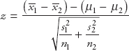
Solution: The test can be done using four methods that are explained below.

Method (1): z-Value Approach

Critical values: The critical values and the decision areas based on α = 0.05 are shown in Figure D.4. Decision Rule:

Reject H₀ if z > 1.96
or if z < –1.96

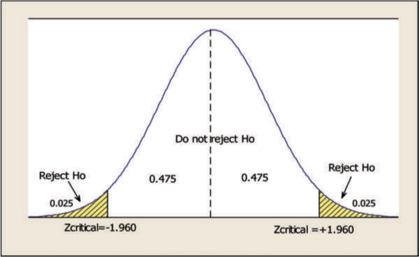
Figure D.4: Critical Values and Decision Areas

Test Statistic Value:

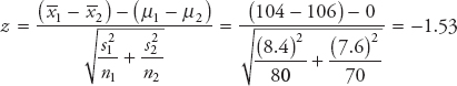
The test statistic value z –1.53 > Z_critical = –1.96; do not reject H₀.

Method (2): p-value Approach

Calculate the p-value and compare it to α. Note that in this method we compare a probability to a probability; that is, we compare the given level of significance α or the type I probability to the probability obtained from the data (or the observed level of significance). The decision rule and the procedure are explained below.

Calculating p-value: The p-value is calculated by converting the test-statistic value into a probability. In method (1), we calculated the test statistic value z. This value was –1.53 or z = –1.53. This test statistic value is converted to a probability (see Figure D.5).

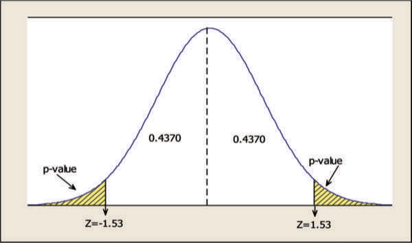
Figure D.5: p-Values

In the above figure, z = 1.53 is the test statistic value from method 1 above.

From the standard normal table, z = 1.53 corresponds to 0.4370. The p-value is calculated as shown below.

Probability of z > 1.53 = 0.5 – 0.4370 = 0.0630
Probability of z < –1.53 = 0.5 – 0.4370 = 0.0630

In a two-sided test such as this one, the p-value is obtained by adding the probabilities in both tails of the distribution. Thus,

p = 0.0630 + 0.0630 = 0.1260

Since p(= 0.1260 > α(= 0.05), do not reject H_0.

Testing Two Means for Dependent (Related) Populations or Hypothesis Testing for Paired Samples (Paired t-Test)

In some situations, there may be a relationship between the data values of the samples of two populations and the data values or the sample values from one population may not be independent of the sample values from the other population. The two populations may be considered dependent in such cases.

In cases where the populations are considered related, the observations are paired to prevent other factors from inflating the estimate of the variance. This method is used to improve the precision of comparisons between means. The method of testing the difference between the two means when the populations are related is also known as matched sample test or the paired t-test.

We are interested in testing a two-sided or a one-sided hypothesis for the difference between the two population means. The hypotheses can be written as

Two-tailed or two-sided test

Right tailed or right-sided test

Left-tailed or left-sided test

Note: the difference d can be taken in any order (sample 1-sample 2) or (sample 2-sample1).

Test Statistic: If the pairs of data values X_1n and X_2n are related and are not independent, the average of the differences () follows a t-distribution and the test statistic is given by

where

= average of the differences

S_d = standard deviation of the differences

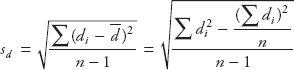
n = number of observations (sample size)

= critical t-value from the t-table for (n – 1) degrees of freedom and appropriate α

The confidence interval given below can also be used to test the hypothesis

Summary

This section discussed three important topics that are critical to analytics. In particular, we studied sampling and sampling distribution, estimation and confidence intervals, and hypothesis testing. Samples are used to make inferences about the population and this can be done through sampling distribution. The probability distribution of a sample statistic is called its sampling distribution. We explained the central limit theorem and its role in sampling, sampling distribution, and sample size determination. Besides sampling and sampling distribution, other key topics covered included point and confidence interval estimates of means and proportions.

Two types of estimates used in inferential statistics were discussed. These estimates include (a) point estimates, which are single-value estimates of the population parameter, and (b) interval estimates or the confidence intervals, which are a range of numbers that contain the parameter with specified degree of confidence known as the confidence level. Confidence level is a probability attached to a confidence interval that provides the reliability of the estimate. In the discussion of estimation, we also discussed the standard error of the estimates, the margin of error, and the sample size determination.

We also discussed the concepts of hypothesis testing, which is directly related to the analysis methods used in analytics. Hypothesis testing is one of the most useful aspects of statistical inference. We provided several examples on formulating and testing hypothesis about the population mean and population proportion. Hypothesis tests are used in assessing the validity of regression methods. They form the basis of many of the assumptions underlying the analytical methods to be discussed in this book.