CHAPTER 2

An Introduction to Data Science/AI for the Nontechnical Person

In this chapter we will delve deeper into data science, and discuss what it is, and why it’s useful. We will cover the brief history of data science and take a look at the core fields that compose it. The aim of this chapter is to give to the nontechnical reader a good brief overview of that area and understand where it can be applied and why.

Data science is made up of multiple disciplines. So, to get a good grasp of what data science is, we need to look at the core disciplines that make up this field of study. First, though, let’s take a quick look at how it all started.

Brief History of Data Science

Though data science became more popular with the increase of data generation, it has been around for a while. Many look to John Tukey as one of the people who pushed the boundaries of statistics and gave birth to the concept of data analysis as a science (Leonhardt 2000).

Tukey wrote The Future of Analysis in 1962, while he was a professor at Princeton University and working at Bell Labs to develop statistical methods for computers (Tukey 1962).

In the article, he encouraged academic statisticians to get involved in the entire process of data analysis instead of just focusing on statistical theory. He pointed out how important it was to distinguish between exploratory and confirmatory data analysis, which was the first step to creating the field of data science.

While others certainly had a significant impact on data science as we know it today, Tukey was among the first to advocate for the importance of such a field. However, it took some time until the early 2000s for data science to really take off. The reason is that the turn of the millennium saw a few trends converging:

1. The rise of the Internet;

2. Cheaper storage and computing power;

3. The rise of cloud computing;

4. The rise in the volumes of data being generated.

The convergence of those four trends made data a valuable resource, with some calling data the new oil. This incentivized the re-emergence of the field of data science as a unifying force into what used to be disparate fields.

The Core Fields of Data Science

Taking a closer look at the history of data science means delving into its three core fields: AI, ML, and statistics. There are many other trends that have risen and fallen over the years: data mining, pattern recognition, cybernetics, and more. These terms often describe scientific approaches that tried to recreate intelligence inside a machine, or developed techniques to extract insights from data. However, the primary fields are AI, ML, and statistics, and we will delve into these in more depth over the next few chapters.

A Closer Look at AI

AI is exactly what it sounds like. People are trying to get machines to think like humans. In more technical terms, this means giving a machine the ability to reason logically, self-correct, and learn. Written out as it is, it might sound simple. It isn’t. To even come vaguely close to achieving these goals, you need a lot of data and a lot of computing power.

Classic AI came into being in 1956 at Dartmouth College, when five men came together who would go on to become the founders and leaders of AI research. They were Allen Newell (CMU), Herbert Simon (CMU), John McCarthy (MIT), Marvin Minsky (MIT), and Arthur Samuel (IBM) (Russell, Norvig, and Davis 2010; McCorduck 2004).

It really started, though, with Marvin Minsky, who would become known as the father of AI. He wanted to create an intelligent machine, which we would call AI and define it as the science of making machines perform tasks that would require intelligence if done by men (Whitby 1996).

To figure out how to achieve such a monumental goal, one must start by understanding the human brain, especially intuition, representing our capacity for logical reasoning.

Logical reasoning refers to the ability to draw logical conclusions based on various facts, such as:

“If all soldiers are in the army, and John is a soldier, then John is in the army.”

This is a simple conclusion to draw for a human, of course. However, it’s far more complicated for a machine to do it. To do so, humans constructed a set of rules with which they programmed the computer. Using this rule-based or symbolic approach, reasoning algorithms developed the ability to draw these logical conclusions. This gave birth to the rise of the “expert systems” market.

An early example of an expert system is MYCIN. The system was designed to diagnose infections and figure out what bacteria was the underlying cause.

Developed in the 1970s at Stanford University, the system relied on around 600 rules (Buchanan and Shortliffe 1984). Users would answer a series of questions. Based on these answers, the system would come up with a list of which bacteria could be the culprits. The results would be sorted in order of probability, along with a confidence score and explanations of how the conclusion was reached. The system would also recommend a course of treatment.

At a 69 percent accuracy rate, the system proved to be better at diagnostics than inexperienced doctors and on par with some experts (Yu, Victor, Fagan, Wraith, Clancey, Scott, Hannigan, Blum, Buchanan, and Cohen 1979).

The system’s success relied on the fact that it had been fed a significant amount of data obtained by interviewing clinicians, diagnosticians, and other health care experts, who offered up their experience and expertise. It relied on an IF (condition) THEN (conclusion) methodology.

The system was never used in a clinical setting, though. First, it required a lot of computing power and would still take 30 minutes to come up with a diagnosis. In a real-world environment, this was far too long.

Legal and ethical concerns also came up, mainly connected to who would be liable if the system made a mistake, either in the diagnosis or the recommended treatment.

Despite it not being used in the real world, MYCIN still played an important role because many other rule-based programs in various fields were developed based on it.

Unfortunately, the development of AI experienced a series of setbacks. Otherwise, the field would have been far more advanced. These setbacks are popularly referred to as AI winters and are, basically, periods when the world lost interest in AI.

For example, in 1967, Marvin Minsky was confident that it would take no more than a generation to solve the problem of creating AI. However, by 1982, he was no longer so confident as he admitted it was one of the most difficult problems science had ever faced (Allen 2001).

The two main AI winters that set everything back were between 1974 and 1980 and from 1987 to 1993. The first winter was caused by several events that resulted in the belief that AI didn’t have any real-world applications.

The first of these events was a report written by Sir James Lighthill, who believed that AI was a waste of time. He proposed that other sciences could achieve everything AI was doing and went on to imply that even the best algorithms set forth by the field of AI couldn’t help with any problems in the real world (Lighthill 1973).

Funding for AI dried up, and, soon after, the 1969 Mansfield Amendment was passed in the United States. The amendment stated that DARPA was to only fund research with a clear objective and would result in technological solutions that the military could use. The shorter the timeframe for results, the better.

Using the Lighthill report as further proof that it would be a long while before AI generated anything useful for real-world applications, DARPA stopped funding anything AI-related. In fact, by 1974, it became practically impossible to find even the smallest amount of funding for any AI-based projects (National Research Council (U.S.) 1999).

The Speech Understanding Research program at Carnegie Mellon also contributed to the problem. DARPA’s goal had been to obtain a system that pilots could use to control fighter planes. While the research team came up with a system that understood English, the words had to be said in a particular order. DARPA felt that they had been tricked as the system didn’t even come close to what they wanted. So, in 1974, they canceled the grant (Crevier 1993; McCorduck 2004; National Research Council (U.S.) 1999).

By 1985, though, after the commercial success of various expert systems, interest in AI had been rekindled, and more than $1 billion was allocated to AI research. As a result, an entire industry developed to support the field of AI.

Machine Learning: Taking AI to a New Level

While classic AI research led to a wide range of beneficial discoveries and developments, it wasn’t really AI as we see in science fiction, with machines that could truly think for themselves. More was required, which is where ML comes in.

Machine learning is what gets us closer to the human brain because it’s meant to give a machine the ability to become more than its programming. To learn and improve beyond what we’ve taught it to do.

Therefore, ML is all about developing algorithms that can learn from the information they’ve been provided with, but that can also draw conclusions and make predictions pertaining to data they haven’t yet analyzed.

Arthur Samuel, a pioneer in AI and computer gaming, first came up with the term of ML in 1959 while working at IBM. He stated that the goal of ML was to provide computers with the ability to learn without being programmed to do so (Samuel 1959).

Though one would assume that ML and classic AI would remain entangled, a rift occurred due to the focus on logical, knowledge-based approaches. ML became a separate field and gained significant traction in the 1990s. Rather than worrying about creating true AI, ML shifted toward developing solutions for more practical issues.

Machine learning remains a subfield of AI, but the approach it took was virtually the opposite of what had been done so far in AI research.

Classic AI worked with a rule-based, top-down approach, meaning that computers were provided with rules, which they had to follow to get to the desired result. The main concern with this approach was the significant amount of human input necessary.

Essentially, if you’re the one designing the system, you have to think of every possible variable and eventuality that could arise and then create a set of rules for it. Unfortunately, since the system uses an IF/THEN approach, it doesn’t handle uncertainty well.

This can create significant problems because very few things are quite that straightforward in life, especially if you’re trying to create complicated software. IF (EVENT A) occurs, there’s no guarantee that THEN (ACTION B) is the best solution or even the solution at all. For example, IF (RAINING) doesn’t always lead to THEN (TAKE AN UMBRELLA). After all, you could always stay indoors and avoid the rain altogether.

That’s not even the most significant issue. The real problem is that the only reason the system knows to provide this answer is that it has already been told what to do. That isn’t in line with the ultimate goal of ML and AI, namely, to create a machine that can think for itself.

In contrast, ML starts at the other end, using a bottom-up, data-driven approach. In other words, in ML, data is used to teach the computer what to do. It’s akin to the principle of teaching a man to fish rather than giving him the fish.

With ML, other than feeding the computer the data, there isn’t much human input. Therefore, the machine can handle uncertainty more organically, which is the goal because the world consists more of probabilities than certainties.

With our rain/umbrella example, a machine would be fed with tons of data that it would analyze. It would see that, in some cases, when it’s raining out, people will take umbrellas. In others, though, they will wait indoors until the rain has passed. It would look for patterns to differentiate when each event occurred, and it might discover that with lighter rain and warmer temperatures, people are more likely to brave the weather with an umbrella. However, if it’s cold out and raining heavily, people are more likely to stay indoors. It picks up patterns, which it does by learning from the data it has been provided with.

Machine learning became very popular after the widespread adoption of the World Wide Web helped generate unprecedented amounts of data for the first time in human history. This, in combination with cheaper computing costs, has made ML the dominant approach in data science. These days, AI is practically synonymous with ML.

Statistics

Statistics is another core field of data science. It first came about in the 17th–18th centuries and was the first way people analyzed data in an organized, systematic fashion (Willcox 1938). It eventually led to the development of all the key aspects of modern data analysis, including regression, significant testing, summary statistics, and forecasting.

Traditionally, statistics dealt with small samples, mainly because of when it was developed. It’s only relatively recently that we have become able to gather data remotely—at least when you consider how long the field of statistics has been around. When it was first developed, all data collection had to be done in person. Furthermore, everything had to be calculated by hand, so solving a model could take weeks.

The main difference between statistics and ML is that you must first validate and verify your assumptions with statistics. With ML, however, it’s all about getting things done and asking questions later. While statistics offers a lot more transparency and interpretability, ML has led to amazing advances and performance.

However, ML does rely on computing, which means that models can be solved in minutes (usually far faster than that) instead of days. Therefore, multiple approaches can be attempted in far shorter time frames, leading to better performance and quicker progress.

Other Subfields of Data Science

Besides AI, ML, and statistics, data science also has other subfields, such as:

• Cybernetics, developed by Norbert Wiener in 1947;

• Artificial neural networks developed by McCulloch and Pitts in 1943;

• Computational intelligence developed in 1990;

• Data mining developed by Gregory Piatetsky-Shapiro in 1990 (McCulloch and Pitts 1943; Conway and Siegelman 2005; Russel and Norvig 2003; Samuel 1959; Piatetsky-Shapiro 1994).

The main problem for those not in the field is that all these terms have fluid definitions. Take two people with different research backgrounds, and they’ll often give you different definitions for the same thing. While some conceptual differences exist, it often becomes difficult to tell unless you know who’s doing the talking. Sometimes, it gets so complicated that even people who study these fields end up confused.

This is where the idea of data science came in. It simply made things a lot easier to explain. Saying a data scientist is someone who works with data is far simpler than trying to explain every field and subfield involved.

The essence of data science is that it allows us to take data and do useful things with it. While there are certainly all sorts of complex definitions available that cover tools and methodologies, at its core, data science is all about doing useful things with data.

A Dive Into ML for a Decision Maker

As we’ve seen, ML is vital to data science and can even be considered the next step up from classic AI. The main objective for ML is to enable computers to learn by being fed data rather than being explicitly programmed to do something.

Machine learning can be split into three major approaches: supervised learning, unsupervised learning, and reinforcement learning (Figure 2.1).

Supervised learning involves showing the machine what you want by providing examples. So, let’s say you want it to organize a set of photos by separating them into images with humans and images containing vegetables. You’d provide an example of a photo with a human and one of a vegetable, making sure to label each appropriately. Then, the computer can sort the remaining images based on the labels you provided.

With unsupervised learning, you just provide the computer with the photos and allow it to organize them based on the different traits it can identify itself, without labels or human supervision.

Finally, with reinforcement learning, the system learns by making mistakes and receiving rewards when it gets things right. The computer analyzes the actions it took and the outcomes of those actions.

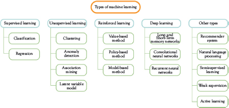
Figure 2.1 Types of machine learning

Supervised Learning

In supervised learning, algorithms learn by example with some form of supervision. It’s almost like having a teacher supervising students, except that the students are algorithms in this case.

When you train such an algorithm, you provide training data consisting of inputs paired with the correct outputs. The machine will analyze the data in the training phase, looking for patterns that align with the desired outputs. So, you give the computer a bunch of photos of vegetables, and you tell it what each vegetable is. The computer analyzes this data to determine the pattern that leads to the correct conclusion. It will determine that an eggplant is oblong and dark purple, whereas a tomato is round and red.

Subsequently, after training has been completed, you can feed that algorithm new inputs, and it will classify the new data based on the training data it received. Therefore, it will classify oblong, dark purple objects as eggplants and round, red items as tomatoes.

The role of the supervisor is to correct the algorithm every time it makes a mistake. However, since the algorithm is constantly learning, it will eventually get to the point where it no longer makes mistakes.

It is, by far, the most popular flavor of ML. It is the primary technology used in task automation.

Supervised learning can be split into two categories: classification and regression.

Classification Models

Classification requires the algorithm to be provided with data that has been assigned to categories. The algorithm then takes inputs and assigns the categories based on the provided training data, like our previous example.

In real-world applications, the simplest example would be categorizing e-mails as spam or not spam, which is a binary classification problem.

The way it works is that the algorithm is provided with e-mails that are spam and e-mails that are not spam. It looks for the common features among each category. It will then use these patterns to classify unseen e-mails as either spam or not spam. As you already know, it doesn’t always work right. However, every time you tell it that it’s made a mistake, the algorithm learns. If you think about it, a decade ago, spam algorithms were wrong far more frequently than they are now. This is because every time someone marks an e-mail as not spam or vice versa, the algorithm learns. Considering that hundreds of millions of people use the same e-mail system (Gmail, for example), that’s a lot of data for the algorithm to learn from.

Classification models can be used for other things, such as whether the value of a stock or commodity will rise or fall. They can also include more categories, so they don’t have to be binary. For example, if you want to figure out who will win a talent competition with multiple contestants.

Regression Models

Regression, on the other hand, is a predictive statistical process. In this case, the algorithm tries to determine important relationships between dependent and independent variables. The goal is for the algorithm to be able to forecast actual numbers, such as sales and income.

In other words, instead of trying to figure out if the value of a commodity will rise or fall, we want to figure out what the price will be in seven days. Or, instead of determining whether a student will fail or pass a test, we want to know what grade they’ll get. Maybe instead of attempting to figure out if the temperature this winter will be higher or lower, we want to know by how much. While these issues are related, they still represent different problems from their classification versions.

Most fields contain classification and regression problems. However, you must remember that these problems can be solved in multiple ways.

For example, let’s say that you’re a forex trader and you want to predict how the U.S. dollar will perform over the next few weeks so you can profit. You can use a classification model to figure out if it’s going up or down, which will tell you whether to go short or long. However, you could also use a regression model for a more specific prediction, such as what price the EUR/USD will be trading at tomorrow.

In the first case, the situation is a little nebulous. While you might make a profit, the risk is far greater than if you were to use a regression model, which will give you more information to make an effective decision.

The idea is that each approach will give you different types of information that will impact performance and, ergo, the strategy you employ.

Unsupervised Learning

In unsupervised ML, an algorithm will infer patterns from data without the benefit of a targeted or labeled outcome. This type of learning cannot be applied to classification or regression problems because you don’t know what the output might be, making it impossible to train the algorithm like normal.

In other words, unsupervised learning is all about the algorithm learning from data on its own and usually refers to clustering. This means that the training data you provide the algorithm only has inputs, without the desired outputs. Instead, the algorithm clusters the inputs based on the patterns it identifies. The system tries to find significant regularities that it can group. It involves no supervision.

With no guidance, this approach to ML can be challenging because the problems tend to be poorly defined. Unsupervised learning is effective, though, in helping to determine the data’s underlying structure. Also, human interpretation is generally necessary, at the very least close to the end of the pipeline.

Unsupervised learning can discover patterns you wouldn’t have otherwise known about. However, the reality is that it’s not as effective as supervised learning. Another factor that makes supervised learning more applicable to practical problems is that, with unsupervised learning, you have no way of figuring out the accuracy of the results.

Unsupervised learning is generally best used when you don’t have any information related to the desired outcome. One such example would be determining the target market of a completely new product. However, if you want to know more about your existing target market, then you’re better off using supervised learning.

That doesn’t mean unsupervised learning doesn’t have its place. Some ways you can apply unsupervised learning are for clustering, anomaly detection, association mining, and latent variable models.

Clustering

With clustering, you can categorize the data into groups based on their similarity. It’s not an approach that’s widely used for applications such as customer segmentation, though, because it tends to overestimate how similar the groups are and doesn’t see the data points as separate entities.

The biggest issue is that these types of problems are generally not well defined. For example, if you give an algorithm a series of images of various animals, the resulting clustering might not be relevant to your needs.

These images can be clustered in several ways, such as by color, type of animal, or habitat. None of these approaches are technically wrong, but some might be more useful than others.

The effectiveness of the result depends mainly on what your goal is. Therefore, it’s important to have a well-defined goal and to experiment until you get it right. The good news is that if you test various algorithms, in the end, you will find one that works.

Anomaly Detection

Anomaly detection is useful for finding unusual information in your data. If something is unusual or anomalous in the data set, these algorithms will find it.

These algorithms have a wide range of realworld applications, especially for things like spotting fraudulent transactions. They can also be used to spot spikes in sales of various products but are just as helpful in detecting hackers.

Association Mining

Association mining is often used for basket analysis because it effectively identifies items that appear together frequently in your data. It’s often used to help determine correlations in transactional, sales, and even medical data.

Latent Variable Models

Latent variable models are used to make the data easier to analyze and come in during the preprocessing phase. These models are effective for doing things such as lowering the number of features in a set of data, also known as dimensionality reduction, or even splitting the data up into multiple components.

With dimensionality reduction, the goal is to group together large numbers of variables into a lower number of factors, making the data easier to interpret. One of the most widely used techniques is factor analysis.

An example is the Big Five Personality Inventory, which was developed by gathering data from a large number of people and applying factor analysis to group the answers into five overall factors. Based on the Big Five personality theory, our personalities can be categorized as:

• Extraversion

• Agreeableness

• Conscientiousness

• Neuroticism

• Openness to experience

However, each of these major factors is made up of a wide range of variables. For example, an extroverted personality is characterized by friendliness, cheerfulness, assertiveness, and much more.

Dimensionality reduction can be applied to many other problems, including user demographics and customer data.

Reinforcement Learning

Many experts believe reinforcement learning to be one of the keys to unlocking real AI because of the vast potential it holds. Moreover, it is growing at an accelerated pace and producing a wide range of algorithms for various applications.

Reinforcement learning is based on a punishment/reward system. It’s a little like training your pet pooch. If you want to teach Fido to sit on command, you’ll give him the command, show him what you want, and reward him with a treat. For a while, you continue to reward him every time he gets it right to reinforce the behavior.

When Fido doesn’t listen to you, you usually have to repeat what you want until he does it and then reward him. Not receiving a reward is generally “punishment” enough for him to get that he’s done wrong.

With an algorithm, things work slightly differently, but in essence, they are the same. For example, let’s consider a robot learning to walk. If the step it takes is too long, it loses its balance and tips over. That’s the punishment. So, it will keep changing the length of its step until it can move without falling over, which is the reward.

Or consider the same robot attempting to navigate a maze. Things are a little more complex here because it’s not just an immediate solution. In the previous example, adjusting the length of the step will yield immediate results. With a maze, the first few steps might be right, until it reaches a dead-end and has to backtrack until it finds open space.

You might be wondering what the point is. Well, consider some real-world applications. Reinforcement learning is used for such things as driverless cars, robot vacuum cleaners, and more. Without reinforcement learning, your vacuum cleaner would keep slamming into the same obstacle instead of backing up to move around it.

Reinforcement learning is the closest thing to learning like a human. Consider that any skill you learn and develop is based on experience. Therefore, the more you practice, the better you get. However, it all boils down to reward/punishment. You’ve learned by discovering what works and what doesn’t.

Consider chess. The more you play, the better you get. That’s because you amass more and more experience on what works and what doesn’t in different situations.

Reinforcement learning for machines works much the same way, which is why so many consider it to have so much potential. It allows for the resolution of very complex problems in a variety of environments.

Deep Learning

Deep learning studies neural networks that have multiple layers, also known as deep neural networks. A neural network is made up of neurons and the pathways that connect them, a bit like a connect-the-dots picture. The human brain is the most powerful computer that exists, so it makes sense for us to model artificial computers on something that already works so well.

In deep learning, artificial neural networks are used to help machines learn more quickly, more effectively, and at far greater volumes. It has been used to solve various problems that were believed to be unsolvable, such as natural language processing (NLP), speech recognition, and computer vision.

At a very basic level, the way it works is that the input is generated from observation, which is then added to a layer. That layer generates an output, which becomes the input for the following layers until you get to the final output.

For example, when you look at a picture of an eggplant, you know it’s an eggplant. But how do you know it’s an eggplant and not an airplane or a basketball?

Your eyes see a specific shape and a specific color, and, based on experience, it translates those inputs into an abstract concept you understand. All this information is filtered from your eyes through multiple layers until it becomes an eggplant rather than an airplane.

Software applications such as Siri, Cortana, or Dragon Naturally Speaking can all understand you because of deep learning. It’s also what allows these applications to learn and improve the more they interact with you.

This also applies to image or song recognition. Want to find out what a specific song is? Just get your app to listen to it, and it will be able to identify it. Likewise, want to find a particular item you can see in the real world? Take a photo of it, and the app will find it for you online.

Deep learning can also be used to generate language. OpenAI’s GPT-3 is a very impressive model that can create articles so realistic that it is practically impossible to figure out a machine writes them.

Another application for deep learning is that it has given computers the ability to identify different subjects in an image, such as being able to tell that chickens, horses, cats, and humans are different things.

It’s also being used in things like graphic design with plugins and apps that can remove backgrounds from photos while maintaining the full integrity of the subject. If you’ve ever tried to remove a background, you know how difficult it can be.

If it’s not something you’ve attempted, then trust us when we say that, before deep learning enabled the creation of these apps, you needed a lot of time and patience. Even then, you still weren’t guaranteed to get a result as good as these apps can offer in a fraction of the time.

It’s a bit like the difference between hand painting one of those eggs with highly complex designs and painting your bedroom wall with a spray gun.

In conclusion, deep learning has allowed us to achieve some incredible things with machines and will continue to do so. Some believe that it might lead us to true AI, whereas others say that progress has plateaued. The big question for AI researchers is: what comes after deep learning? Only time will tell.

Other Types of ML

Quite a few other types of ML exist, including recommender systems, NLP, active learning, semisupervised learning, and weak supervision.

Recommender systems are designed to predict user interest and make recommendations accordingly. These are some of the most powerful ML systems used by retailers online to boost sales (Rodriguez 2018).

Consider Amazon, which has an excellent recommender system. Every time you log in, Amazon will recommend products or books they think you might like based on previous purchases and visits.

Spotify or Netflix use similar data to make recommendations in terms of the content you might enjoy. For example, if you watch a lot of action movies and crime dramas, then Netflix will recommend similar films and TV shows.

In ML, Natural Language Processing and text analytics involve the use of algorithms and AI to understand text, which can range from Facebook comments and online reviews to e-mails and regulatory documents (Barba 2020).

Active learning refers to the process of prioritizing data that must be labeled, so it has the highest impact on training a supervised model (Solaguren-Beascoa 2020).

Semisupervised learning combines supervised and unsupervised ML methods so that an algorithm learns from data sets that include labeled and unlabeled data (“Semi-Supervised Machine Learning” n.d.).

Weak supervision or weakly supervised learning comprises a variety of approaches, including:

• Inexact supervision, where the training data is provided with only coarse-grained labels;

• Incomplete supervision that features data sets with only one subset that has labels;

• Inaccurate supervision, where the labels aren’t always ground truth (Zhou 2018).

For Decision Makers: How to Use Machine Learning

Machine learning really shines in cases where automation or prediction are needed. Irrespective of the actual form of ML being used in most cases, it is applied to the following cases:

1. Humans are performing a repetitive task, which also allows them to label data. The labeled data can then be used to train a ML model to replace the human. The most prominent example of this is computer vision and applications such as face recognition or recognizing certain entities in a photo (e.g., humans vs animals).

2. Predicting something about the future or an unknown quantity: credit scoring, spam detection, forecasting, customer churn all are viable applications of ML.

Understanding when and how to apply ML is a skill that takes a long time to master. However, a decision maker can just use the aforementioned heuristics to get a feeling of when they could use it. What is more important from a decision maker’s perspective is making sure that there is a data strategy in place that can facilitate the use of ML. This is covered in the next chapter.

A Brief Intro to Statistics for the Decision Maker

Statistics is one of the core fields of data science. It was the first discipline to deal with data collection and analysis in a systematic way. In this section we will provide a brief overview of that area, as it can help us better understand the domain of data science.

Statistics is the study of how to collect, organize, analyze, and interpret numerical information and data. It encompasses both the science of uncertainty and the technology of extracting information from data.

It is a vital tool for any data scientist and is used to help us make decisions. This field employs a variety of methodologies that enable data scientists to do a variety of things, including:

• Design experiments and interpret results to improve product decision making;

• Develop models to predict signals;

• Mold data into insights;

• Understand a wide range of variables, including engagement, conversions, retention, leads, and more;

• Make intelligent estimations;

• Use data to tell the story.

From a decision maker’s perspective, statistics is important to understand, and also to get a good understanding of how they fit into the whole narrative of data science. While the discipline of statistics cannot be considered an emerging field (since it has been around for more than 200 years), it has found new uses in the era of big data.

Many data science applications, which could be considered emerging tech, are based on simple applications of statistics. Therefore, getting a good understanding of the basic uses of statistics can help put things into perspective as to how technologies and methodologies evolve and adapt as technology advances.

A Little History About Statistics

Statistics is a branch of mathematics dating back to approximately the 18th century. It was humanity’s first attempt to analyze data systematically and is at the base of modern data analysis. It led to the development of summary statistics, regression classification, significant testing, forecasting, and more. Some prominent individuals in this field include Ronald Fisher, Karl Pearson (and his son Egon Pearson), and Jerzy Neyman.

Statistics is different from other data analysis fields because it focuses more on the theoretical soundness of the models and has traditionally dealt with smaller samples. This is mainly due to historical reasons because data had to be collected in person until relatively recently. It’s only since the advent of the Internet that we can collect data remotely, allowing for much larger sample sizes.

As you can imagine, collecting data in person was not only expensive but also time-consuming, which meant that small sample sizes were the norm. Furthermore, until computers became part of our lives, calculations had to be done manually. While the results were extrapolated to the entire population using a margin of error, those calculations still took time. Today, solving a model might take seconds, but in the 18th century, it would’ve taken days or weeks.

There’s also a different mentality when it comes to statistics. As this field is rooted in math, it is very strict on model assumptions and development. These assumptions must be validated and verified before you can do anything else. On the other hand, in ML, the goal is to achieve the objective and ask questions later.

One crucial difference between ML and statistics, for example, is that ML has led to impressive performance, even though statistics is far more transparent and has a higher degree of interpretability. The thing is that the high-level performance ML offers means that we’ve been able to achieve things that were previously thought impossible.

While some statisticians are completely against ML because of the reduced level of transparency and lack of theory, the fact is that statistics and ML work hand-in-hand. They are also both tools the data scientist can and should use depending on the situation. In other words, if you want interpretability, then you should turn to statistics. On the other hand, if you’re looking for performance and predictive power, then ML is the way to go.

A Short Intro to Statistics

Statistics can be split into two branches: descriptive and inferential statistics.

Descriptive statistics is what most people consider statistics to be. It involves collecting data, using summary metrics such as the name and data visualization.

On the other hand, inferential statistics is what most people in the field consider to be statistics. It involves more advanced concepts such as sampling and inferring values of the population parameters.

Descriptive Statistics

Descriptive statistics involves organizing, summarizing, and presenting data so everyone can understand and make use of it. To do this, there are two sets of methods, namely numerical methods to describe data and graphical methods for data presentation (“Understanding Descriptive and Inferential Statistics | Laerd Statistics” n.d.).

Numerical methods encompass metrics not only for data location, such as the mean, median, and mode but also measures of data variability, such as variance and standard deviation.

Graphical methods for data representation include bar charts, histograms, pie charts, and more.

Many analytics products in the market, such as Tableaux or other dashboards, are usually focused on descriptive statistics. While descriptive statistics are simple, they can be very effective and easily understood by anyone.

Inferential Statistics

Inferential statistics represents the majority of the field because that’s where the work is really done, while descriptive statistics represents a tiny fraction.

Inferential statistics comprises a group of methods you can use to draw conclusions or inferences about the traits of a whole population based on sample data.

In essence, inferential statistics allows you to quantify uncertainty. So, for example, let’s say that you want to figure out something about a group of people. It could be something like the average age of the population.

If you were dealing with a small population, say maybe a few hundred people, then you could measure everyone’s age and calculate the average. However, when you try to do that for an entire country, for example, that might have a population of 20 million people, it will be practically impossible. Well, at least unfeasible from a cost and effort viewpoint.

So, if studying every individual is impractical, there must be an alternative. That’s where inferential statistics comes in. It involves taking a sample of the population you are attempting to study and expressing uncertainty through probability distribution. You’re essentially turning uncertainty into a quantifiable metric, which then allows you to run calculations. That is what permits statistical modeling and hypothesis testing.

What you do is take a sample of a thousand people, which covers as wide a demographic as possible and then extrapolate their average age to the entire population of 20 million. While demographic conformity is not absolutely necessary, it does lead to more accurate results.

For example, consider deaths caused by the coronavirus. There were many conversations over the first few months of the pandemic about the actual mortality rate of the disease. Many disagreements arose between statisticians. At least some of those deaths attributed to COVID-19 were caused by other conditions. Still, at the same time, some covid-related deaths, especially before tests became available, were attributed to other illnesses. This is a classic problem of inferential statistics: trying to decipher the value of an underlying variable, given a sample.

Another interesting inferential issue around COVID-19-related deaths is related to definitions and attribution. Let’s say someone had severe underlying conditions and would probably die within the next month. If this person died and then tested positive for COVID-19, was the illness the cause of death or the underlying conditions?

The topic of attribution raises more of a philosophical discussion and is encountered in many health-related discussions. For example, who is the true culprit of the obesity epidemic? The companies selling unhealthy food, the advertisers, or the people buying it? While many people will have strong opinions on the subject, it is difficult to attribute this phenomenon to a single factor completely. This is where inferential statistics can help provide more clarity by quantifying each factors’ contribution.

The Benefits of Statistics

All this might sound very interesting, but you’re probably wondering how statistics can help you in business as a decision maker.

First, you’re probably already using descriptive statistics in some shape or form. Profit and loss forecasts are just one example of using statistics in a business setting.

Inferential statistics, on the other hand, can be used to answer specific questions regarding the importance of a variable. It can also answer questions about differences in population.

The main things you’ll be using inferential statistics for are hypothesis testing and statistical modeling. While forecasting is another beneficial area, it is somewhat more technical, and it can often be achieved using ML more easily than through statistics.

Hypothesis testing is generally used for finding out the value of a population parameter or making comparisons.

Working out the value of a population basically means that you are looking to determine the specific value, such as average height, average income, and average age. Comparisons involve analyzing the differences and/or similarities among parameters. One example would be exploring differences based on gender. So, you would look at whether men earn more or less money in a specific job than women.

In business, especially online, you might have already heard of A/B testing, which is a form of comparison. So, when you test two calls-to-action against each other to determine which generates the highest conversion rate, you are conducting a comparison-based hypothesis test.

Statistical modeling is what you use when you want to figure out if one variable affects another.

So, let’s say you’ve conducted your comparison-based hypothesis test on your calls-to-action to determine which is more effective at achieving conversions. You’ve established which one is more successful, but you also want to learn what other variables could be affecting your conversion rate. To do so, you would use statistical modeling.

Essentially, you plug in your variables into the model and may discover that everything. from the button’s position on the page and the color of the text to the headline and content, affects conversion rates. You can also determine to what degree these variables affect conversion rates. For example, you might find that the headline and call-to-action play only a small part in why people are converting and that the main draw is the offer itself.

Applications of Statistics in Business and Economics

In today’s digital world, we have vast amounts of statistical data available to us at our fingertips. The most effective business leaders and decision makers are aware of the value of this data and can use it effectively. Here are some of the applications of statistics in business:

Accounting

Accounting companies often use statistical sampling methods when they conduct audits for clients. For example, let’s say that an accounting company wants to figure out if the accounts receivable on the client’s balance sheet accurately represents the total amount of accounts receivable (Dilip n.d.).

Large corporations often have significant numbers of individual accounts receivable, which makes it far too time-consuming and expensive to validate each entry. Thus, the audit team will often select a sample of those accounts and, after reviewing and validating them, the auditors will conclude whether the amount on the balance sheet is accurate or not.

Finance

Financial analysis involves the use of a lot of statistical information to help investors make decisions. For example, Forex trading relies on the analysis of financial data, including historical price movement, a country’s economic data, and much more. It also involves using a wide range of indicators that are calculated using statistical information, such as the moving average.

The same applies to stocks, where investors make decisions on which stock to invest in based on variables such as price/earnings ratios and dividend yields. Some might even conduct a comparison between the market average and the results of an individual stock.

Marketing

Statistics is also highly useful in marketing. Electronic scanners at retail checkout counters collect data for various marketing research applications. AC Nielsen, an information supplier, purchases this data from grocery stores, then processes it and sells statistical summaries to manufacturers and distributors, among others.

Companies will spend a lot of money to obtain this kind of data because it can be used to determine production necessities and even assist in developing new products.

Production

Quality control is an essential application of statistics in manufacturing. Various statistical quality control charts are used to monitor the output of the manufacturing process, such as an x-bar chart, which can be used to monitor average output.

For example, let’s say that a machine fills containers with 1.5 ounces of cream. Sporadically, an employee will select a sample of containers and calculate the average number of ounces in the sample. This average value is then plotted on an x-bar chart.

A plotted value above the upper control limit indicates that the machine is overfilling the containers, whereas a plotted value below the lower control limit indicates underfilling. The process continues as long as the plotted value falls between the upper and lower control limits. Otherwise, adjustments are made to ensure the average is where it should be.

Economics

Economists frequently predict the future of the economy or certain aspects of it. They use a variety of statistical information to make these predictions, such as forecasting GDP, inflation rates, and more. However, these predictions are often made using ML.

Information Systems

Information systems administrators handle the daily operations of the company’s computer networks. They use various statistical information to assess performance and make adjustments to ensure that the system is functioning optimally.

The Pitfalls of Statistics

One of the biggest problems with statistics is that people tend to trust them blindly simply because they appear to be facts. After all, when someone presents you with information, and it’s backed by what looks like accurate data in the form of numbers, ratios, percentages, graphs, charts, and so on, you’re far more likely to believe what you’re being told.

However, it is very easy to use statistics to lie to people. While it’s not always a matter of bad intentions, even human error can lead to skewed results, which can cause problems.

Therefore, it’s essential that you understand how statistics can be used to distort facts. This way, you will be more aware and less likely to make poor decisions because you’ve been misled.

Here are some of the ways in which you can be lied to using statistics:

Lying Using Charts

One way statistics can be used to mislead an audience is by lying to people using charts that contain spurious correlations. They seem to make sense at first glance but have no connection one to another.

For example, here is one chart that correlates the divorce rate in Maine with the per capita consumption of margarine (Figure 2.2).

Here’s another chart that attempts to correlate worldwide noncommercial space launches with sociology doctorates awarded in the United States (Figure 2.3). Now, these might seem like interesting statistics and, separately, they certainly are. However, when you try to establish a correlation between these facts, it’s a bit ridiculous.

For example, the first chart seems to imply that as divorce rates decline in Maine, so too does the consumption of margarine. Some enterprising individuals might attempt to convince you that margarine has affected the divorce rate, and the less margarine people eat, the less likely they are to get a divorce.

The second chart seems to imply that an increase in sociology doctorates has led to a rise in the number of worldwide noncommercial space launches. Now, you might scoff and say that it’s quite obvious there are no correlations between these variables. After all, how can the number of sociology doctorates awarded in the United States affect space launches? However, what happens is that people use variables that might seem to have a tangential connection to each other to attempt to convince you that a spurious correlation is fact.

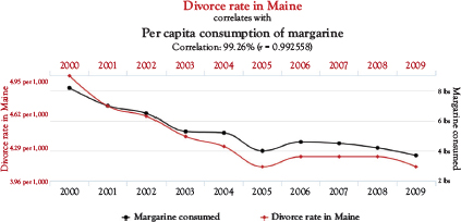
Figure 2.2 Divorce rate in Maine

Sources: National vital statistics reports and U.S. department of agriculture

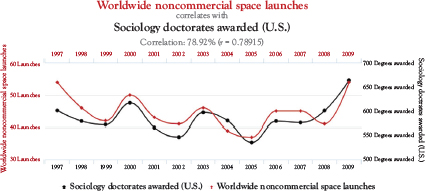
Figure 2.3 Worldwide noncommercial space launches

Source: Federal aviation administration and national science foundation

A spurious correlation means that someone is trying to correlate two variables that don’t really have an underlying theory that holds up to scrutiny. They are simply comparing two variables that aren’t connected. Furthermore, it’s important to remember that correlation doesn’t necessarily imply causation.

For example, the consumption of margarine is in no way related to the number of divorces in Maine. After all, it’s not like a spread can have such an impact on people’s relationships. You might go so far as to say that an argument over margarine led to a divorce. However, if people are arguing over margarine so much that they end up divorcing, there are many other underlying issues, and margarine is only an excuse rather than a cause.

However, if we were to attempt to correlate the consumption of margarine and income in the margarine industry, then the correlation would make sense because the two are connected.

In some charts, people can be tricked even more because things like reversing the X- and Y-axis can lead to mistaken conclusions. For example, suppose the numbers along the X-axis decrease while those on the Y-axis increase. In that case, this will lead to an erroneous visual representation, which is another way to attempt to force a correlation.

So, just remember that even if there might seem to be a significant correlation between two variables, that doesn’t actually mean there is a relationship between the two.

Another way you can be lied to with charts is by using different types of scales in the same chart. For example, you can use different scales to make items seem as if they’re closer to each other.

Another way to lie is to change the scale. If you close in on the scale, a variable’s evolution might seem choppy. However, when you zoom out, it looks far more stable.

For example, if you take a snapshot of last year’s performance of the Dow Jones industrial index (simply google “Dow Jones chart”) you will see that growth has stalled (Figure 2.4). But if you look at a multidecade chart, you will see that the index has been rising over the long run (Figure 2.5). An analyst who focuses on recent developments might get worried, while someone focused more on the long run can be reassured that the economy will simply keep growing. Graph interpretation can be quite subjective at times, and this is why a decision maker must always be skeptical and critical of any graph interpretations.

Embellishing With Descriptive Statistics

Descriptive statistics can also be used to mislead people, and one way to do so quite easily is through measures of centrality and summary metrics.

You have three main measures of centrality: the median, the mode, and the mean.

The mean represents the average of a set of numbers, which is basically where you add all the numbers together and divide the result by the number of variables you added together. The median is the central value in a list of numbers, and the mode is the value that shows up most frequently in a list.

If a distribution is symmetrical, these three values will fall on the same point. However, if the distribution is positively skewed, the mean will be lighter than the median, and the median will be lighter than the mode. If the distribution is negatively skewed, then the opposite happens.

It’s important to note this because most distributions in life aren’t symmetrical. For example, let’s say that a company pays its CEO $300,000 per year, while the rest of the 10 employees earn $50,000 per year each.

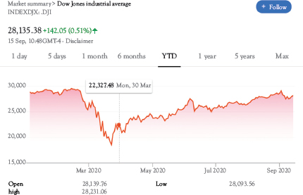
Figure 2.4 Dow Jones industrial index for 2020

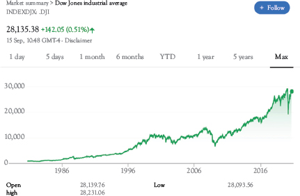
Figure 2.5 Dow Jones industrial index long-term trend

Depending on what you want to achieve, you can present different numbers. In this case, the median might be $50,000 per year, but the mean is $72,000 per year.

A company could advertise the mean figure, which would make people think that that’s what they could earn, but the company is unwilling to pay more than $50,000 per year for anybody other than the CEO.

This way, they could trick potential employees into accepting a job because they believe they will eventually earn $72,000, when in fact, they’ll never receive more than $50,000. It might seem underhanded—it is, in case you were wondering—but not as unusual as you might think.

Sampling Biases. Sampling biases can also lead to less than accurate data that can cause problems in the decision-making process. While there are quite a few different sampling biases, we will be looking at five: the selection bias, the area bias, the self-selection bias, the leading question bias, and social desirability bias, as they are the most common in business.

Two very famous cases of sampling bias are the forecasting of the Brexit vote in Britain and the 2016 presidential election in the United States. The forecasters in both cases got it completely wrong, because of bias that got introduced into the sample and completely invalidated most statistical models that were used (Kampakis 2016).

Selection Bias. The selection bias is the most significant. In fact, the other types of bias can actually be seen as related or even as subcategories of selection bias.

Selection bias occurs when the sample being used is not representative of the whole. Something is going on that ensures the subjects or items in the sample are special somehow, while other subjects are left out.

One interesting example of selection bias is the attempt of the U.S. government to increase the survival rate of U.S. aircraft during the Second World War.

The initial attempt was conducted after investigators analyzed planes that had survived. The recommendation was to add more armor to the areas that had received the most amount of damage. When the armor was mounted, instead of leading to a higher rate of survivability, the exact opposite happened. The extra armor made the planes heavier, slower, and far less agile, making it easier for the enemy to destroy them. Furthermore, the aircraft that survived still had significant amounts of damage in the same areas.

The government turned to Abraham Wald, who was a statistician. He realized that selection bias was taking place. In other words, instead of looking at what was important, the investigators made their decisions based on planes that had survived the damage they received. That’s when Wald concluded that the areas that required protection were actually the areas that were sensitive and hadn’t been damaged. Once those areas were reinforced, survivability increased (Mangel and Samaniego 1984).

This is an interesting way that you can use statistics without even conducting any significant analysis. Wald had to understand that selection bias was taking place, which allowed them to fix the problem.

Area Bias. Area bias refers to attempting to generalize results from one area to another. This poses many problems, especially when you’re trying to cross cultures.

For example, if you conduct marketing research in the United States, and you attempt to apply the results to another area, such as the Middle East, you’re going to have a big surprise. The cultural, financial, lingual, and many other differences will have a significant impact, basically making those results null and void.

Self-Selection Bias. Self-selection bias refers to the increased likelihood of a person deciding to participate in a study because of traits they already have.

For example, if you conduct a study on using makeup, you are more likely to get people participating in the survey who use makeup frequently than those who don’t at all or do so rarely.

The problem is that this leads to a nonrepresentative sample. Of course, this depends on what you’re attempting to achieve. However, if you want the sample to be truly representative, you need to talk to people who use makeup and who don’t use makeup or use it rarely.

Leading Questions Bias. A very easy way to get the answers you want rather than the truth is to use leading questions in your questionnaires. For example, if you ask someone if they believe teachers aren’t paid enough and the answers you provide them are:

(a) Yes, they should earn more;

(b) No, they should not earn more;

(c) No opinion.

Most people will say A; teachers should definitely be paid more. This is because people want to be nice and provide what seem like socially acceptable answers. Plus, the way the question was phrased only really gives them one option.

Social Desirability Bias. Social desirability bias occurs when people want to paint themselves in a better light, which is almost always. So, if you pose questions about social desirability issues, your data will be skewed because nobody wants to admit they don’t fall in line with societal expectations. So, for example, if you ask someone how frequently they donate to charity, or how often they recycle, or how much food they throw away, you are unlikely to receive accurate answers.

If someone tells you that they only throw out 3 percent of the food they buy, they are probably not telling the truth since throwing away food is not exactly considered socially acceptable as it’s a massive waste. So, they will provide an answer they feel is more socially acceptable instead of the truth.

Lying With Inferential Statistics

Some believe that it’s impossible to lie with inferential statistics. Unfortunately, that’s not exactly accurate. It might be challenging to lie with inferential statistics, but it can still be done.

This takes place a lot in research. When testing a hypothesis, you’ll get a p-value. This value needs to be below a certain threshold for the tests to have statistical significance. Generally speaking, this threshold is 0.05.

A theory says that a significant number of research papers have p-values that are unusually close to 0.05. In other words, the results of these papers seem significant, but only by a tiny margin, because the value of p is just below 0.05, allowing them to meet the condition of the statistical significance.

The theory in question says that this is being done on purpose. Academia is a very competitive environment, and people have to publish papers, or they’ll end up without a job. So, people are basically under pressure to make the results look as if they are statistically significant. One way to achieve this is by conducting multiple experiments until you get the results you want.

Another way to do this is by massaging the data. However, in other cases, you can find research where the results are significant, but this is only because the model assumptions aren’t being met and not because the researcher intended to deceive.

Case Studies and Examples

Here are some examples where data science can make a significant impact on business.

Preventive Maintenance Becomes Predictive Maintenance

Preventive maintenance is a key aspect of business for many firms across a wide range of industries because of the reduction of unplanned down-time. The latter can negatively affect the bottom line, which is why preventive maintenance is so valuable.

Like with any other aspect of business, improving maintenance efficiency is a big priority for many firms, especially those that rely on a lot of expensive machinery. Companies operating in industries such as manufacturing, shipping, oil and gas, rail, and freight can all benefit.

The goal of regular maintenance is to minimize failures, maximize the life of a machine, and ensure optimal performance and efficient operation.

The most common approach is for firms to use a maintenance schedule based on recommendations made by the manufacturer of the equipment or vehicles. It’s just like with your car, where the manufacturer recommends you change the oil after 10,000 miles, for example.

This isn’t a bad approach at all. It’s certainly better than guessing or waiting for something to break down. However, it isn’t ideal because failures still happen. The fact is that no one can plan for every situation and predict every issue.

For example, a manufacturer might recommend that you change fuel filters every 5,000 hours of operation, but that’s in ideal operating conditions. If the diesel hasn’t been the best quality or the machine is operating in very dusty or sandy conditions, the change will need to come sooner unless you want a lot of other problems to occur.

Avoiding unplanned downtime due to failures and breakdowns is essential because this downtime can be very expensive. It leads to a significant loss of revenue through lost output and reduced productivity.

The better alternative is planned downtime because you can plan to conduct maintenance at a time when the machine being inoperable will cause the least amount of problems. The key is figuring out when that is.

Many firms are turning to data and predictive analytics to solve their issues with maintenance scheduling (Kampakis 2020a).

In manufacturing, for example, the sensors on a production line can collect almost any information you need. You can then store and analyze the data. Algorithms can then use the data to determine when a failure might occur. This process is referred to as predictive maintenance.

The predictive maintenance algorithms being used at the moment are usually based on ML, so their accuracy improves as they get better at identifying situations when failures are possible.

Furthermore, the whole process can be automated, which means that predictive analytics can work out when maintenance is necessary to avoid failure. It can also determine the best time for maintenance to occur to ensure it is the least disruptive, based on a variety of factors such as demand.

Predictive maintenance offers significant boosts in productivity, improves customer service, reduces costs, and improves profits. As Google trends show, it has become very popular and will continue to increase in popularity as more firms understand the benefits.

Using AI and Data Science to Fight COVID-19

Owing to the novel coronavirus dubbed COVID-19, the world is facing a crisis that no one thought could occur in the modern world. At the time of this writing, the death toll has almost reached one million on a global scale with a total of 31.4 million cases of infection, and the crisis is still ongoing, with many experts warning of a second wave of mass infections.

Many organizations have turned to AI and data science to help in this time of crisis (Kampakis 2020b). The White House and the Allen Institute for AI have released a database of 29,000 research articles on the coronavirus family. These articles have been modified to ensure they are machine-readable by NLP libraries.

Using AI, researchers hope they will be able to generate new insights from all the work that’s already been done into understanding this virus family.

The data set has also been put up as a Kaggle challenge to take advantage of crowdsourcing to come up with new insights and possible solutions.

AI can also assist in detecting people who are very vulnerable to infection and developing severe complications from the virus. Medical Home Network uses such a system to first address those patients who are most in need of medical care.

AI can also help to create vaccines. A team from Australia’s Flinders University designed an AI that managed to develop a drug on its own for the first time. While the technology is still in its infancy and not much help fighting COVID-19, it could be vital for a future pandemic.

AI can also help to reduce the strain on health care networks, with chatbots replacing doctors to answer simple questions. For example, Ask-Sophie helps patients determine whether they have a common cold or COVID-19 (“Check Your Symptoms | Medicare” n.d.).

Traditional predictive analytics can also help forecast the future. Researchers in Israel, for example, are relying on AI to predict when the next breakout might occur, so they are in a better position to prevent it. The Israelis don’t have a large number of tests available, so they need to be careful how they use them. They are, therefore, handing out questionnaires daily and relying on data science to work out which clusters of people could be infected.

Hiring the Right Person

As it has become clear by now, data science is a big and convoluted field, primarily because it is an aggregation of different scientific disciplines. This means that there are many different types of data scientists, and hiring one can be a fairly complicated process, as backgrounds can vary. A ML specialist might have a very different skillset from a pure statistician. We are looking into the topic of hiring and managing data scientists in Chapter 4 later on.