THE CCNP ENCOR EXAM OBJECTIVES COVERED IN THIS CHAPTER INCLUDE THE FOLLOWING:
Domain 1.0: Architecture
✓ 1.1 Explain the different design principles used in an enterprise network
Domain 3.0: Infrastructure
✓ 3.1 Layer 2
✓ 3.4 IP Services
Ultimately, the performance and flexibility of any network hinges on the physical topology—that is, the physical connectivity between devices. After that, every subsequent decision is a logical configuration decision that depends in some way on the physical topology. In other words, the physical topology determines the path traffic can take, but the logical layer 2 topology determines what path the traffic will take. In this chapter, we'll look at how different layer 2 designs influence traffic patterns, which in turn influence bandwidth and reliability. We'll then turn to EtherChannels, which can help you make efficient use of your physical links as well as make your network resilient to link failures. Finally, we'll cover three first-hop redundancy protocols that let you create a highly available default gateway for hosts in a subnet.
Physical Network Architectures
The physical design is the first important decision you'll make when designing or revising a network. Recall from Chapter 1, “Networking Fundamentals,” that everything else rests on the physical design: the Data Link protocols you can use, the number of subnets you can support, and the size of those subnets. It also goes without saying that the physical design influences bandwidth and reliability. More physical connections can give you more bandwidth and redundancy. However, there's another consideration that's often overlooked: traffic patterns. The path traffic takes in a network has a profound influence on throughput and reliability. Every network design should take into account, first and foremost, the expected traffic patterns.
The physical topology of a network is its least flexible and most unforgiving aspect. If you botch a configuration, you can fix it with a few keystrokes. If you botch the physical design, it can lead to poor performance and even downtime. A poor physical design can't be fixed with configuration commands. The physical design also determines the network's scalability in terms of the number of devices that can use it and how much data they can push through it.
Good physical network design isn't hard, but the physical design of a network strongly influences its cost, and not everyone can afford to build a dream network right out of the gate. So, in this section you'll learn about two physical architectures: the three-tier architecture, whose strength is scalability, and its more cost-effective but less-scalable relative, the two-tier collapsed core architecture.
Comparing Campus and Data Center Networks
As with many technology buzzwords, the term “enterprise network” gets thrown around a lot without any clear definition. Although there isn't a unanimously accepted definition of the term, we can loosely define an enterprise network as a private network that's under the control of a single organization and that consists of at least one of two type of networks: campus networks and data center networks.
Campus Networks
Enterprise networks include campus locations, a fancy term for where users sit with their end-user devices, such as computers and phones, as well as shared devices such as printers, copy machines, and wireless access points. Typically, a campus location is an office but could be any place where multiple users work, such as a warehouse.
The key feature of a campus network is that it connects users to the network resources that are not on campus—be they applications running in a company data center or web applications on the Internet. The majority of traffic traversing a campus network is not between devices on the campus. Instead, it's mostly client-to-server traffic, also known as North-South traffic.
Data Center Networks
An enterprise network may also include a data center consisting of servers and mass storage devices. Typically, a data center resides in a dedicated facility. The company may own the facility, or they may lease rack space from someone else. Consequently, a key feature of data center networks is that they don't include end-user devices. Instead, users connect to a data center network over a wide area network (WAN) connection such as a private line, Multiprotocol Label Switching (MPLS) layer 3 virtual private network (VPN), or the Internet.
Naturally, data centers have substantial client-server traffic flows. But in a data center network, the bulk of traffic is server-to-server traffic, also known as East-West traffic. East-West traffic includes countless activities, such as
An application server pulling data from a database server
Migration of a virtual machine (VM) from one VM host to another
Data replication from a server to a backup storage device
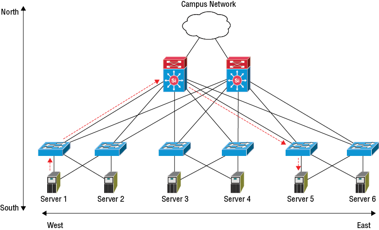
East-West traffic includes a lot of sustained or bandwidth-intensive traffic. Figure 3.1 illustrates the East-West traffic flow typical of data center networks.
The design shown in Figure 3.1 is known as the leaf-and-spine architecture. It's a popular design in data center networks because it provides a predictable number of hops between any two servers. Equal-cost multipath routing (ECMP) can simultaneously use multiple equal paths between servers to increase available bandwidth.
Figure 3.1 East-West traffic flow in a data center network using the leaf-spine design
It's not unusual for a company to have a data center (or in a small company, a data closet) in a campus location, particularly if that location is the company headquarters. Even in this situation, a clear line of delineation must exist between the data center network and the rest of the campus. To put a finer point on it, there shouldn't be a server sitting in someone's office!
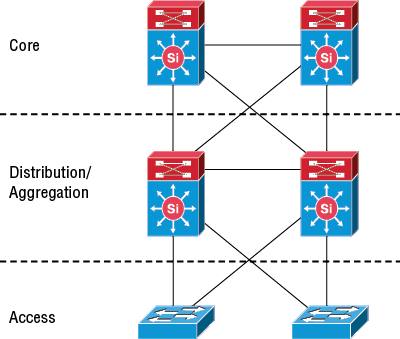
The Three-Tier Architecture
The three-tier architecture has been the standard for enterprise networks for years. It's a modular design that has the advantage of easily scaling to accommodate growth. The three-tier architecture is shown in Figure 3.2 and consists of three layers: core, distribution or aggregation, and access.
Scalability is an area in which the three-tier architecture really shines. The modular approach means costs and configurations are predictable and consistent. The biggest drawback to this architecture is the cost. Unless you need maximum scalability, it's not very cost-effective.
From a physical design perspective, the core layer is the center of the campus or data center network. As such, core switches tend to have a high port density and carry a hefty price tag. Configuration in the core should be minimal to reduce the need for changes and the chance of a misbehaving protocol taking down the entire network. Hence, connections within the core should always be routed. Routed (layer 3) connections provide several key advantages, including load balancing, rapid convergence, and scalability—all necessary features given that the core is the heart of the network. Recalling that large broadcast domains don't scale and provide poor isolation from failures, there shouldn't be a single VLAN that all of your core switches share. Rather, each interswitch link should be a separate broadcast domain, which of course necessitates point-to-point IP routing on each and every link.
Another defining feature of the core is that servers and end-user devices such as computers and phones don't connect directly to core switches. The only devices that connect directly to the core are routers and other switches. But these devices aren't connected willy-nilly. Rather, they're connected in a modular fashion via an access-distribution block.
Access-Distribution Block
The next two layers, the distribution or aggregation and access layers, together form what's called an access-distribution block, or just distribution block for short. The term “block” isn't accidental. Think of an access-distribution block as a building block that can be plugged into the core, allowing the network to be expanded in a modular fashion. Figure 3.3 illustrates two access-distribution blocks connected to the core.
Figure 3.3 Two access-distribution blocks connected to the core
Ideally, each module contains devices that share a similar function. For example, desktops and phones may be in one block, routers in another block, and on-premises servers in yet another block. Notice that if devices in a distribution block need to talk to each other (such as two servers), this architecture makes it possible for them to do so without going through the core. This makes scaling the network by adding more devices straightforward. For example, if you have a block with hundreds of web servers, adding more may simply entail adding more access switches without having to make any connectivity changes to the core. The modular approach also provides isolation within the network. Changes in one block are less likely to affect changes in another block. For example, a switch failure in the desktop block shouldn't affect resources in any other blocks, which also aids in troubleshooting.
Distribution or Aggregation Layer
The distribution layer (sometimes called the aggregation layer) serves two important purposes. First, it provides a reliable and consistent connection to the core while conserving valuable switch port space on the core switches. Notice that in Figure 3.3, the distribution switches have redundant connections to each other and the core switches.
Second, the distribution layer can keep the access-distribution block scalable to accommodate device sprawl. You should take into account the number of additional devices you'll need to connect in the future so that you can avoid having to install and connect additional distribution switches to the core. You therefore want to avoid filling up the ports on your distribution switches with a bunch of end-user devices. Instead, you'll connect those devices to switches in the access layer, which we'll get to in a moment. However, this doesn't mean that you can't connect any other devices to the distribution layer. It's perfectly fine to connect things like servers or storage area network (SAN) devices directly to distribution layer switches. In this case, these devices will generally have redundant connections to the distribution layer.
Depending on the devices you're connecting, you may not even need distribution switches in every block. In its simplest incarnation, the distribution layer may consist of nothing but routers connected directly to the core to provide private WAN or Internet access. In this scenario, the layer is called the WAN aggregation layer.
Because client-server traffic passes through the distribution layer, distribution switches and routers are sometimes used to apply policies such as traffic filtering and access control. Just keep in mind that applying policy at the distribution layer is a matter of preference and not a technical requirement.
Access Layer
In a campus network, the purpose of the access layer is to provide physical connectivity to end-user and shared devices such as printers. Access switches may also offer power-over-Ethernet (PoE) to power phones and wireless access points. Switches in the access layer usually have redundant connections to the distribution layer (although this isn't always the case, as you'll see later).
Ideally, you want to keep complexity as close to the access layer (or edge) as possible. For instance, security features such as port security, dynamic ARP inspection, and DHCP snooping should be implemented close to edge devices. Quality of service (QoS) markings also should be applied at the access layer.
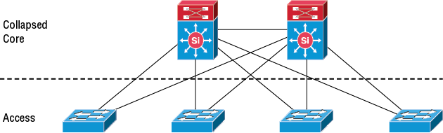
The Two-Tier Collapsed Core: A Cheaper Alternative
The two-tier collapsed core architecture is a simplified (and cheaper) version of the three-tier architecture. It flattens or collapses the distribution layer into the core, leaving a collapsed core. As a result, it sacrifices the modularity and scalability of the three-tier architecture. See Figure 3.4 for an example.
The two-tier collapsed core architecture is more cost effective for networks that will remain at a relatively fixed size. But it does come with some drawbacks. Expanding the network is possible but becomes more complex the more it grows. Adding additional access switches is easy enough. But if the core switches reach capacity so that they can no longer accommodate additional access switches, you'll need to either add additional core switches or redesign a portion of your network using the three-tier architecture.
The lack of modularity also makes change control harder. For example, suppose that you need to add some additional VLANs and trunk ports for servers. Making a change to a collapsed core could bring down the entire network, so that change must be coordinated with everyone who might be affected by it. Contrast this with the three-tier architecture, where the change could be isolated to the distribution switches and thus wouldn't require any coordination with other parts of the network.
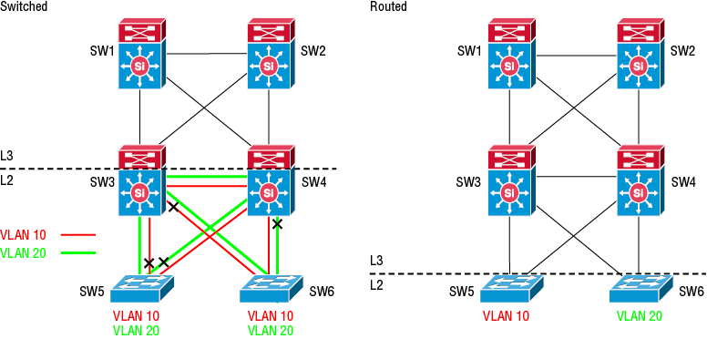
Layer 2 Design
There are really only two types of interswitch connections: switched and routed. As I noted earlier, connections within and to the core should always be routed. But when it comes to the access-distribution block, the choice to use routed or switched interswitch connections is up to you. Essentially, the routed versus switched decision comes down to whether a subnet needs to span multiple access and distribution switches. Referring to Figure 3.5, notice that the main difference between switched and routed is where the layer 2/layer 3 line of demarcation sits. Ultimately, you need to answer the question “Where should IP routing take place?”
Let's start by clarifying the difference between a switched (layer 2) interface and a routed (layer 3) interface. Fundamentally, the difference is in how each handles an incoming Ethernet frame. A switched interface is just what you normally think of as a switchport. Although it doesn't show in the configuration, the interface command to turn an interface into a switched interface is simply switchport. You can verify the switchport status of an interface as follows:
A switchport can be an access port with membership in a single VLAN, or it can be a trunk port that carries traffic for multiple VLANs, as in the preceding example. If a switched interface receives an Ethernet frame, it will either flood the frame or forward it according to its MAC address table. A switched interface cannot have an IP address assigned to it. However, you can create an SVI with membership in a VLAN, and that SVI can have an IP address. When using a switch as a default gateway for a VLAN, you create an SVI and assign it an IP address. You then configure the hosts in that VLAN to use that IP as their default gateway.
A routed interface, on the other hand, effectively terminates a layer 2 connection. Put another way, a routed link is a point-to-point link in its own broadcast domain. If a routed interface receives an Ethernet frame, it checks to see whether the destination MAC address is the same as its interface MAC address. If it's not (as would be the case with, for example, a broadcast frame), the switch will discard the frame. A routed interface is useful when you need a point-to-point link between a switch and only one other device, such as a firewall or an Internet router. Although you could just as well create a dedicated VLAN and SVI for such a purpose, doing so requires more steps, adds complexity to the configuration, and consumes more switch resources. To configure a routed interface, just use the no switchport interface command and configure an IP address using the ip address command, as follows:
SW3(config)#int gi0/3SW3(config-if)#no switchportSW3(config-if)#%LINK-3-UPDOWN: Interface GigabitEthernet0/3, changed state to upSW3(config-if)#ip address 3.3.3.1 255.255.255.252SW3#show interfaces gigabitEthernet 0/3 switchportName: Gi0/3Switchport: DisabledSW3(config)#exitSW3#show ip interface brief gi0/3Interface IP-Address OK? Method Status ProtocolGigabitEthernet0/3 3.3.3.1 YES manual up up
Table 3.1 lists the differences between switched and routed interfaces.
IP address can't be assigned to the interface; must use an SVI instead
Can be assigned a primary and a secondary IP address
Switched Topologies
We've already established that routed links offer superior scalability and convergence times as well as load balancing—that's why the core uses them. So why even consider a switched topology in the access-distribution block? In a word: convenience.
You may use a switched topology if you need a VLAN to span multiple access layer switches. For example, a switched topology is useful for VM clusters where a VM needs to move from one host to another but retain the same IP address. In order for this to happen, both VM hosts need to have interfaces in the same VLAN. This clearly is something that you're more likely to see in a data center, but it certainly does exist in office server rooms around the world. To use another example, in a branch office you may have a collection of networked printers connected to different switches. It's much more convenient for the helpdesk personnel at a remote office to be able to move a printer from one location to another without having to reconfigure the printer.
A switched topology is a low-maintenance, plug-and-play solution. But it comes with significant disadvantages. Because it uses transparent bridging, it doesn't scale. A broadcast storm can lead to a catastrophic failure spanning multiple switches. One faulty network interface on a workstation can bring down the entire VLAN, which could impact dozens of devices. Inasmuch as it's up to you, avoid stretching VLANs across switches. Consider yourself warned! However, if convenience or the status quo necessitates using a switched topology, you might as well make the most of it. There are two types of switched topologies to consider: looped and loop-free.
Looped Topologies
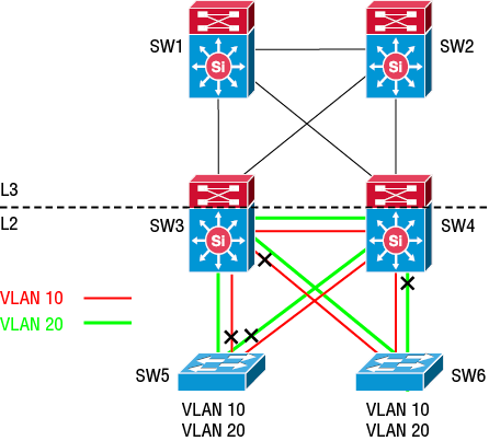
Looped and loop-free topologies differ from each other in terms of resiliency. In the looped topology, you deliberately configure physical loops, and Spanning Tree prevents bridging loops from occurring by blocking some of those redundant logical connections. The looped triangle, shown in Figure 3.6, is the most common example of a looped topology.
Notice that in the looped triangle, each access switch is connected to both distribution switches. If you were to add another access switch, it would consume at least two additional ports on the distribution switches. When a logical link failure occurs, Spanning Tree reconverges, unblocking those previously blocked links to allow traffic to flow freely. To put it simply, you're relying on Spanning Tree to provide resiliency. Again, this is convenient, but the price you pay is that reconvergence in the face of a logical link failure can take several seconds. Another downside is that you waste some port space due to blocking. However, if you have multiple VLANs, you can overcome this somewhat by load-balancing VLANs across different links.
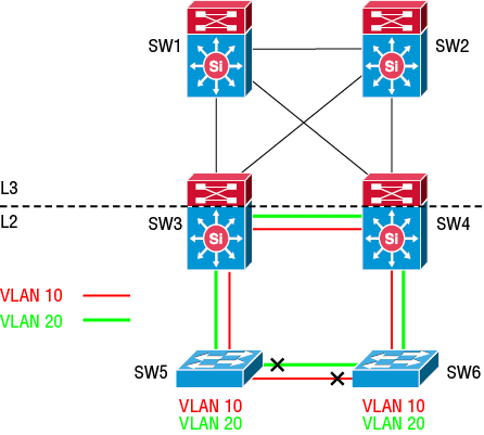
The looped square, shown in Figure 3.7, consumes fewer switchports on the distribution switches. In this case, each access switch connects to only one distribution switch and one access switch. Adding another access switch would thus consume at least one additional port on just one distribution switch. Hence, if you need a VLAN to span multiple access switches but your distribution switch port space is at a premium, you may want to consider this setup. But keep in mind that the looped square carries with it the additional disadvantage that a logical link failure or misconfiguration could cause traffic to start flowing horizontally through an access switch, leading to an inefficient use of bandwidth.
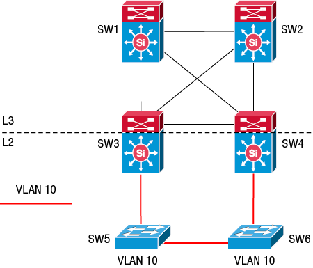
In the loop-free topologies, you avoid configuring physical loops in the access and distribution layers so that bridging loops aren't possible. You'll still run Spanning Tree just in case, but you won't depend on it. One aspect of the loop-free topologies is that they don't consume much port space on the distribution switches. There are a few ways to configure a loop-free topology, but the one shown in Figure 3.8 stands out above the rest and is the one Cisco recommends.
This particular topology allows simultaneous use of all links and provides some resiliency in case of a distribution switch failure. The only consideration is that no VLAN can span more than two access switches, but as you already know, limiting the size of a broadcast domain isn't a bad thing. Note that the connections in the core layer are looped, which isn't a problem because those connections are all routed.
Loop-Free U-Topologies
If you think you'll ever need to extend a VLAN to more than one access switch, consider one of the loop-free U-topologies, named for the distinctive U shape of the layer 2 domain. The loop-free U-topology, as shown in Figure 3.9, lets you span a VLAN between two access switches. The failure of a distribution switch will send all traffic through another access switch, but you won't lose connectivity. Notice that the connections between the distribution switches are layer 3.
If you want to extend a VLAN to more than two switches, the loop-free inverted-U topology in Figure 3.10 lets you do so at the cost of sacrificing resiliency. If a distribution switch fails, its connected access switches will lose all upstream connectivity. To achieve the upside-down U shape, the connections between the distribution switches are layer 2, whereas connections between access switches are absent.
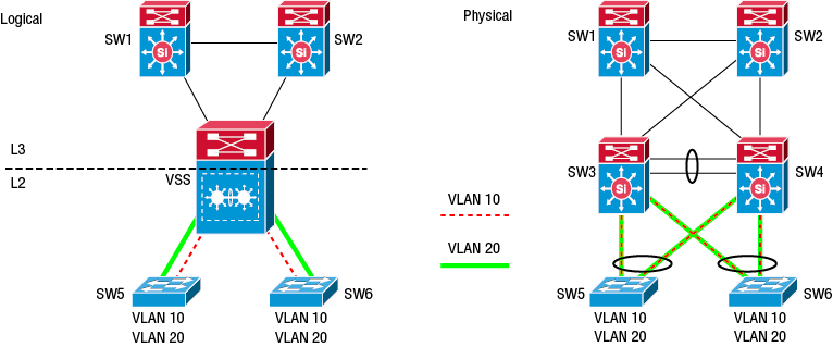
The virtual switching system (VSS) allows two switches to operate as a single logical switch. By implementing VSS and EtherChannels in a virtual switched topology, you can remove layer 2 loops while still using all available links. (EtherChannels let you combine physical interfaces into a single logical interface. We'll cover EtherChannels in a moment). This essentially gives you the advantages of a loop-free topology while making efficient use of bandwidth. The only disadvantage is that it requires switches that support the VSS. Figure 3.11 illustrates the logical and physical layout of a virtual switch topology.
You'll notice that the physical topology looks just like the looped triangle from Figure 3.6. Although the underlying physical topologies are the same, the VSS topology is logically quite different in that it's loop-free and doesn't have any blocked links.
In the VSS topology, both distribution switches are physically connected together using a set of links bundled into a single logical EtherChannel. This logical connection is called the virtual switch link (VSL). When you configure VSS, one switch becomes the active switch and the other is the standby. The active switch handles all configured layer 2 and layer 3 protocols, such as Spanning Tree and dynamic routing protocols. The active switch replicates configuration information to the standby so that it's ready to take over control in the event the active switch fails.
Notice that each access switch is physically connected to both the active and standby switches. Each pair of ports is configured as an EtherChannel, allowing the access switch to utilize both physical connections, treating them as a single logical port. On the VSS side, these connections are configured as multichassis EtherChannels (MECs). This allows all links to be forwarding and precludes the need for Spanning Tree to block any links. Also, in the event of a switch failover, this configuration will allow traffic to keep flowing with minimal interruption.
Keep in mind that VSS doesn't require you to connect access switches to the distribution switches using EtherChannels. You can still implement a looped topology between the access and distribution switches and depend on Spanning Tree to block one of the redundant links. But during a switch failover, you'll be waiting on Spanning Tree to reconverge, which can take much longer.
Stateful switchover is a feature that synchronizes state information such as the FIB and CEF adjacencies between the active and standby switches. Virtual switching thus eliminates the need to run a first-hop redundancy protocol, since both switches function as a single switch. You configure endpoints with the virtual switch's IP as the default gateway. In the event one switch fails, stateful switchover occurs seamlessly, allowing IP forwarding to continue without interruption in a process called non-stop forwarding (NSF). The switchover typically takes anywhere from less than one second to three seconds.
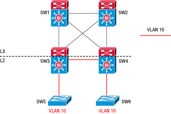
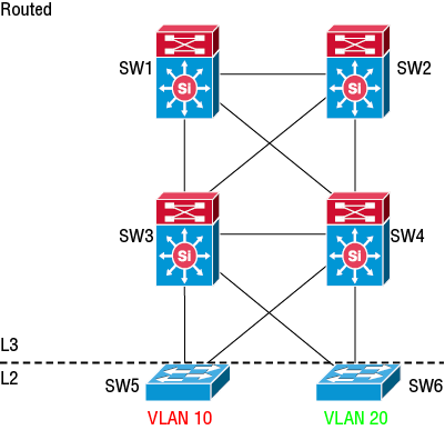
Routed Access Topology
The routed access topology, shown in Figure 3.12, is the best choice all-around. You get rapid convergence times, load balancing, efficient use of all links, stability, and scalability. In a routed topology, a VLAN can't span more than a single access switch, thus each access switch must serve as the default gateway for its respective VLAN. This means there's no need for a first-hop redundancy protocol (FHRP) and no risky bridging loops. Unlike a switched topology, the routed access topology is not very susceptible to a catastrophic meltdown. The only downside is that it's a bit more complex to configure up front, considering you have to allocate two private IP addresses for each point-to-point routed link. Additionally, you'll need to configure a dynamic routing protocol, such as OSPF or EIGRP. We'll cover those in Chapter 5, “Open Shortest Path First (OSPF),” and Chapter 6, “Enhanced Interior Gateway Routing Protocol (EIGRP).”
EtherChannels provide redundancy and increased bandwidth by letting you combine up to eight physical interfaces into a single logical interface called a port channel. You can also have eight backup links that can take over if one of the active links fails. This means that, for example, with four 1 Gbps interfaces, you can push up to 4 Gbps through a single port channel. It also lets you hide the physical ports from Spanning Tree and instead present a single logical interface, avoiding the nasty problem of blocking and slow reconvergence times.
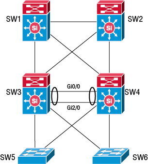
Consider the physical topology in Figure 3.13. There are two links between the distribution switches, SW3 and SW4. Without EtherChannel configured, Spanning Tree will block one of these ports. However, by configuring EtherChannel, each switch and any protocols running on it—including Spanning Tree—will view the port pair as a single logical interface.
Rather than splitting up an Ethernet frame, sending pieces across all four links, and having the opposite end reassemble them, EtherChannel takes a much simpler approach. It uses a hash algorithm—the load-balancing method—to determine which frames to forward over a particular link. The load-balancing method can create a hash based on the source MAC, source IP, destination MAC, or destination IP in a frame. There are six load-balancing methods that you can configure on a per-switch basis, as follows:
SW3(config)#port-channel load-balance ?
  dst-ip       Dst IP Addr
  dst-mac      Dst Mac Addr
  src-dst-ip   Src XOR Dst IP Addr
  src-dst-mac  Src XOR Dst Mac Addr
  src-ip       Src IP Addr
  src-mac      Src Mac Addr
By default, the switch determines which link to use based only on the source MAC. This is called the source MAC load-balancing mode. To understand how it works, suppose that SW3 receives a frame with the source MAC address 0123.4567.0002, and the frame is addressed to a device that's reachable via SW4, which is on the other end of a port channel. SW3 will hash the source MAC address, and based on the output, will send the frame out of either Gi0/0 or Gi2/0.
In addition to source MAC, there are five other load-balancing methods you can choose from: destination MAC, source IP, destination IP, source IP XOR with the destination IP, and source MAC XOR with the destination MAC. The XOR, or eXclusive OR, methods hash the source and destination addresses together. To understand how to decide which one to choose, consider the port channel between SW4 and SW5. Suppose you have a workstation connected to SW4 and two servers connected to SW5. All are in the same VLAN. The workstation needs to download data from both servers. Because the workstation will be sending frames addressed to different servers, the best load-balancing methods for SW4 would be destination MAC or destination IP. The best load-balancing method for SW5, on the other hand, would be source MAC or source IP, since traffic from the servers is coming from two different MAC and IP addresses.
Configuring a working EtherChannel is not a one-sided operation. You have to perform the appropriate configuration on both ends of the link. To configure an EtherChannel, you select a group of ports you want to combine into a single port channel interface. This group of ports is called the port channel group, and each individual port within the group is a member port. After you decide the ports you want to join together in an EtherChannel, you must configure the EtherChannel mode. There are three different modes:
Static (on)
Port Aggregation Protocol (PAgP)
Link Aggregation Control Protocol (LACP)
Static EtherChannels
Static, or “on,” mode unconditionally places the selected ports into a port channel group, no questions asked. As long as you configure both sides with the same parameters, everything should work fine.
Whenever you are configuring a port channel, it's crucial that all member ports be configured with the same parameters, such as trunk status, trunk encapsulation, speed, and duplex. The port channel will inherit its configuration from the physical interfaces. It's easy to inadvertently create bridging loops by configuring a port channel on one side but not on the other. In that case, Spanning Tree will block one of the links. Thus, it's also a good idea to shut down the ports before creating a port channel to avoid bridging loops.
Each port channel group is identified by a channel group number. Channel group numbers are locally significant and must be unique per switch, but they don't have to match on both ends. However, to avoid confusion, it's a good idea to use the same number on both ends for identification. Let's start by configuring SW3. First, we'll set Gi0/0 and Gi2/0 to their defaults.
SW3(config)#default interface range gigabitEthernet 0/0, gigabitEthernet 2/0SW3(config)#int range gigabitEthernet 0/0, gigabitEthernet 2/0! Shutdown the portsSW3(config-if-range)#shutdown
SW3(config-if-range)#channel-group 1 mode on! Verify the configurationSW3(config-if-range)#do show etherchannel 1 summaryFlags: D - down P - bundled in port-channel I - stand-alone s - suspended H - Hot-standby (LACP only) R - Layer3 S - Layer2 U - in use N - not in use, no aggregation f - failed to allocate aggregator M - not in use, minimum links not met m - not in use, port not aggregated due to minimum links not met u - unsuitable for bundling w - waiting to be aggregated d - default port A - formed by Auto LAGNumber of channel-groups in use: 1Number of aggregators: 1Group Port-channel Protocol Ports------+-------------+-----------+-----------------------------------------------1 Po1(SD) - Gi0/0(D) Gi2/0(D)
The “D” in parentheses means “down” because the ports are shut down. Hence, the port-channel interface is down also. Now let's perform the same configuration on SW4:
SW4(config)#default interface range gigabitEthernet 0/0, gigabitEthernet 2/0SW4(config)#int range gi0/0, gi2/0SW4(config-if-range)#shutdownSW4(config-if-range)#switchport trunk encapsulation dot1qSW4(config-if-range)#switchport mode trunkSW4(config-if-range)#channel-group 1 mode onCreating a port-channel interface Port-channel 1
Now, we'll bring the interfaces back up.
SW4(config-if-range)#no shutdownSW4(config-if-range)#%LINK-3-UPDOWN: Interface GigabitEthernet0/0, changed state to up%LINK-3-UPDOWN: Interface GigabitEthernet2/0, changed state to up%LINEPROTO-5-UPDOWN: Line protocol on Interface GigabitEthernet2/0, changed state to up%LINEPROTO-5-UPDOWN: Line protocol on Interface GigabitEthernet0/0, changed state to up%LINK-3-UPDOWN: Interface Port-channel1, changed state to up%LINEPROTO-5-UPDOWN: Line protocol on Interface Port-channel1, changed state to up
Notice that after bringing the member interfaces back up, the port channel interface Port-channel1 comes up as well. The interfaces on the opposite end at SW3 are shut down, but because we've configured a static EtherChannel, SW4 doesn't do any checking to determine whether SW3's port channel is active. Let's jump back to SW3 and reenable the ports there:
SW3(config-if-range)#no shutSW3(config-if-range)#%LINK-3-UPDOWN: Interface GigabitEthernet0/0, changed state to up%LINK-3-UPDOWN: Interface GigabitEthernet2/0, changed state to up%LINEPROTO-5-UPDOWN: Line protocol on Interface GigabitEthernet0/0, changed state to up%LINEPROTO-5-UPDOWN: Line protocol on Interface GigabitEthernet2/0, changed state to up%LINK-3-UPDOWN: Interface Port-channel1, changed state to up%LINEPROTO-5-UPDOWN: Line protocol on Interface Port-channel1, changed state to up! Verify the configurationSW3(config-if-range)#do show etherchannel 1 summaryFlags: D - down P - bundled in port-channel I - stand-alone s - suspended H - Hot-standby (LACP only) R - Layer3 S - Layer2 U - in use N - not in use, no aggregation f - failed to allocate aggregator M - not in use, minimum links not met m - not in use, port not aggregated due to minimum links not met u - unsuitable for bundling w - waiting to be aggregated d - default port A - formed by Auto LAGNumber of channel-groups in use: 1Number of aggregators: 1Group Port-channel Protocol Ports------+-------------+-----------+-----------------------------------------------1 Po1(SU) - Gi0/0(P) Gi2/0(P)
The “SU” in parentheses next to Po1 indicates that this is a layer 2 (switched) interface rather than a layer 3 (routed) interface. The port channel will inherit the characteristics of the parent interfaces. For example, if Gi0/0 and Gi2/0 were routed interfaces, Po1 would be a routed (layer 3) interface as well.
SW3(config-if-range)#do show interfaces port-channel1 trunkPort Mode Encapsulation Status Native vlanPo1 on 802.1q trunking 1Port Vlans allowed on trunkPo1 1-4094Port Vlans allowed and active in management domainPo1 1,10,20Port Vlans in spanning tree forwarding state and not prunedPo1 1,10,20
To remove a static port channel configuration, just delete the interface as follows:
SW3(config)#no interface po1SW3(config)#! To avoid creating bridging loops, IOS will shut down the member interfaces.%LINK-5-CHANGED: Interface GigabitEthernet0/0, changed state to administratively down%LINK-5-CHANGED: Interface GigabitEthernet2/0, changed state to administratively down%LINEPROTO-5-UPDOWN: Line protocol on Interface GigabitEthernet0/0, changed state to down%LINEPROTO-5-UPDOWN: Line protocol on Interface GigabitEthernet2/0, changed state to down
Port Aggregation Control Protocol
PAgP is a Cisco-proprietary protocol that attempts to negotiate a port channel with a connected switch. PAgP first performs some sanity checks to make sure both ends are compatible before creating the EtherChannel. If any pair of ports aren't compatible due to a mismatched speed, duplex, native VLAN, or trunk encapsulation, PAgP will still attempt to form an EtherChannel with the remaining ports that are compatible.
PAgP has two modes: Auto and Desirable. In Desirable mode, the switch will actively attempt to form an EtherChannel. In Auto mode, it will not actively try to negotiate a port channel. However, if the other side is set to Desirable mode, then the switch set to Auto will negotiate the port channel. Table 3.3 lists how the combination of configuration modes determines whether a port channel will form.
You may find it helpful to remember the Auto and Desirable modes by remembering that Ag (as in PAgP) is the chemical symbol for silver, and silver is automatically desirable. It's cheesy, but it works for me! The configuration commands for PAgP are similar to those of a static EtherChannel, as follows:
! SW4 has already been configured in Desirable mode. Now we'll configure SW3 to use! Desirable mode.SW3(config)#int range gi0/0,gi2/0SW3(config-if-range)#channel-group 1 mode ? active Enable LACP unconditionally auto Enable PAgP only if a PAgP device is detected desirable Enable PAgP unconditionally on Enable Etherchannel only passive Enable LACP only if a LACP device is detected
We'll choose Desirable mode. We could also choose Auto mode and it would establish a port channel since the other side is set to Desirable.
SW3(config-if-range)#channel-group 1 mode desirableCreating a port-channel interface Port-channel 1
The member interfaces are shut down, so we'll bring them up.
SW3(config-if-range)#no shut%LINK-3-UPDOWN: Interface GigabitEthernet0/0, changed state to up%LINK-3-UPDOWN: Interface GigabitEthernet2/0, changed state to up%LINEPROTO-5-UPDOWN: Line protocol on Interface GigabitEthernet0/0, changed state to up%LINEPROTO-5-UPDOWN: Line protocol on Interface GigabitEthernet2/0, changed state to up%LINEPROTO-5-UPDOWN: Line protocol on Interface Port-channel1, changed state to up! Verify the configurationSW3(config-if-range)#do show etherchannel 1 summaryFlags: D - down P - bundled in port-channel I - stand-alone s - suspended H - Hot-standby (LACP only) R - Layer3 S - Layer2 U - in use N - not in use, no aggregation f - failed to allocate aggregator M - not in use, minimum links not met m - not in use, port not aggregated due to minimum links not met u - unsuitable for bundling w - waiting to be aggregated d - default port A - formed by Auto LAGNumber of channel-groups in use: 1Number of aggregators: 1Group Port-channel Protocol Ports------+-------------+-----------+-----------------------------------------------1 Po1(SU) PAgP Gi0/0(P) Gi2/0(P)
Link Aggregation Control Protocol
LACP is an open standard protocol that performs essentially the same function as PAgP. Note that LACP and PAgP are not compatible with each other, so you must use the same protocol on both ends.
You can configure LACP to operate in two modes: Active or Passive. In Active mode, the switch will actively try to negotiate a port channel. In Passive mode, it won't actively try to negotiate a port channel, but if the other end is set to Active, then both switches will form a port channel. Table 3.4 lists the outcomes of the different mode combinations.
Configuring LACP is almost identical to configuring PAgP. In the following example, we configure SW4 to use LACP in Active mode:
! SW3 is already configured for LACP Active mode.SW4(config)#int range gi0/0,gi2/0SW4(config-if-range)#channel-group 1 mode activeCreating a port-channel interface Port-channel 1%LINEPROTO-5-UPDOWN: Line protocol on Interface Port-channel1, changed state to upSW4(config-if-range)#do show etherchannel 1 summaryFlags: D - down P - bundled in port-channel I - stand-alone s - suspended H - Hot-standby (LACP only) R - Layer3 S - Layer2 U - in use N - not in use, no aggregation f - failed to allocate aggregator M - not in use, minimum links not met m - not in use, port not aggregated due to minimum links not met u - unsuitable for bundling w - waiting to be aggregated d - default port A - formed by Auto LAGNumber of channel-groups in use: 1Number of aggregators: 1Group Port-channel Protocol Ports------+-------------+-----------+-----------------------------------------------1 Po1(SU) LACP Gi0/0(P) Gi2/0(P)
First-Hop Redundancy Protocols
Recall that in a switched topology, the default gateway for a VLAN typically will run on one of the two distribution switches. But ideally, you'd run a FHRP so that either one can serve as the default gateway. That way, if one switch fails, the other can take over without requiring any reconfiguration, and hosts can still reach their configured default gateway. FHRPs include
Hot Standby Router Protocol (HSRP)
Virtual Router Redundancy Protocol (VRRP)
Gateway Load Balancing Protocol (GLBP)
When a host needs to reach a different IP subnet, it has to traverse a gateway or router. In most cases a host will have only one default gateway IP configured. Suppose the default gateway for a server is 1.1.1.1. If that server needs to send an IP packet to 2.2.2.2, it takes the IP packet, encapsulates it inside an Ethernet frame, and then addresses the frame to the default gateway's MAC address. If the default gateway goes down, the server won't be able to reach any other subnets.
This is where FHRPs come in. When you use VRRP, HSRP, or GLBP, you can have multiple gateways that share a single virtual IP address that you configure on hosts as the default gateway. If one of the gateways goes down, one of the others will take over, allowing hosts to continue to communicate outside the subnet.
In a switched topology, you configure IP routing protocols and FHRPs on layer 3 switches. But you can configure them on routers, too.
Hot Standby Router Protocol
HSRP is a Cisco-proprietary protocol that currently comes in two versions: version 1 and version 2. Version 1, described in RFC 2281 (www.ietf.org/rfc/rfc2281), is the default. The biggest practical difference between the two versions is that only version 2 supports IPv6. From a configuration and operation perspective, however, they're pretty much the same. If you consider using version 2, keep in mind that the versions aren't cross-compatible.
Here's how it works. Suppose that SW3 and SW4 both have SVIs in VLAN 30. SW3 is 3.3.3.3/24, and SW4 is 3.3.3.4/24. To configure HSRP to provide a highly available default gateway for the 3.3.3.0/24 subnet, you'd configure both SVIs to be part of the same HSRP group. You identify the HSRP group by a number between 0 and 255. When you configure an HSRP group, you must specify a virtual IP address, which is the IP that hosts in the subnet will use for their default gateway. The virtual IP resolves to a virtual MAC address in the format 0000.0c07.acxx, xx being the group number in hexadecimal. For example, if you use group number 3, the last part of the MAC address is ac03. HSRP peers communicate with one another using the “all routers” multicast address 224.0.0.2.
HSRP uses an active-passive configuration. The active router listens on the virtual IP address, and the other router is the standby. With HSRP, the router with the highest priority will become active. If the priorities of all routers in the group are equal, then the router with the highest IP will be the active router. All other routers in the group are standby.
In the following example, we'll configure SW3 and SW4 with SVIs for the 3.0.0.0/24 subnet in VLAN 30 and place them both in HSRP group 3. The virtual IP address will be 3.3.3.254, which is what hosts should use as their default gateway. We'll then configure the priority on SW3 to be higher, so it becomes the active router. Lastly, we'll configure MD5 authentication. Let's begin on SW3.
! Configure the SVISW3(config)#int vlan 30SW3(config-if)#ip address 3.3.3.3 255.255.255.0
We'll create HSRP group 3 with the virtual IP address 3.3.3.254.
SW3(config-if)#standby 3 ip 3.3.3.254
Let's set the priority to the highest possible value to ensure SW3 is the active router.
SW3(config-if)#standby 3 priority 255
Next, let's configure MD5 authentication.
SW3(config-if)#standby 3 authentication md5 key-string 1337$ecr37! Verify the configurationSW3(config-if)#do show standbyVlan30 - Group 3 State is Active Virtual IP address is 3.3.3.254 Active virtual MAC address is 0000.0c07.ac03 (MAC In Use) Local virtual MAC address is 0000.0c07.ac03 (v1 default) Hello time 3 sec, hold time 10 sec Next hello sent in 2.304 secs Authentication MD5, key-string Preemption disabled Active router is local Standby router is unknown Priority 255 (configured 255) Group name is "hsrp-Vl30-3" (default)
Now let's create the corresponding configuration on SW4:
SW4(config)#int vlan 30SW4(config-if)#ip address 3.3.3.4 255.255.255.0SW4(config-if)#standby 3 ip 3.3.3.254SW4(config-if)#standby 3 authentication md5 key-string 1337$ecr37SW4(config-if)#do show standbyVlan30 - Group 3 State is Standby Virtual IP address is 3.3.3.254 Active virtual MAC address is 0000.0c07.ac03 (MAC Not In Use) Local virtual MAC address is 0000.0c07.ac03 (v1 default) Hello time 3 sec, hold time 10 sec Next hello sent in 0.272 secs Authentication MD5, key-string Preemption disabled Active router is 3.3.3.3, priority 255 (expires in 8.752 sec) Standby router is local Priority 100 (default 100) Group name is "hsrp-Vl30-3" (default)
A quick and dirty way to verify the configuration is working is to ping the virtual IP address from anywhere other than the active router.
SW4(config-if)#do ping 3.3.3.254Type escape sequence to abort.Sending 5, 100-byte ICMP Echos to 3.3.3.254, timeout is 2 seconds:.!!!!Success rate is 80 percent (4/5), round-trip min/avg/max = 4/9/17 ms
Virtual Router Redundancy Protocol
The VRRP, defined in RFC 3768 (https://tools.ietf.org/html/rfc3768) is an open-standard FHRP that operates much the same as HSRP. Also like it, VRRP uses a group number, a virtual IP address, and a virtual MAC address. But in this case, the MAC address is 0000.5e00.01xx, with xx being the group number in hexadecimal. VRRP routers communicate with one another using the reserved multicast address 224.0.0.18.
In VRRP, the master router listens on the virtual IP address and virtual MAC address. The other routers are called the backups. One significant difference between VRRP and HSRP is that with VRRP the virtual IP address can be the same as one of the interface IPs. This makes it easier to implement VRRP in an existing topology without having to modify the hosts’ currently configured default gateway. For example, if hosts are using the default gateway 192.168.7.1, you can continue to use that IP without readdressing any interfaces. The following example shows how this is done on SW3:
SW3(config)#int vlan 30SW3(config-if)#ip address 3.3.3.3 255.255.255.0SW3(config-if)#vrrp 30 ip 3.3.3.3SW3(config-if)#%VRRP-6-STATECHANGE: Vl30 Grp 30 state Init -> Master%VRRP-6-STATECHANGE: Vl30 Grp 30 state Init -> MasterSW3(config-if)#do show vrrpVlan30 - Group 30 State is Master Virtual IP address is 3.3.3.3 Virtual MAC address is 0000.5e00.011e Advertisement interval is 1.000 sec Preemption enabled Priority is 255 Master Router is 3.3.3.3 (local), priority is 255 Master Advertisement interval is 1.000 sec Master Down interval is 3.003 sec
SW3 is the master. Notice that the priority is set to 255. As with HSRP, in VRRP, the router with the highest priority wins. Note that in this case, SW3's SVI address is the same as the virtual IP address. This means SW3 is the address owner. In this situation, SW3 sets its own priority to 255, the highest possible value, thus ensuring that it's the master as long as the interface is up. Now let's configure SW4:
SW4(config)#int vlan 30SW4(config-if)#ip address 3.3.3.4 255.255.255.0SW4(config-if)#vrrp 30 ip 3.3.3.3SW4(config-if)#%VRRP-6-STATECHANGE: Vl30 Grp 30 state Init -> Backup%VRRP-6-STATECHANGE: Vl30 Grp 30 state Init -> BackupSW4(config-if)#do show vrrpVlan30 - Group 30 State is Backup Virtual IP address is 3.3.3.3 Virtual MAC address is 0000.5e00.011e Advertisement interval is 1.000 sec Preemption enabled Priority is 100 Master Router is 3.3.3.3, priority is 255 Master Advertisement interval is 1.000 sec Master Down interval is 3.609 sec (expires in 2.730 sec)
SW4 is the backup. Because SW4 isn't the IP address owner, it assumes the default priority of 100.
Gateway Load-Balancing Protocol
GLBP is another Cisco-proprietary protocol that provides first-hop redundancy by load-balancing traffic across multiple gateways. You may want to use GLBP if you have a lot of traffic and want to spread the load among multiple smaller routers. Just place them together in a GLBP group and they can function as a single virtual router. Routers in a GLBP group use the multicast address 224.0.0.102.
Just as with HSRP and VRRP, a GLBP group has a virtual IP address that hosts use as their configured default gateway. In a GLBP group, one router serves as the active virtual gateway (AVG), whereas all routers in the group function as the active virtual forwarder (AVF), or just forwarder for short. Every router in the group listens on a virtual MAC address in the format 0007.B400.xxyy, where xx is the group number and yy is the forwarder number. You can have up to four virtual MAC addresses in a group. If there are more than four routers in a GLBP group, the additional routers will function as secondary AVFs, ready to take over in case a primary AVF fails.
The AVG listens for ARP requests for the virtual IP address. Here's where the load balancing part comes in and how GLBP differs from HSRP and VRRP. Instead of responding to the ARP request with a single virtual MAC address that all routers share, the AVG responds with the virtual MAC address of one of the forwarders in the group. Using the default round-robin load-balancing method, each time the AVG receives an ARP request for the virtual IP address, it replies with a different virtual MAC address. The actual router a host uses as its default gateway can change based on the MAC address that it receives in the ARP reply from the AVG.
To understand this better, consider a simple example. Suppose you configure a GLBP group on two switches, Switch A and Switch B, configured in that order. Both switches are in GLBP group 5 and have a virtual IP address of 192.168.5.254.
Switch A's virtual MAC address would be 0007.B400.0501, indicating a group number of 5 and a forwarder number of 1.
Switch B's virtual MAC address would be 0007.B400.0502, indicating group 5 and forwarder 2.
Both routers are AVFs. But which one is the AVG? The AVG is elected based on the highest priority, the default priority being 100. Valid priorities range from 1 to 255. If the priorities of all routers are tied, then the one with the highest IP address wins. In the preceding example, Switch A would be the AVG since it was configured first. Since Switch A is the AVG, it will listen for ARP requests for the virtual IP address 192.168.5.254. It will respond with one of the virtual MAC addresses of an AVF, 0007.B400.0501 or 0007.B400.0502.
By default, once a router becomes the AVG, it will remain the AVG as long as it's up. Even if you later configure another router with a higher priority, the first configured router will remain the AVG. You can overcome this behavior by enabling preemption. With preemption enabled, the router with the highest priority will always take over as the AVG.
There are three load-balancing methods you can configure with GLBP:
Round-robin—The AVG will cycle through the group, replying with the virtual MAC address of each AVF in order. This is the default method.
Weighted—You configure a weight (1–254) on each AVF, indicating the ratio of traffic you want each gateway to handle. For example, if you want Switch A to handle 80 percent of the traffic and Switch B to handle 20 percent, you'd configure Switch A with a weight of 80 and Switch B with a weight of 20.
Host-dependent—Each host MAC address is mapped to a specific AVF so that the host will always use that AVF as its default gateway.
If you don't want to use the default round-robin method, you should configure the load-balancing method on any switch that might become the AVG. Not surprisingly, the commands to configure GLBP mirror those of VRRP and HSLP. The following example shows how to configure GLBP group 3 with a virtual IP address of 3.3.3.254. We'll give SW4 a weighting of 80 and enable preemption so it's always the AVG:
SW4(config)#int gi0/0! Configure GLBP group 3 with the virtual IP address 3.3.3.254.SW4(config-if)#glbp 3 ip 3.3.3.254! Set the priority to 255 so that SW4 is always the AVGSW4(config-if)#glbp 3 priority 255! Set the load-balancing method to weightedSW4(config-if)#glbp load-balancing weighted! Set the weight to 80SW4(config-if)#glbp 3 weighting 80! Enable preemption so SW4 is always the AVGSW4(config-if)#glbp 3 preempt
We'll then configure SW3 and give it a weighting of 20:
SW3(config)#int gi0/0SW3(config-if)#glbp 3 ip 3.3.3.254SW3(config-if)#glbp load-balancing weighted! Set the weight to 20SW3(config-if)#glbp 3 weighting 20
Summary
The physical network layout determines what path traffic can take, so it's tempting to assume that creating a full mesh of connections between switches would be the perfect framework for maximizing bandwidth and resiliency. But this approach leaves out an important consideration: scalability. A network is by definition a distributed system, and its whole purpose is to move data between applications, wherever they may happen to live. As a rule, the number of applications and hence the number of devices will inevitably grow. Therefore, scalability is the most important consideration when it comes to designing your physical network. That's why a modular approach using a three-tier architecture is always going to be your best bet. However, in a smaller network that's not expected to grow much, a two-tier collapsed core is a good lower-cost alternative.
Regardless of the physical topology, the layer 2 topology you choose will make all the difference when it comes to actual traffic patterns. As with the physical topology, you're concerned with performance, reliability, and scalability. And you can certainly achieve all three. But because the layer 2 topology is just determined by device configuration, you also need to consider configuration complexity.
Switched topologies that make heavy use of transparent bridging are naturally easier to manage. But with the exception of the virtual switch topology, all switched topologies make inefficient use of bandwidth. They also carry the potential for asymmetric routing, which can result in suboptimal use of bandwidth and can make troubleshooting issues a bit more complicated. Switched topologies are divided into three classes: looped, loop-free, and virtual switching. Looped topologies let you extend a VLAN to a practically unlimited number of switches while still maintaining some resiliency. They also waste bandwidth thanks to Spanning Tree blocking redundant links, and they consume more ports on your distribution switches. Loop-free topologies make use of all available links but are less resilient.
Routed and VSS topologies are comparable in that they give you maximum bandwidth, resiliency, and scalability. The big difference between the two is that in a routed topology, a VLAN can exist on only one access switch. This actually makes the routed topology more stable and easier to troubleshoot.
EtherChannels provide a silver lining for switched topologies in particular, allowing you to use redundant physical links without worrying about Spanning Tree blocking them. It's important to note that using EtherChannels in a looped topology will still result in some links being blocked. But EtherChannels aren't good only for switched topologies. You can also use EtherChannels in a routed topology by placing routed interfaces into a port channel group.
If you go with a switched topology other than VSS, the FHRPs VRRP, HSRP, and GLBP are a necessary hack to ensure that your hosts can maintain reachability to other subnets if one of your distribution switches fails. This isn't an issue in a VSS topology because both distribution switches function as a single logical switch, so the failure of one switch is essentially transparent to the hosts. In a similar vein, a routed topology doesn't need an FHRP because the dynamic routing protocols running on the switches will detect and route around link failures.
Exam Essentials
Know the functions of the layers in the two-tier and three-tier architectures. The three-tier architecture consists of a core layer, distribution/aggregation layer, and access layer. The two-tier architecture collapses the core and distribution layer into a single layer called a collapsed core.
Know the difference between switched (layer 2) and routed (layer 3) interfaces. A switched interface is a VLAN access or trunk port and can't have an IP address assigned. A routed interface has no VLAN and can have an IP address assigned to it.
Understand the common layer 2 topologies. Switched topologies include looped, loop-free, and VSS. The routed topology eliminates spanned VLANs and instead places each interswitch link into a separate broadcast domain.
Be able to configure layer 2 and layer 3 EtherChannels. An EtherChannel can consist of 1–8 active links. You can create a static port channel or let LACP or PAgP negotiate one for you. The difference between a layer 2 and a layer 3 EtherChannel is determined by whether the member interfaces are switched or routed.
Be able to configure the first-hop redundancy protocols. The configuration semantics of VRRP, HSRP, and GLBP are strikingly similar, often differing by only one word. I suggest mastering VRRP first. You'll then be able to transfer much of that knowledge to HSRP and GLBP.
Review Questions
You can find the answers in the appendix.
Which of the following best describes traffic between a database server and a web server?
North-South
East-West
Client-server
Intra-VLAN
Which of the following best describes traffic between an IP phone and a DNS server?
North-South
East-West
Point-to-point
Inter-VLAN
Which of the following is the most scalable physical architecture for North-South traffic patterns?
Leaf-and-spine architecture
Two-tier collapsed core
Three-tier
Routed
Which of the following layers should always be routed?
Access
Aggregation
Distribution
Core
Which of the following should be in the same distribution block? (Choose two.)
Web application load balancer
An IP phone
A web server
An Internet router
Which of the following is true regarding a routed interface on a switch?
It must be assigned an IP address.
It consumes one VLAN.
It can be configured as a trunk port.
It can be assigned two IP addresses.
Which of the following layer 2 topologies let you span a VLAN across more than two switches? (Choose two.)
Looped
Loop-free U
Loop-free inverted-U
Routed
Which of the following is true of using a VSS topology?
You should disable Spanning Tree when using VSS.
There's no need to run a FHRP.
Access switches must connect to the virtual switch using multichassis EtherChannels.
The active and standby both perform IP routing to avoid asymmetric routing.
Given two distribution switches and one VLAN that spans four access switches, which layer 2 topology will consume the fewest number of ports on the distribution switches?
Looped triangle
Looped square
Routed
Loop-free U
What are two differences between the VSS topology and the looped triangle? (Choose two.)
The looped triangle can't use EtherChannels.
The looped triangle has blocked links.
The VSS requires access switches to be directly connected to one another.
The VSS has no links blocking.
On Switch A, you issue the channel-group 7 mode on command on a range of interfaces. Which command, if configured on the facing switch's links, will result in a working EtherChannel?
channel-group 7 mode active
channel-group 1 mode on
channel-group 7 mode desirable
port-group 7 mode on
You've configured a pair of links to use LACP Active mode. Configuring which of the following configuration commands on the facing switch will form an EtherChannel?
channel-group 2 mode passive
channel-group 3 mode on
channel-group 4 mode auto
channel-group 3 mode desirable
Up to how many active ports can you have in an EtherChannel?
1
4
8
16
How many backup ports can you have in an EtherChannel?
1
4
8
16
Which of the following modes is PAgP compatible with?
On
Active
Passive
Auto
Which of the following can result in a VRRP router having a priority of 255?
Preemption is enabled.
The default priority is 255.
It's the first router configured in the group.
The router is the group's IP address owner.
What is the default priority for HSRP?
0
100
254
255
Which protocol uses the multicast address 224.0.0.2?
HSRP
VRRP
GLBP
LACP
What's the virtual MAC address format for VRRP?
0000.5e00.01xx, with xx being the group number in hexadecimal
0000.5e00.01xx, with xx being the group number in decimal
0007.B400.01xx, with xx being the group number in hexadecimal
0007.0c07.acxx, with xx being the forwarder number in hexadecimal
Which of the following is true of GLBP? (Choose two.)
There can be multiple active AVGs at a time.
An AVG can be an AVF.
There can be multiple active AVFs at a time.
You configure the load-balancing method on each AVF.
Which of the following modes is LACP compatible with? (Choose two.)

 Ultimately, the performance and flexibility of any network hinges on the physical topology—that is, the physical connectivity between devices. After that, every subsequent decision is a logical configuration decision that depends in some way on the physical topology. In other words, the physical topology determines the path traffic can take, but the logical layer 2 topology determines what path the traffic will take. In this chapter, we'll look at how different layer 2 designs influence traffic patterns, which in turn influence bandwidth and reliability. We'll then turn to EtherChannels, which can help you make efficient use of your physical links as well as make your network resilient to link failures. Finally, we'll cover three first-hop redundancy protocols that let you create a highly available default gateway for hosts in a subnet.