THE CCNP ENCOR EXAM OBJECTIVES COVERED IN THIS CHAPTER INCLUDE THE FOLLOWING:
Domain 1: Architecture
✓ 1.2 Analyze design principles of a WLAN deployment
Domain 3: Infrastructure
✓ 3.3 Wireless
Domain 5: Security
✓ 5.4 Configure and verify wireless security features
✓ 5.5 Describe the components of network security design
There was a time when being a network engineer meant having to understand how data is converted into pulses of electrical current and carried along a wire. But thanks to the ubiquity of Ethernet standards, you don't need to think much about the physical medium of wired networks or how layer 1 interfaces with it. In wired networking, you can direct the signal where you need it. It's easy to imagine the mechanics of wired networks because you can see the medium connecting nodes together. You can easily explain twisted-pair cabling to a networking novice because they can touch it, manipulate it, and see where the signals are going simply by following the medium. This is because almost everyone's familiar with how electrical current behaves. You take it for granted that in order to charge your smartphone, you have to plug it into a charger. Likewise, you don't expect the remote control to work if it doesn't have batteries. Aside from these mundane examples, you may have even had some unpleasant close encounters with current, such as accidentally touching a conductor carrying alternating current and feeling an unpleasant buzz. All of these instances reinforce your understanding that electrical current—and hence data—follows the path of a conductor that you can see and touch.
Wireless doesn't require a physical medium that you can see or touch. Although we say radio signals travel over the “airwaves,” the fact is that they don't need air to propagate. Radio signals don't need any medium at all. Radio waves are made up of electromagnetic energy—essentially light—which can move through empty space. This means everyone running a wireless network is using the same shared medium—not unlike early Ethernet! This has some interesting implications for layers 1 and 2 that we'll look at in this chapter. But first, let's get a better understanding of what radio waves are made of and how they propagate.
Radio Frequency Fundamentals
When it comes to radio, visualizing the physical medium and direction of signals becomes more difficult because it's invisible energy traveling through empty space. Because of this significant difference, you need to take a moment to understand the mysterious properties of radio waves. Don't worry—the math is easy, and you don't need a physics background. Just as you don't need to have a degree in electrical engineering to use twisted-pair Ethernet, you don't need to understand the physics behind radio theory to manage a wireless network. The underlying theory behind radio is complex, so it will be necessary for you to simply accept and memorize some information even if you don't completely understand it. What's most important is that you can apply what you learn.
When I was 16, I began studying to get my amateur radio license. During my studies, one thing that stood out to me was the different ways people would conceptualize radio waves. One person would compare them to waves on the water, whereas another would liken them to sound waves traveling through the air. These comparisons always left me with the obvious nagging question: what's a radio wave made of? After all, every other sort of wave is made of something. A sound wave is made of vibrating air molecules, and a water wave is made of water molecules. In these cases, a wave is a bunch of particles bumping into one another in such a way as to create a wave pattern and motion. Even a visible light wave is made up of subatomic particles called photons that vibrate at a certain frequency. But a radio wave turns out to be fundamentally different.
Frequency and Amplitude
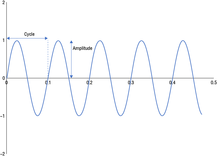
Photons are what actually carry all forms of electromagnetic energy, from microwaves to visible light to X-rays. Radio waves use electromagnetic energy, but a radio wave is fundamentally different than a wave on the ocean or a light wave. A radio wave has two components: frequency or wavelength and amplitude, often represented in a graph as shown in Figure 4.1. Frequency or wavelength is the measured change in electromagnetic energy within a specific time period called a cycle. In the following section I will explain that concept further.
Figure 4.1 Representation of radio wave at 10 Hz with an amplitude of 1
Without any context, you're likely to look at the diagram in Figure 4.1 and assume that this is what a radio wave looks like. It's too easy to walk away with the idea that a radio wave is like a rope jutting out from an antenna and bobbing about in a wavelike motion, slapping some distant receiver. Although this makes for a funny visual, the reality is a bit more sensible.
Frequency
Frequency is measured in Hertz (Hz), what used to be called cycles-per-second (cps). To simplify things, visualize a radio wave as a burst of a cloud of photons emanating from an antenna and moving outward at roughly the speed of light (the exact direction depends on the design of the antenna). Photons are carriers of electromagnetic energy, so you may also think of photons as simply energy if you prefer. Each burst of photons is a single wave. The number of waves that are emitted per second is called the frequency. The number of photons emitted in each burst is the amplitude.
Amplitude
The amplitude of a signal measures the power of a radio wave at a given point in space. The strength of a radio signal is proportional to the photon density. As the waves move farther from the transmitter, the amplitude decreases. A receiver standing right next to the transmitter will get hit with a lot more photons—and hence a lot more energy—than a receiver 10 miles away. The farther away you are, the fewer photons you can receive, and the weaker the signal will be. Signal strength decreases with distance.
You can visualize a radio wave as a flashing beacon light sitting atop a high tower. If the beacon flashes once every second, its frequency is 1 Hz. The brightness of the beacon is the amplitude. You could say that the beacon is a radio station transmitting at a certain frequency. If this sounds simple, it's because it really is. The complexity of radio waves comes into play when you use them to transmit data. More on that in a moment, but first, let's get a clearer handle on the significance of frequency.
Imagine you're viewing the beacon through dense fog at night. The brightness is such that you can barely make out the flashes, and you can't see the bulb or tower at all. Suddenly, the flashes start coming at a different frequency: twice every second. What happened? Here are a few possibilities:
The beacon increased its frequency to 2 Hz.
A pirate beacon appeared next to the first one and began operating at 1 Hz.
A pirate beacon appeared next to the first one and began operating at 2 Hz.
Or it could be a combination of these, such as both beacons flashing at 2 Hz in perfect sync. The same dilemma occurs with radio frequencies, and it's why in many cases laws forbid different radio stations from operating on the same or similar frequencies unless they're separated by a sufficient distance.
If it were the case that a pirate were operating a second beacon at the same 1 Hz frequency, we'd have a case of interference, and it would be impossible to distinguish the pirate beacon from the legitimate one. On the other hand, if you could reasonably assume that no pirate beacon was operating on the same frequency, then we'd know that our beacon simply increased its frequency to 2 Hz.
Radio waves don't come in different “colors” the way visible light does, so for the purposes of the analogy, the color of the beacon is irrelevant. But if you want to consider it, think of the color (let's say it's red) as the medium—that is, radio. A different color such as blue would be a different medium, such as a copper wire carrying an electrical current.
Carrier Frequency
Now that you understand how radio waves function, let's turn to how you use them to send information. The concept of carrier frequency is the foundation of all radio transmissions. Essentially, the carrier frequency is what carries data. Both the sender and the receiver must be tuned into the same carrier frequency to be able to communicate. To view it another way, the carrier frequency is a clocking mechanism that allows a receiver to stay in sync with the sender so that it's able to properly decode what the sender's sending. To illustrate how it works, we'll construct a scenario using the beacon analogy.
Imagine that you need to use a flashing beacon to transmit digital data. To keep things simple, let's assume the only symbols you need to transmit are 0 and 1. The first thing you must do is decide on a carrier frequency. Suppose you choose a carrier frequency of 2 Hz so that the beacon flashes twice every second when no data is being sent. To encode data using your beacon, you have two options; you can encode signals by modifying the frequency of the beacon or by modifying the brightness of it. These correspond to frequency modulation (FM) and amplitude modulation (AM), respectively.
Frequency Modulation (FM)
To encode data using FM, you could lower the frequency by 1 Hz to encode a 0, while increasing it by 1 Hz to encode a 1. Hence, a frequency of 3 Hz indicates a 1, and a frequency of 1 Hz indicates a 0.
Using this scheme, imagine that a receiver sees three flashes in a second (3 Hz), followed by a single flash a second later (1 Hz), and then two flashes every second thereafter (2 Hz). Because the receiver knows the carrier is 2 Hz, it simply compares the frequencies of the received signals to the carrier frequency and decodes the information accordingly. The received bits are 1 and 0, followed by no more data.
Notice that the throughput potential of this approach is quite limited. We can't transmit more than one bit per second. When used with digital data, frequency modulation is called frequency-shift keying (FSK).
There is another scheme called phase-shift keying (PSK). Both PSK and FSK modify the frequency of the carrier signal. You don't need to understand the subtle differences between PSK and FSK—just know that both are limited in terms of the amount of throughput they can achieve. In Wi-Fi networks, quadrature PSK (QPSK) is used as a fallback mechanism in environments with radio interference, but it can't support throughput rates much above 18 Mbps.
Amplitude Modulation (AM)
To encode data using AM, you can make use of different amplitudes. The amplitude is analogous to the beacon's brightness level. Suppose the beacon has three different brightness levels: low, medium, and high. We'll use a low brightness to encode a 0 and a high brightness to encode a 1. A flash of medium brightness indicates no data.
Suppose a receiver sees the beacon very bright for 1 second, dim the next second, and then bright the third second. The carrier frequency is 2 Hz, and the frequency of the beacon flashes doesn't change, so the receiver must interpret the amplitude at each cycle. Hence, the data received is 110011.
Something profound about amplitude modulation is that the achievable throughput is proportional to the carrier frequency. For instance, by raising the frequency to 100 MHz, it's possible to encode 100,000,000 bits per second (100 Mbps)!
It's also possible to combine modulation methods. Quadrature amplitude modulation (QAM) uses AM and PSK to achieve unbelievably high throughput. In fact, in Wi-Fi networks QAM is exclusively used to achieve speeds of 24 Mbps and up.
To see a beacon light through dense fog, it may be necessary to increase the amplitude or brightness. In the same way, in order for a radio signal to get where it needs to go, the transmitter must send it out with sufficient power to overcome distance, obstacles, and even radio interference. I briefly mentioned amplitude as a measurement of power. At a transmitter, amplitude is proportional to the number of photons (i.e., the amount of energy) emitted in a given cycle. But when it comes to radio, what really matters is the power of the signal at the receiver.
Power Levels
When we are dealing with large broadcast transmitters, radio transmission power is measured in watts (W). But the output power of Wi-Fi radios typically doesn't reach even 1 watt, so their power is measured in milliwatts (mW), or 1/1000 of a watt.
A typical Wi-Fi access point (AP) may have an output power of 100 mW. As the signal from the AP travels and encounters obstacles, its power will decrease. By the time it reaches a client, the signal strength may be 0.00001 mW! However, suppose the client moves a bit closer to the AP and now is receiving a signal strength of 0.0001 mW. That's better, but how much better? Is it worth moving the client permanently to a different location for an improvement of a fraction of a mW?
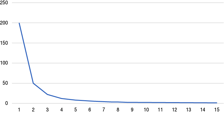
This leads us to an interesting discovery about radio waves (and all electromagnetic energy). You know the power of a signal decreases with distance, but it doesn't decrease linearly. If you consider that a radio wave is a cloud of photons radiating outward, like an expanding sphere, it's intuitive that as the sphere grows, the density of the photons—the amplitude—will decrease exponentially. To use another illustration, think of a balloon. As you inflate a balloon, the skin becomes thinner and thinner. In the same way, the amplitude or power density of a signal decreases with the square of the distance, as shown in Figure 4.2.
Figure 4.2 Amplitude decreases with the square of the distance.
This shape is called a power law distribution. If a station is close to the AP, any move closer or farther is going to make a dramatic difference in received signal strength. On the other hand, if a station is far from the AP, moving the client slightly closer is going to make only an infinitesimal difference.
Decibel (dB)
The decibel compares two different power levels and yields an absolute number that indicates the ratio between them. Decibels are useful for representing ratios that range from extremely large to very small, such as you might have when comparing power levels that vary by orders of magnitude. In radio, dB is often used to represent signal gain or loss. Let's use the earlier example with the tiny mW levels, plugging them into the following decibel formula:
A2 = 0.0001 mW
A1 = 0.00001 mW
dB = 10*log (A2/A1)
You want to compare the new and improved signal value (A2) against the original or reference value (A1). Plugging the values into the formula yields a value of 10 dB. Hence, you can say that moving the station resulted in an increase of 10 dB. See how this corresponds with the fact that A2 is 10 times the value of A1. This exemplifies one of the well-known decibel laws called the law of 10s, which states that every 10 dB indicates a tenfold difference between the numbers being compared. Suppose now you move the receiver closer to the AP and get a received mW power of 0.1 mW. This would yield a result of 40 dB, indicating that the new signal is 10,000 times as much as the reference signal!
The law of 3s states that every 3 dB difference indicates a twofold difference in the numbers being compared. This time we'll use a different example. Suppose a station has a received signal strength of 2 mW from an AP. The station moves closer and now has a received signal strength of 4 mW—a twofold increase. There isn't even a need to perform the dB calculation. Using the law of 3s, you can determine that the received signal strength increased by about 3 dB.
It's worth noting that dB values will be negative when the reference value is less than the given value. Using the last example, if the station with a 4 mW received signal strength moves away from the AP and winds up with a received signal strength of 0.8 mW, the difference is about –7 dB.
The closer the dB value gets to 0, the less of a difference there is between the compared signals. In cases of very tiny differences, it's possible to have fractional dB. And 0 dB indicates that the signals are the same, a fact aptly named the law of zeros.
Decibel-Milliwatt (DBm)
In most Wi-Fi networks you're not going to run into power levels much above a few watts, and even then only in environments like warehouses or large outdoor venues where an AP needs to crank out a lot of power to overcome dense obstacles or cover long distances. For the most part, you'll be dealing with milliwatts. The dBm measures power relative to a single milliwatt and simplifies dB calculations by assuming a 1 mW reference power. To see how to use dBm, consider a scenario where you want to find the signal loss between a 300 mW transmitter and a receiver. You'd start by calculating the dBm at the transmitter:
dBm = 10*log(300mW/1mW)
The power of the signal being transmitted is about 25 dBm. Now suppose that the signal strength at the receiver is 0.0000001 mW. Measured in dBm, the received signal level would be –70 dBm. With a little simple math, you can determine the net signal loss by subtracting the received signal level from the transmitted level:
25 dBm – –70 dBm = 95 dBm
The total signal loss is 95 dBm.
Antenna Types
Thus far we've focused on power from two perspectives: the power of a signal generated by a transmitter, and the power of a signal received by a receiver. But this is an oversimplification. There's another factor you now need to consider: antennas.
Antennas are the unsung heroes of radio. They're what radiate energy out into space and make radio transmission possible. You're not likely going to be designing your own antennas, so you don't need to understand the theory behind how they work, but you do need to know the different types of antennas used in Wi-Fi networks.
The isotropic antenna is a theoretical antenna that radiates energy in all directions equally. Even though it doesn't exist, it's used as a reference example of a perfect antenna against which we can measure our real antennas. Because it radiates equally in all directions, changing its orientation in space relative to the receiver won't provide any signal gain. Hence, we say that is has zero gain. Gain is a measurement of how much an antenna's radiation pattern favors a particular direction. With an isotropic antenna, a receiver can hover over the antenna, stand next to it, or sit below it, and as long as the distance from the antenna remains the same, the receiver will receive the same amount of power from the antenna. You measure antenna gain in terms of dB-isotropic (dBi), indicating the comparison to the perfect isotropic antenna. The higher the dBi, the more directional the radiation pattern. Gain can vary widely among antennas, even of the same type.
Omnidirectional antennas are what you think of when you hear the word “antenna.” Long, flimsy omnidirectional antennas are typically called whip antennas. Antennas like the ones you find on Wi-Fi radios are shorter, just a few inches in length, and are straight and rigid. Omnidirectional antennas radiate outward in a donut-like pattern. Just imagine placing a donut over the shaft of an antenna, and you have a good visual of the radiation pattern. The gain of omnidirectional antennas varies greatly. Antennas integrated into Wi-Fi radios typically have a gain of about 2 dBi, whereas external antennas may go up to 15 dBi.
Directional antennas concentrate the radiation pattern in a certain direction. The Yagi antenna, for example, is a type of directional antenna that forms an approximately 90-degree beam. This works nicely if you want to cover just one spot, such as an outdoor field. The parabolic dish antenna creates a tighter beam of about 10 degrees. Yagis have a typical gain of 10 to 15 dBi. Parabolic dishes are usually used on dedicated point-to-point wireless links such as those between two buildings or between a building and a tower. Parabolic antennas can have a gain of up to 30 dBi or higher.
Effective Isotropic Radiated Power (EIRP)
Although you typically don't see it, there's usually a cable connecting the transmitter and antenna. In the case of an external antenna, the cable can be quite long. The longer the cable, the more signal loss will occur, and such loss is measured in dB. The EIRP is the power measured in dBm radiated from an antenna after taking into account the transmitter power, cable loss, and antenna gain. For regulatory purposes, EIRP is the gold standard for measuring power output. In the United States, the maximum allowed EIRP for the 2.4 GHz band is 36 dBm, or 4 watts.
Suppose you have a transmitter generating a 12 dBm output. Its antenna cable has a cable loss of 3 dB, and its antenna has a gain of 5 dBi. For our scenario, the EIRP is calculated as follows:
EIRP = 12 dBm - 3 dB + 5 dBi
The EIRP would be 14 dBm.
Free Space Path Loss and Wavelength
As we've established, as a radio wave travels, it experiences a decrease in amplitude proportional to the square of the distance. I briefly mentioned that one reason for this is that the energy density of the wave spreads out thinner and thinner as it radiates outward, much like a puff of smoke becoming thinner as it dissipates. The distance affects what the amplitude of the signal is when it reaches a receiver's antenna.
The decrease with distance happens regardless of frequency. But as you move up into higher frequencies, the rate of amplitude decrease actually grows. This might seem surprising, since there's no intuitive reason a signal would weaken faster just because it's at a higher frequency. In fact, the reason for this latter phenomenon has to do with antenna lengths which are influenced by frequency!
To understand the significance of antenna lengths, you need to understand wavelengths. The wavelength (λ) of a signal is related to its frequency. Recall that frequency measures cycles per second. The formula for wavelength is given as
Wavelength = speed of light / frequency
You may see it written as λ = c/f, where λ is wavelength, c is the speed of light (m/s), and f is frequency (Hz). Wavelength is simply the distance a single radio wave travels during one cycle. For example, if an FM radio station is transmitting at 88.3 MHz, its transmitter is sending out a burst of energy 88,300,000 times every second! To calculate the wavelength, we'd do the following:
λ = (299,792,458 m/s) / 88,300,000 Hz
The wavelength is about 3.4 meters. That means when the transmitter sends a burst of energy, that energy will travel only about 3.4 meters before the next burst comes. Without getting into the physics, if an antenna is too long or too short relative to the wavelength, it won't radiate the signal as well. To maximize radiation, the length of the antenna should be the same as the wavelength. This isn't always practical, so half-wavelength or quarter-length wavelength antennas are often used.
The higher you get up into the frequencies, the shorter the antennas have to be. The wavelength for the 2.4 GHz frequency is about 5 inches. If you've got a 2.4 GHz AP nearby, measure the length of its antenna, and you'll find it to be pretty close to that. The 5 GHz frequency has a wavelength of about 2.36 inches, allowing for some rather short antennas! Higher frequencies mean shorter antennas.
Free space path loss measures the total signal loss as a function of increasing distance and frequency. The formula for calculating it is complex and you don't need to know it, but an example is instructive. Consider an AP and client 100 feet apart, transmitting at 2.4 GHz. The free space path loss between them is about 67 dB.
Now suppose you replace these devices with their 5 GHz counterparts. The free space path loss increases to 74 dB! The reason for the difference is that the increased frequency means decreased wavelength, which necessitates smaller antennas at the sender and receiver. Thankfully, you can easily overcome such losses by increasing the amplitude of the transmitting signal or using a higher gain antenna.
Free space path loss doesn't include amplitude loss due to encounters with obstacles or interference.
Received Signal Strength
The power of a particular signal received by a station, after making deductions for cable loss and antenna gain, is given by the received signal strength indicator (RSSI), which is measured in dBm. The RSSI ranges from –100 dBm to 0 dBm. A receiver can detect a signal down to its sensitivity level, which varies according to the way the radio is designed. Generally it's going to be closer to the –100 dBm end of the range.
All radio frequencies interfere with one another constantly. Ever present in any environment is a collection of random intertwined signals called noise. Noise consists of radio frequency (RF) energy from other stations, electrical wires, lightning, and even the sun. The sum of all these signals is called the noise floor. In order for a receiver to make out a signal, the RSSI must be greater than the noise floor. Both the signal amplitude and the noise floor can shift. For instance, if the noise floor is –80 dBm and the RSSI of a signal is –50 dBm, then the receiver can make out the signal just fine. A moment later, however, the signal may drop to –75 dBm, and the noise floor may increase to –70 dBm. Now the receiver can no longer pick out the signal among all the noise, even though it has actually received it.
Signal-to-Noise Ratio (SNR)
The difference between the RSSI and the noise floor is called the signal-to-noise ratio (SNR). Supposing the noise floor is –85 dBm and the RSSI is –50 dBm, the SNR would be
-50dBm - -85 dBm = 35 dBm
In order for the signal to be intelligible, the SNR must be greater than 0. A higher SNR is better. Another way of looking at it is that the greater the SNR, the more variation in signal loss and noise floor increase the receiver can tolerate and still be able to use the signal.
To hearken back to the beacon analogy one last time, imagine that you're looking at a flashing beacon in the dark of night. The SNR is extremely high since no other light is competing with the light from the beacon. Later, the sun rises just behind the beacon, overpowering its flashing strobe. The SNR in that situation is exceptionally low, possibly even zero, because the beacon is competing with the noise of too much ambient light.
WLAN 802.11 Standards
Now that you have a good understanding of radio theory, it's time to turn to using the airwaves to transport data. Just as IEEE 802.3 Ethernet defines the rules for wired networks of various flavors, the IEEE 802.11 family of standards defines the physical (layer 1) and data link (layer 2) standards for operation of WLANs.
The Physical Layer: Frequencies and Channels
You're no doubt aware of the various physical standards that the IEEE has put out over the years, dating from about 1999 to the present (2020). As of this writing, in order of earliest to latest they are
802.11a
802.11b
802.11g
802.11n
802.11ac
802.11ax
802.11n and 802.11ac are the most common today. Although the earlier standards are obsolete, you may still run into the occasional 802.11g network. You may wonder why there have been so many changes to 802.11 when Ethernet seems to have undergone relatively few. Both Ethernet and 802.11 have undergone layer 1 changes to take advantage of new technology in order to achieve faster speeds and longer range. In fact, 802.3 Ethernet has actually undergone more physical layer changes than 802.11.
The biggest difference between wired and wireless networks is the physical medium. It's obvious that wireless networks need different layer 1 standards to encode data as radio signals, rather than bits on a wire. Sounds simple enough. But compared to wired networking, wireless introduces two new distinct but related problems.
First, you can't change the physical medium. When you want to go from Gigabit Ethernet to 10 Gigabit Ethernet, you have to use a different physical medium that can support the new speed. In other words, you need new cables. But when it comes to wireless, you can't change the medium. Therefore, any improvements you make to wireless at layer 1 will have to be improvements in how you use the medium.
Second, with wireless, you're sharing the same airwaves with everyone else! Remember from Chapter 1, “Networking Fundamentals,” that the problem early Ethernet ran into was having too many devices sharing a single electrical bus. The solution was to break the medium up into separate collision domains. Clearly, you need a way to break up the wireless medium into separate collision domains. But unlike with an electrical bus, you can't just “disconnect” a portion of space from another, creating an impenetrable wall through which radio signals can't pass. You need a different approach.
The IEEE 802.11 layer 1 standards break up the airwaves into separate frequency ranges called channels. Devices that communicate on the same channel share a set of frequencies and are in the same collision domain. Ideally, devices in one channel should form a single collision domain and be isolated at layer 1 from devices on another channel. To use a crude analogy, devices in one channel are like workstations connected to an Ethernet hub.
Channels
A channel is a range of consecutive frequencies. The frequency range of each channel is its channel bandwidth (or just channel width). Bandwidth directly affects attainable data throughput because 802.11 simultaneously transmits on multiple frequencies at once. This approach is called spread spectrum because it multiplexes a single data stream over multiple frequencies. The more bandwidth is allocated to a channel, the more parallel data streams you can send. (Incidentally, this is precisely why the terms bandwidth and throughput are often used interchangeably.)
Different layer 1 802.11 standards allocate channels from different RF bands. The 802.11b/g/n standards all operate in the 2.4 GHz frequency band, whereas 802.11ac uses the 5 GHz band. These bands differ not only in their frequencies, but also in the way they allocate channel bandwidth.
The 2.4 GHz Band
The 2.4 GHz band is divided into 14 channels, each with a 20 MHz bandwidth, as listed in Table 4.1. If you look at the frequency ranges, you'll see that each channel has 22 MHz allocated but that only 20 MHz is actually used for each channel.
Notice that the frequencies of the channels overlap considerably. Each frequency represents a separate collision domain, so only one station at a time can talk on a given frequency. For example, channel 1 shares frequencies with channels 2, 3, 4, and 5. This means that adjacent channels can easily bleed into one another, defeating the whole purpose of channels to begin with. So why design it this way? The reasons were purely practical. When wireless networks were being dreamed up, there were other devices in the 2.4 GHz spectrum, and they didn't require more than 5 MHz of bandwidth. There's an old saying (usually falsely attributed to Bill Gates) that goes something like “640 KB of memory ought to be enough for anyone.” Well, the folks who came up with the 2.4 GHz band plan figured 5 MHz of bandwidth ought to be good enough for anyone. It was a reasonable assumption at the time.
Even in its early days, there wasn't a lot of room to work with. Today, not much has changed. Radio frequencies near the 2.4 GHz spectrum are used for mobile phones and industrial and scientific equipment. The 2.4 GHz band is crowded, and that's not going to change any time soon. The good news is that you can carefully select channels that don't have overlap. For example, if you're setting up three WLAN APs in an office, you can assign channels 1, 6, and 11 to avoid overlap. Of course, this works only if there aren't already any other wireless networks in the vicinity using nearby channels. The 2.4 GHz band is generally not a great place to be unless you're in a rural area.
The 5 GHz Band
IEEE 802.11n/ac makes use of the less crowded 5 GHz band. The exact frequencies of the 5 GHz band vary by country but range from 4910 to 5875 MHz. Unlike the straightforward numbering of the 2.4 GHz channels, the 5 GHz band is pretty convoluted. IEEE 802.11ac supports bandwidths of 20 MHz, 40 MHz, 80 MHz, and 160 MHz. But there are some strict limits for channel/bandwidth combinations, as shown in Table 4.2.
For bandwidths above 20 MHz, each channel consumes channels above and below it. For example, if you use channel 46 with a 40 MHz bandwidth, you'll be borrowing bandwidth from channels 44 and 48. To avoid using overlapping frequencies, your best bet is to use the same bandwidth for all your APs. That means if you want to make use of an 80 MHz bandwidth per channel, you have only six channels to choose from. Hence, if you need 25 APs at a site, you should stick with a 20 MHz bandwidth so as not to have any two APs competing on the same frequencies.
Dealing with Signal Degradation
If the signal degrades due to distance or interference, it's naturally going to introduce errors that will affect throughput and reliability. When an AP and client have a good connection, they'll use QAM to achieve high throughput. As the client moves away and the signal degrades, QAM doesn't work as well, and some packets may get dropped and have to be retransmitted, resulting in lower throughput. To compensate for this, they'll switch over to QPSK, which offers lower throughput but greater reliability.
Comparing 802.11 Physical Standards
You don't need to know the details of every 802.11 standard ever made, but you do need to understand the capabilities of the more modern standards. It goes without saying that an AP and client must use the same standard in order to interoperate. For example, a client that supports only 802.11g can't connect to an AP that supports only 802.11ac. Table 4.3 highlights key capabilities of each standard.
Table 4.3Comparing bandwidths and data rates of 802.11 standards
Standard
Supported band
Supported bandwidth (MHz)
Maximum data rate
802.11g
2.4
20
54 Mbps
802.11n
2.4, 5
20, 40
600 Mbps
802.11ac
5
20, 40, 80, 160
3.464 Gbps
802.11ax
2.4, 5
20, 40, 80, 160
9.6 Gbps
Layer 2: 802.11 Media Access Control (MAC)
Remember that OSI layer 2 sets up the rules for node-to-node communication within a subnet. You might guess that because both Ethernet and WLANs are standardized under the 802 family of standards, they provide a way for wired and wireless clients to interoperate with one another in the same subnet. And you'd be right! However, achieving that interoperability isn't as easy as you might expect.
Ethernet was originally designed for a shared medium—the thick yellow cable—so it would seem natural to just take the existing Ethernet standards and tweak them to apply to wireless networking. But surprisingly, this approach doesn't work. Ethernet uses MAC addresses to uniquely identify each node, and communication simply requires one node to address an Ethernet frame to another node. Notice that Ethernet takes it for granted that the two nodes are already physically connected to each other in some way. If you have devices connected at layer 1, the thinking goes, then they obviously should be able to communicate at layer 2. Devices that aren't physically connected just aren't part of the network. It's as simple as that.
But when it comes to wireless, these assumptions don't hold true. A wireless client isn't “connected at layer 1” in the same sense that a wired client is connected to a switch. Wireless clients can move in and out of range of an AP and each other. Furthermore, because the physical medium is everywhere and unrestricted, you have no control over whether someone blasts signals into your office or home. And radio is lossy and prone to interference, so data can get lost or corrupted easily. Let's look at how 802.11 overcomes these and other problems caused by using the lossy shared medium of radio.
Media Access
In a WLAN, accessing the medium really just means transmitting a radio signal. The distributed coordination function (DCF) is similar to Ethernet's CSMA/CD, except instead of sensing collisions, DCF attempts to avoid them. Thus, it takes what's called a CSMA/collision avoidance (CA) approach. DCF requires a station to wait for radio silence before transmitting. If the airwaves are busy, the station waits a random amount of time before trying again. There are other MAC methods, but DCF is the one that all 802.11 networks must support.
Authentication
Authentication mechanisms control which stations may establish an association with an AP, whereas encryption prevents data from being sniffed or modified in transit. Technically authentication and encryption are separate processes, but authentication and encryption often are used together. We'll cover encryption in a moment. The 802.11 family of standards offers the following authentication mechanisms:
Open System or Open Authentication This is practically the same as no authentication, and any station that requests it will be authenticated. Open systems don't provide any in-transit encryption. Public Wi-Fi hotspots almost always use this.
WebAuth WebAuth is a variant of open authentication that redirects users to a captive portal to complete some action before they're allowed to access network resources. See if this scenario sounds familiar: You go to a public hotspot and connect. You open your web browser and get redirected to a captive portal page that requires some action. It may prompt you to agree to some terms or it may ask you for a password or other credentials. After you enter the requested information and are authenticated, the system lets you browse the Internet. Since it's really just an open system, WebAuth doesn't include in-transit encryption.
Shared Key or Preshared Key A station must provide a password to associate with the AP. Shared-key authentication is almost exclusively used in conjunction with WPA personal mode encryption, which we'll cover in a moment.
802.1X This requires the connecting station (called the supplicant) to authenticate to an authentication server before it can join the WLAN. The authentication server can be the same one you use for other IT resources, such as a Kerberos or RADIUS server. IEEE 802.1X uses the Extensible Authentication Protocol (EAP) to integrate with a variety of authentication providers.
Association
The association process is how a station and AP negotiate the rules for communicating with one another. Association establishes layer 2 connectivity with the WLAN, and it can occur only after authentication is successful. When a station wants to associate with an access point, it sends an association request with the service set identifier (SSID) of the WLAN it wants to connect to as well as its supported data rates. The AP sends an association response with its own supported data rates. The station and AP can use the association frames to negotiate other options such as those related to flow control and encryption. Other options include performance and compatibility enhancements for the older 802.11 physical standards.
Encryption
In theory, radio signals can be picked up by anyone, so encrypting data sent over the air is the most significant thing you can do to secure a WLAN. Many open systems rely on encryption as a substitute for authentication. IEEE 802.11 offers three encryption mechanisms:
Wired Equivalent Privacy (WEP) Part of the original 802.11 specification, WEP was intended to mimic the privacy characteristics of a wired LAN. WEP uses the insecure RC4 cipher to encrypt data, but because it was incorrectly implemented, it's vulnerable to reverse-engineering the encryption key. It's been easily crackable for well over a decade. Never use it!
Wi-Fi Protected Access (WPA) with Temporal Key Integrity Protocol (TKIP) WPA-TKIP, also known as WPA1, was the answer to WEP's weaknesses. It also uses RC4 but implements it in a slightly more secure way than WEP. However, because it uses RC4, it's still vulnerable to exploits, so I recommend you don't use it. One reason WPA uses the computationally light RC4 cipher is so that older devices that support only WEP can be given WPA capability with a simple firmware upgrade.
WPA2 with CCMP WPA2 uses the AES cipher implemented using an encryption mechanism called CCMP (an acronym that has four different meanings depending on who you ask). The AES cipher is much more secure than RC4, and the CCMP implementation of cryptography is superior to TKIP. WPA2 much more computationally intensive than WEP and WPA1, but modern hardware is more than capable of handling it.
WPA3 with CCMP This is the latest iteration of WPA, and like WPA2, it uses AES and CCMP. But it adds some additional security for personal (preshared key) implementations. It also implements forward secrecy, which prevents an attacker from decrypting captured traffic even if they know the shared key.
Encryption isn't the same as authentication, but it does provide a way to control access to the WLAN. For example, if you enable WPA2 with a preshared key, users must type the key into their device to be able to connect. WPA used with a preshared key is called WPA personal mode. But this isn't the only option. Encryption can be used in conjunction with 802.1X authentication. When 802.1X and EAP are used in conjunction with WPA, it's called WPA enterprise mode. Once the user authenticates using whatever method you've allowed (user credentials, smartcard, certificate, one-time-password, etc.), their client and the AP will automatically negotiate WPA2 encryption without any further action on the user's part. This makes for a robust and seamless solution that provides authentication and encryption.
Error Control and Flow Control
The contention-based nature of wireless requires some coordination among transmitting stations. Unlike in a full-duplex Ethernet, Wi-Fi stations just blindly transmitting whenever they have data to send would result in radio interference and data errors. However, since there are few physical restrictions to the airwaves, radio interference is unavoidable. IEEE 802.11 provides flow control mechanisms to coordinate transmission and avoid errors, as well as error control features to detect and recover from data errors caused by interference.
Acknowledgments
In a way similar to TCP, 802.11 uses acknowledgments to indicate when a unicast frame is received. The sender marks each frame with a sequence number, and the receiving station responds with an ACK. If the sender doesn't receive an ACK to a frame, it will retransmit it. Retransmissions are usually the result of interference, obstacles, or insufficient signal strength. With the exception of a software bug or hardware error, retransmissions occur in only two cases:
The intended recipient never receives the frame, resulting in the sender retransmitting it.
The recipient receives the frame and sends an ACK, but the ACK doesn't make it back to the sender intact.
As you might expect, waiting for an ACK to a frame before transmitting the next frame slows things down quite a bit. To improve throughput, 802.11 offers the option of using block acknowledgments. Rather than waiting for an ACK to each frame, the sender sends a block of frames, and then waits for a single acknowledgment frame that indicates all the frames were received. You can think of this process as a two-way handshake. Unlike TCP's three-way handshake, there's no acknowledgment of the ACK itself.
Acknowledgments aren't sent for multicast frames.
Frame Check Sequence (FCS)
Radio interference has the propensity to corrupt data in transit, so all frames include a 32-bit checksum to aid in detecting corrupted frames. If a frame doesn't pass the FCS, it's silently discarded. If a sender receives a corrupted frame, it will not send an ACK in response. Likewise, if the sender receives a corrupted ACK frame, it will ignore it. Interference can cause data throughput to drop like a lead balloon!
Request-to-Send/Clear-to-Send (RTS/CTS)
RTS/CTS is an optional feature of 802.11 that helps avoid interference in cases where stations can't hear one another but can hear the AP. Therefore, these stations are more likely to transmit simultaneously, causing interference. Enabling RTS/CTS on these stations will cause them to defer to the AP before transmitting. When a station wants to transmit, it sends an RTS frame to the AP. The AP responds with a CTS that grants the station the privilege of transmitting for a short period of time. All other stations also receive the CTS and take note of the duration, so they know not to transmit during this window. This process dramatically reduces the potential for interference, although it's still possible for two stations to send RTS frames simultaneously. Note that enabling RTS/CTS in an environment where all stations can hear one another is unnecessary and will decrease throughput.
802.2 Logical Link Control (LLC)
In WLANs, layer 2 is actually divided into two sublayers: 802.11 MAC and 802.2 logical link control (LLC). This division is arbitrary and trivial but highlights another difference between 802.11 and Ethernet. The Type field of the 802.2 LLC frame serves the same function as the EtherType field in an Ethernet frame. The reason for using a separate LLC frame for this instead of just placing a Type field in the 802.11 frame is simply that IEEE has dictated that all 802 networks except Ethernet must use LLC.
Achieving High Throughput with Multiple-Input and Multiple-Output
Increasing transmit power and using complex modulation schemes can take us only so far when it comes to increasing data throughput rates. To get much over 100 Mbps, it's necessary to use multiple radios to create multiple simultaneous data streams. This method is called multiple-input and multiple-output (MIMO). There are two forms of MIMO:
Spatial Multiplexing The theory behind spatial multiplexing is simple: if you can push 50 Mbps using a single radio, you can push 100 Mbps by transmitting simultaneously using two radios on different frequencies. Spatial multiplexing takes the data to be sent, splits it up, and simultaneously transmits it using multiple radios. The receiver, of course, has to have multiple receiving radios and the capability to reassemble the separate signals into a single data stream. If a device has four radios for transmitting and two for receiving, then it's a 4×2 MIMO device. If a device has two radios for transmitting and two for receiving, it's a 2×2 MIMO device. 802.11n/ac/ax uses spatial multiplexing to achieve hundreds-of-megabits-per-second throughput.
Diversity The theory behind diversity is similar to that of spatial multiplexing, but with one small difference. One of the enemies of throughput is signal degradation. Diversity works by sending the same data simultaneously on different frequencies using antennas positioned differently. Because the signals are on different frequencies and take slightly different paths, there's a chance that one of them will encounter less interference or arrive at the receiver with greater strength. The receiver selects the best signal at any given moment, resulting in more consistent throughput.
Access Point Modes
An access point is a bridge between wireless clients and the wired LAN. Just as the area a switch can cover is limited by cable length restrictions, the area an AP can cover is limited by the RF environment and the AP's and clients’ capabilities. This leads to the need to deploy multiple APs to ensure coverage.
Cisco access points can operate in one of two modes: autonomous or lightweight. As the name suggests, in autonomous mode you configure each AP independently and it functions independently. This isn't so bad if you need to cover a small area, but if you have to cover a large campus, it becomes a management nightmare. To wrangle dozens or even hundreds of APs, you need a centralized management infrastructure. Thankfully, Cisco APs provide a lightweight mode, wherein the AP gives up its autonomy and relies on a wireless LAN controller (WLC) for its configuration and some of its functionality.
Autonomous
Autonomous APs are much like what you'd have at home, just a stand-alone AP that serves a small area. For the most part, autonomous mode APs work out of the box, acting as a bridge between a wireless client and a VLAN. Each AP functions as a self-contained unit, performing authentication, encryption, IP address assignment, traffic filtering, and 802.1Q tagging. If you need to cover just a small area with just a few APs, then autonomous mode might be right for you.
Autonomous mode is also ideal if you have wireless clients in the same area that need to communicate with one another. For example, wireless workstations may need to print to a wireless printer. By connecting all of them to the same AP and having them in the same VLAN, you ensure that traffic will flow through the AP without having to ever touch the wired network. This approach is particularly useful for small offices where there isn't a wired infrastructure.
But if you need to set up a larger collection of APs, autonomous mode can be cumbersome. You have to independently configure each AP and its connections to the wired LAN. If you want users to be able to seamlessly roam between autonomous APs, you'll have to trunk the same data VLAN to each AP. Extend a VLAN to a large number of APs and you'll wind up with a large, unwieldy broadcast domain, the potential for ugly bridging loops, and complex Spanning Tree topologies that may end up blocking ports you don't want blocked.
Lightweight
If you need more than 10 access points, you should consider the lightweight approach. In lightweight mode, an AP surrenders its autonomy and some of its functionality to a centralized WLC. The AP performs the physical layer functions of 802.11 and encryption, whereas the WLC controls the configuration of the AP and handles association and 802.1X authentication. This split-brain architecture is officially called the split-MAC architecture.
The WLC also terminates connections to the wired LAN, effectively acting as the LAN bridge for the AP. This lightweight approach greatly simplifies management and deployment of APs. Rather than trunking needed VLANs to each AP, you just trunk them to the WLC that APs use.
Each AP transports control and data traffic to and from the WLC via a dedicated Control and Provisioning of Wireless Access Points (CAPWAP) tunnel. Each AP needs only an IP address, which it can use to build a tunnel to a WLC. For the curious, the details of CAPWAP are codified in RFC 5415 (https://tools.ietf.org/rfc/rfc5415.txt).
A WLC can handle multiple APs, and because the CAPWAP tunnels terminate at layer 3, there's no need for the WLC and APs to be in the same VLAN. This tremendously improves scalability and makes it easy to centrally locate the WLC in a data center or wherever the network core happens to be. A disadvantage of the centralized approach is that if the WLC goes down or the AP loses connectivity to it, the AP ceases to function properly.
As an alternative to the centralized WLC, you can maintain a WLC in the same access layer as your APs. A simple way to do this is to use the Embedded Wireless Controller (EWC) functionality built into some Cisco switches and access points. This option represents a compromise between the autonomous and centralized topologies.
Wireless LAN Controller Selection Process
When you plug in a lightweight AP, it will attempt to automatically discover and set up a CAPWAP tunnel with a suitable WLC. Naturally, each AP needs a management IP address that you can configure manually. Otherwise, it will use DHCP to get one. After that, the discovery process begins.
WLC Discovery
Because APs in lightweight mode require a WLC to function, they have to pull out all the stops to make sure they're able to join a WLC. There are several methods they can use to locate a WLC.
To speed the discovery process, you can preconfigure an AP with the IP addresses of up to three controllers in order of priority—primary, secondary, and tertiary. You can alternatively configure DHCP option 43 on a DHCP server, populating the value with candidate WLC IP addresses.
Barring these two approaches, if the AP has never connected to a WLC before, it will broadcast a CAPWAP discovery request on UDP port 5246. Any WLCs that receive the broadcast will respond with a CAPWAP discovery response. On the other hand, if the AP has previously connected to one or more WLCs, it will have stored their IP addresses, and it will send the discovery request as a unicast to all of them.
Finally, just before giving up and starting over, the AP will try to resolve the domain name CISCO-CAPWAP-CONTROLLER.domain.local, where domain.local is the domain suffix learned from DHCP option 15. If it resolves to an IP address, the AP will assume it's for a WLC and will proceed to the selection stage.
The WLCs that respond with a discovery response compose the WLC candidate list that the AP will choose from in the selection process. When a WLC responds with a discovery response, it includes a metric indicating its current load. The load is a metric indicating the number of APs connected to it and how many total APs it can support. The AP will use the load information to determine which WLC to join.
Selection and Join
The AP sends a CAPWAP join request to the candidate WLC with the lowest load. This helps to ensure an even load distribution in environments with multiple WLCs. Once the WLC returns a join response, both the AP and WLC build an encrypted CAPWAP tunnel that they'll use for control and data traffic.
After joining, if the AP is running a software release that is different than the WLC, it will download the appropriate image from the WLC and reboot. After that, the AP will rejoin the WLC and download its configuration, which includes channel and authenticating settings and SSIDs.
If a WLC becomes unavailable or unresponsive after the AP joins, the AP can fall back to another one of the controllers in its candidate list. To improve availability, you can configure WLCs in a high-availability (HA) active-standby pair. If the active controller fails, by using stateful switchover (SSO) the standby controller can instantly take over.
Roaming and Location Services
By their nature, wireless clients don't tend to stay in one place. They roam around, often switching their association from one access point to another. In this section, we'll look at the different types of roaming, how they work, and how you can use data collected from APs to pinpoint the physical location of clients using location services.
Roaming
When a client senses that the signal from its associated AP is weak, it begins to look for another AP to associate with. It's up to the client to decide when to roam and which AP to associate with. Essentially, when a client roams, it disassociates from one AP and associates with a different one, so there is necessarily a temporary loss of connectivity. As long as 802.1X authentication isn't being used, roaming can occur quickly, in a matter of a few milliseconds. With 802.1X authentication, it takes closer to a second. The primary concern with roaming is not so much how quickly the client roams, but whether the APs and WLCs are configured to provide seamless WLAN connectivity to clients as they roam about.
Roaming between Autonomous APs
When using autonomous APs, you'll likely have them connected to a dedicated wireless VLAN. Using the power of transparent bridging, extending a subnet across all APs facilitates almost seamless roaming. When a client connected to one AP roams to another, it simply has to associate with the closer AP. It maintains its IP address, and as soon as it sends a frame, the switches update their MAC address tables accordingly to reflect the client's new location. Roaming just works, and it works even if there are several APs.
Roaming between Lightweight APs
In a lightweight topology, the functionality of each AP is shared between the AP and its connected WLC. As long as both APs are connected to the same controller, the roaming process works smoothly. This is called an intracontroller roam.
When a client roams between APs that are connected to different WLCs, it's called an intercontroller roam. This may occur when a client moves between buildings and associates with an AP on another controller. How clients roam between WLCs boils down to whether the WLCs share the same VLAN.
Layer 2 roaming—WLCs share a VLAN In layer 2 roaming, if both WLCs are connected to the same VLAN, the roam occurs similarly to how it does with autonomous APs. The client roams to a different AP, maintains its IP address, and the wired switching infrastructure updates its MAC address tables.
You'll notice that this scenario is not ideal from a design perspective. A single WLC can handle hundreds of APs, so you wouldn't likely have multiple WLCs except in a large environment. Extending a VLAN across such a huge network just isn't a good idea. Layer 2 roaming—like autonomous roaming—depends on the magic of transparent bridging. It works flawlessly until it doesn't.
Layer 3 roaming—WLCs don't share a VLAN The term “layer-3 roaming” is a bit misleading. It more accurately could be called “layer-2-over-layer-3 roaming.” If the WLCs are in different VLANs, they have to do a little behind-the-scenes magic. First, some terminology: The controller the client is roaming from is called the anchor controller. The one it's roaming to is the foreign controller. During a roam the foreign controller forms a CAPWAP tunnel with the anchor controller. All client traffic passes over the tunnel to the anchor controller, and the client keeps its original IP address. All that's really happening is that the foreign and anchor controllers are forwarding layer 2 traffic over layer 3. Using this process, the client can roam from controller to controller while maintaining layer 2 connectivity to its anchor controller.
Auto-Anchor Mobility
You may want to force certain clients to always go through a particular WLC regardless of the AP they're connected to. To use a common scenario, you may have an SSID for guest Internet access. You want this to be available everywhere, but you want all traffic to get routed through a firewall at your data center. You can achieve this by using auto-anchor mobility to force all guest clients to go through a WLC at your data center. Whenever a client connects to the guest SSID, regardless of what AP they hit, they will be automatically anchored to the WLC at the data center. This is also called guest tunneling.
Location Services
It may be desirable to know the location of wireless clients, be it for asset tracking, emergency services, just-in-time directions, or location-based advertising. The Location Services feature collects signal information from three or more APs and uses it to create a real-time map of Wi-Fi devices. You provide the physical location of your APs by placing them on a map, and Location Services uses a propagation model based on received signal strength to estimate the location of detected Wi-Fi devices. Location Services even works with devices that aren't associated with an AP. All Wi-Fi devices periodically send out probe requests to discover nearby APs, and all APs in earshot will receive these beacons.
Optionally, you can provide your own custom floor layout, making it easier to visually pinpoint a device's location. For greater accuracy, you can calibrate the model by placing a client in a specific location and picking out the location on the map. Location Services adjusts its model accordingly.
Cisco DNA Spaces provides cloud-based location services, and Cisco Connected Mobile Experiences (CMX) can be deployed on premises or in the cloud.
Summary
Wireless comes with more layer 1 and layer 2 scalability challenges than wired networks do. Today, 802.11 wireless standards and technology have matured to the point that with proper planning, wireless networks can be fast and reliable.
The 2.4 GHz band has been the standby for WLANs since the early 2000s. It's crowded, and that isn't likely to change soon. The 5 GHz band offers some breathing room, and especially if you're thinking of deploying wireless in a populated area, it's your best option for getting fast data speeds and avoiding interference.
Otherwise, when it comes to speed and reliability, the distance between your APs and clients is the most significant factor. Free space path loss and noise can be overcome by shrinking the distance between the transmitter and receiver. Hence, generally speaking, the larger your Wi-Fi environment, the more APs you'll need.
You may have noticed the conspicuous absence of any mention of wireless site surveys. These used to be popular tools in planning deployments when APs were so expensive that companies tried to achieve wireless coverage using as few of them as possible. But today site surveys are rarely necessary. APs are so inexpensive that there's no excuse not to have full coverage.
With a plethora of APs comes the problem of management. Wireless LAN controllers can push configuration to hundreds of APs, collect client location information, and facilitate rapid roaming between APs. WLCs can be integrated into switches or APs, so even when there's no robust wired infrastructure (such as in a small branch office), you can still enjoy the benefits of a centrally managed WLAN.
Exam Essentials
Understand when retransmissions occur. Retransmissions are usually the result of interference, obstacles, or insufficient signal strength. They have a profound impact on throughput and can result in the AP and client switching to a slower but more reliable modulation scheme. Reducing interference and increasing RSSI can keep you out of the woods.
Know the major differences between 802.11 standards. You don't need to know all the details, but knowing which standards use the 2.4 GHz and 5 GHz bands, as well as the top data throughput speeds of each standard, is important. Remember that 2.4 GHz and 5 GHz radios aren't compatible.
Understand the various authentication and encryption types. Authentication and encryption are different but are often used together. An open system has no encryption and may or may not use WebAuth for authentication. This is what you'll typically find in coffee shops. WPA Personal mode uses a preshared key for both authentication and encryption. WPA Enterprise mode uses 802.1X and EAP.
Be able to describe how roaming works in autonomous and lightweight deployments. Roaming is what sets wireless networks apart from wired networks. Clients are free to move about and expect the network to follow them, in a sense. Roaming is the client disassociating from one AP and associating with another using the same SSID. What matters is how the backend WLAN infrastructure handles this MAC move.
Understand the various antenna types. Omnidirectional antennas are the most common and have a relatively low gain. Directional or high-gain antennas are used to direct a signal toward a specific area. Directional antennas are most often used to connect two backhaul radios in a point-to-point fashion.
Review Questions
You can find the answers in the appendix.
What's the dB difference between 100 mW and 200 mW?
0 dB
3 dB
6 dB
10 dB
You have a station indicating a received signal strength of 80 mW. After moving away from the AP, the receiver indicates a loss of 6 dB. What is the new received strength in mW?
20 mW
40 mW
60 mW
74 mW
The power of a signal decreased by 10×. What is the dB of this change?
–100 dB
–10 dB
0 dB
10 dB
100 dB
A 100 mW signal increases by about 13 dB. What is the new approximate power level?
113 mW
1300 mW
2000 mW
2600 mW
A transmitter is emitting a signal with a power of 40 dBm. It's connected to an external antenna using a cable with a loss of 4 dB. The connected antenna has a gain of 12 dBi. What's the EIRP?
52 dBm
36 dBm
40 dB
48 dBm
Which of the following standards has the highest data rate?
802.11a
802.11g
802.11n
802.11ac
How might an access point respond when an 802.11 client's signal strength decreases?
Switch to a different channel
Reduce data throughput
Increase antenna gain
Initiate a roam
How many antennas does a 3×2 MIMO device have?
2
3
5
6
Which of the following is Open Authentication compatible with?
WPA
802.1X
Shared key
WebAuth
WPA2 enterprise mode uses which of the following? (Choose two.)
Preshared key
802.1X
WebAuth
EAP
A wireless client and a wireless printer are both connected to the same AP, which is operating in autonomous mode. The client and printer are in the same subnet. The AP is connected to a layer 3 switch. When the client prints to the printer, what path will traffic take?
Client → printer
Client → AP → printer
Client → AP → switch → AP → printer
None of these. Traffic can't flow between clients connected to the same AP.
How many CAPWAP tunnels are there between an AP and a WLC?
0
1
2
One per VLAN
What are two ways an AP can discover a WLC? (Choose two.)
Subnet broadcast on TCP port 5246
DHCP option 43
DNS query
Over-the-air broadcast
You want an AP to always use the WLC with the IP address 192.168.99.99. How can you achieve this?
Add 192.168.99.99 as a value for DHCP option 43.
Configure 192.168.99.99 as the primary WLC.
Create a DNS A record for the hostname CISCO-CAPWAP-CONTROLLER that resolves to 192.168.99.99.
Use a crossover cable to connect the AP to the WLC and boot the AP.
Using a subnet broadcast, an AP has discovered two WLCs: one embedded in a switch and another embedded in another AP. Which one will it attempt to build a CAPWAP tunnel with?
Both
It will select one at random.
The least loaded WLC
The one embedded in a switch
The one embedded in an AP
Which of the following always occurs when a client roams from one autonomous AP to another?
It associates with a different SSID.
It associates with a different AP.
It changes VLANs.
It disassociates from a WLC.
A client connected to a lightweight AP leaves a building and roams to another AP on a different WLC. Each building has its own subnet. The client keeps its IP address. Which of the following two things are true of this roam?
It's an intercontroller roam.
It's an intracontroller roam.
It's a layer 2 roam.
It's a layer 3 roam.
Which of the following does Location Services use to determine a wireless station's location?
RSSI
Cell tower triangulation
Gyrometers
WLC location
Noise floor level
Which of the following doesn't use a CAPWAP tunnel?
Layer 2 roaming
Intracontroller roaming
Autonomous mode
Lightweight mode
How can you force a client to always use a particular WLC regardless of what AP they connect to?
 There was a time when being a network engineer meant having to understand how data is converted into pulses of electrical current and carried along a wire. But thanks to the ubiquity of Ethernet standards, you don't need to think much about the physical medium of wired networks or how layer 1 interfaces with it. In wired networking, you can direct the signal where you need it. It's easy to imagine the mechanics of wired networks because you can see the medium connecting nodes together. You can easily explain twisted-pair cabling to a networking novice because they can touch it, manipulate it, and see where the signals are going simply by following the medium. This is because almost everyone's familiar with how electrical current behaves. You take it for granted that in order to charge your smartphone, you have to plug it into a charger. Likewise, you don't expect the remote control to work if it doesn't have batteries. Aside from these mundane examples, you may have even had some unpleasant close encounters with current, such as accidentally touching a conductor carrying alternating current and feeling an unpleasant buzz. All of these instances reinforce your understanding that electrical current—and hence data—follows the path of a conductor that you can see and touch.