4
Delivery Option: The Link Between Futures and Credit Derivatives
Credit derivatives, which began as a means of hedging the loan exposure of banks, have taken on a life of their own. Now they are used for many purposes for which they were not originally designed.
For example, some investors use derivatives to construct synthetic corporate bonds. As current convention has it, this is done with two instruments: a credit default swap (CDS) and an interest rate swap. The credit default swap is a contract in which one party sells default protection to another. The interest rate swap is a contract in which one party makes interest payments at a fixed rate and the other makes payments at a floating rate. One would create a basis trade by exchanging a corporate bond with a credit default swap bundled with an interest rate swap. If the credit default swap premium plus the interest rate swap yield are better than or equal to the yield on the underlying corporate bond, then exchanging the cash for the synthetic makes sense.
Assumptions Behind the Credit Default Swap Basis
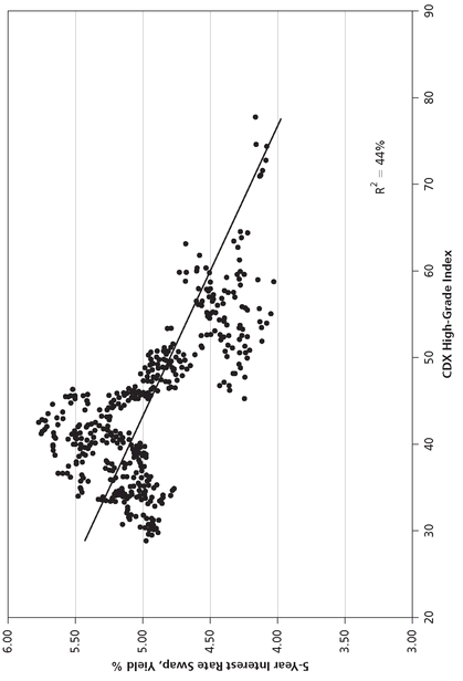
The important question to ask is: Should a credit default swap spread be added to an interest rate swap when constructing a synthetic corporate bond? When one does so, one assumes that the factors affecting credit spreads will not also affect interest rate swap spreads. In other words, the assumption is one of zero correlation. If this assumption is violated—in other words, if movements in credit spreads are correlated with movements in interest rate spreads—then the above construction offers far more risk than is present in the corporate bond. For example, if the credit swap has a spread DV01 (dollar value of 1 basis point) of $450 and the interest rate swap has an interest rate DV01 of $450, then the two better not be correlated, because if they are, the total risk of the position will be greater than $450 for every basis point change in rates. The corporate note in the cash market has a DV01 of only $450, so any correlation between credit spreads and swap rates adds unintended risk. Constructing a basis trade this way makes an interesting assumption about the correlation between the two derivative pieces, considering that one might imagine that an interest rate swap spread, the residual that’s left from receiving on an interest rate swap and selling a Treasury, is itself a credit spread. If it’s not a Treasury bond, there is a risk of default! However, the going assumption in the credit derivatives market is that the credit risks in interest rate swap spreads are independent of corporate default probabilities. How good is this assumption?
As Figure 4.1 illustrates, there are times when it isn’t realistic to assume independence between the derivative legs of a basis trade. Yield changes in a cash corporate note can be attributed to either a change in interest rates or a change in the probability that the bond’s issuer will default. Of course, both risk factors can change at the same time, but each influence can still be considered separately, because we can measure the price risk of a note by perturbing its yield by just one basis point. The same may not be true of credit default swap and interest rate swap spreads; there is evidence that during the period illustrated in Figure 4.1 there have been times when the two spreads have moved together. In this case, any positive correlation between the two would lead to a greater price risk in the synthetic bond than is present in the cash note. A true basis trade would swap identical risks to measure the pricing differences between each side. One can always make more money by taking more risk, but the point of constructing a basis trade is to take identical risks to discover pricing discrepancies. A first stab at arbitrage is to search for mispricings between risks that, by all rights, should be interchangeable. In order to adjust for correlation, one could measure the historical movement between the sides and then scale up or down the derivative pieces so that the statistical risk is comparable to the cash note. There are several problems with this approach. First, statistical measurements drift. Second, there is the problem of which side should be scaled—the credit or interest-rate swap? On the one hand, it is amazing that such a large market has grown up with such imperfect relative value approaches, but this might also be a testament to how sorely the credit market needed derivatives and how much utility they afford users.
Figure 4.1 CDX vs. Interest Rate Swap Spread
Source: Markit, Bloomberg
Default Probability, Corporate Debt, and the Delivery Option
Before digging into the mechanics of evaluating the delivery option, it is instructive to take a step back and consider the interactions we are studying. Accurately evaluating a credit default swap necessitates analyzing two markets: one for default probability and one for the debentures of the company. Rather than being divorced from the cash corporate market, credit derivatives are quite closely linked to this market through the structure of the embedded delivery option. The delivery option is a feature of trillions of dollars worth of outstanding credit derivatives. While the delivery option does have elements that behave like interest rate options, the triggers are very different. Interest rate options go in the money when there is a market move past a certain threshold. The delivery option goes in the money when a credit event occurs.
The cash flows of a credit default contract are influenced by changes in the probability that a particular company will default. Presumably, the higher the premium paid in the default swap, the more likely it is that a company will default or the greater the severity of that default will be. (The severity of default refers to the loss incurred by the protection seller after paying par for a note that may be worth less than par. Typically, one considers the probability of default and loss severity to move in lockstep, since it is relatively unusual for a company to be in financial distress but pose little risk of loss to its bondholders. The exception to this could be collateralized debt, a separate situation from evaluating the unsecured debentures of a company, which constitute the vast majority of credit default swaps.)
Even though default probabilities are the most important factors to consider when evaluating the cash flow of a default swap, it is also necessary to evaluate the structure of the market for the underlying debenture to determine the value of the delivery option.
Consider a default by a company with just one note outstanding: there is no delivery option since there are no alternatives for delivery except that one note. What if the company has two notes outstanding? The situation may or may not be very different than it is for the “one note” firm, depending on the differences between the two notes. For example, the two notes could be just three months apart in maturity, with the same coupon, in which case price movements would be nearly identical between the two. Although there is technically a choice about which note to deliver, the economic differences between the choices are relatively small.
But what if a company has two notes with a twenty-nine-year difference in maturities and the long bond is a zero-coupon issue? In this case there would be a great difference between the risks of the two issues, which would make the right to choose which note to deliver upon settlement of the contract quite valuable. Of course, companies rarely finance themselves with such a berserk barbell structure of discount notes and 30-year bonds. In fact, most firms have a fairly orderly structure to their liabilities. However, the point worth making is that the value of a delivery option is tied to the structure of the notes available in the cash bond market.
A Review of Treasury Futures Mechanics
In order to understand the interest rate options embedded in credit derivatives, it’s necessary to review the way this option works in Treasury futures.
A Treasury futures contract is not just an obligation to purchase or sell a single underlying note or bond on a specific date, but rather to purchase or sell a note chosen from a basket of underlying notes or bonds that will all mature within a predefined window. The size of the maturity window depends on the notional characteristics of the underlying futures contract. For example, the maturity windows for 2-, 5-, 10-, and 30-year Treasury futures are 3 months, 1 year, 2.5 years, and 15 years, respectively. In each case, the on-the-run issue in the basket has the most distant acceptable maturity date. As new bonds or notes are issued, they are automatically included in the basket; old issues fall out of the basket as they mature.
When settlement time comes, it is necessary to calculate how much the holder of the long contract will pay the holder of the short contract. Clearly, something must be done to account for the differences in maturity and yield of the various bonds that may be delivered to satisfy the contract. To solve this problem, the Treasury futures market developed a conversion factor system. Each issue that is acceptable for delivery is assigned a conversion factor, a value that is essentially a price for the bond using a 6 percent yield in order to even out differences in maturity and coupon. A conversion-factor system is a handful of things at once: a ratio of forward durations, the price at which the bond in question would yield 6 percent, and a common weighting for basis trades that spread a futures contract and cash issue against one another.
As an aside, there is an issue of semantics that old-time government bond traders instantly recognize, but which may not be obvious to the rest of the fixed-income world. A Treasury note is any coupon obligation whose original maturity is ten years or less when issued. A Treasury bond is an issue whose original maturity is longer than ten years, and is normally a thirty-year obligation. Of course, 30-year issues eventually mature, and there are many bonds with maturities of ten years or less, but in the Treasury market these issues are never considered “notes.” A bond is a bond and a note is a note, and a bond can’t ever become a note no matter the maturity. In fact, short-dated Treasury futures contracts are written in such a way as to allow for the delivery of any note within the delivery window, but since the contract specifies the word “note,” it excludes old 30-year issues that may fall within the window. In order to be technically correct when talking about the deliverable issues into Treasury futures, one must specify both “notes” and “bonds”—but since this is not a book about futures, from this point on we will cease to make the distinction.
Treasury futures expire each quarter, at which point the holders of short contracts have the right to choose which eligible issue they would like to deliver. The holders of long contracts are obligated to purchase this note if they hold the contract through the delivery date. By far, most contracts are offset prior to delivery, but as the notional value of Treasury futures grows, so does the number of notes delivered. If the holders of the short contracts (the people who have the option to choose which issue to deliver on settlement of the contract) are rational, they will choose to deliver the issue with the lowest price, referred to as the cheapest to deliver. When the notional value of contracts going through delivery outstrips the face value of the underlying notes or bonds, some of those holding short contracts will not be able to deliver cheapest-to-deliver bonds. As we’ll see, this is a risk found in both Treasury futures and credit derivatives.
Treasury contracts are written so that the holders of short contracts are long the delivery option. The short-contract holders have the right to purchase the eligible bond of their choice in the open market to deliver into the contract, but which note or bond is the right choice? It’s easy to look at the list of deliverable bonds to discern which issue has the lowest price today. But if interest rates were to change tomorrow, the bond with the distinction of being cheapest to deliver might also change.
Conveniently, there are two simple rules that guide the behavior of the bond that is cheapest to deliver:
1. . A steepening yield curve lengthens the maturity of the cheapest issue.
2. A bullish move in the market shortens the maturity of the cheapest issue.
When the yield curve steepens, the longer-maturity notes drop in price faster than the shorter-maturity notes because their yields are moving higher when nothing may be happening to yields on the front end of the curve. Higher yields mean lower prices: eventually the prices of those longer-maturity issues will fall enough that one of them will become the cheapest issue to deliver.
In a bullish move in the market, the shorter-maturity bonds rise in price more slowly than the longer-maturity bonds because they have lower durations. If rates move low enough, eventually the short-maturity bonds will have the lowest price in the basket, even if the yield curve moves in parallel.
The opposite is true for both types of curve moves as well: a bearish move in the market tends to move the cheapest issue to a longer maturity; when the yield curve flattens, the maturity of the cheapest to deliver becomes shorter.
It would be convenient if the yield curve either moved in parallel or by changing slope, but, as it turns out, the curve typically moves both ways simultaneously. Bear/flattening and bull/ steepening moves are the most common in the market. Typically the slope of the yield curve and the level of rates have been positively correlated. This positive correlation is sometimes referred to as a positive yield beta, indicating that the slope of the regression comparing the slope of the curve to the level of rates is positive. For futures traders, this correlation can be quite convenient, since each type of move offsets the other. For example, in a bear/flattening move the change in maturity of the cheapest issue is ambiguous: the bear move will drop the price of the longer-maturity issues, and the flattening will raise short-end yields and put downward pressure on those prices. The net effect is unclear and depends on the magnitude of each move. Conversely, there are combinations of yield curve and market movements that dramatically change the maturity of the cheapest issue, including bear/steepening and bull/flattening moves. In these curve movements, the change in maturity of the cheapest issue is unambiguous: it gets shorter in a bull/flattening move and longer in a bear/steepening one.
Traders live in fear of these kinds of moves. Those who have sold a delivery option are hoping against a switch in the cheapest issue, because a switch would mean that the option they have sold is in the money. Terrorism warnings ahead of long weekends and all manner of natural disasters make a delivery option seller break out into a cold sweat, because these kinds of news cause the types of yield curve movements that create the most pressure for the cheapest issue to change.
Pricing Treasury Futures Delivery Options
In a Treasury futures contract, there is a clearly defined basket of issues eligible for delivery, and the window of maturities of the issues in the basket widens with the maturity of the underlying note. For example, the window for 2-year-note futures is narrower than 5-year-note futures. The maturity for 10-year-note futures is wider still. Sometimes the cheapest note to deliver will be the one with a maturity at the very short end of the window. Other times, the cheapest note to deliver will be the one right at the end of the window. The cheapest-to-deliver note will change as the market and yield curve change. For example, if the cheapest issue to deliver is already the one with the shortest maturity in the basket, it can’t get any shorter in a bull move. If rates fall, the futures contract and cheapest note should perform nearly identically, because then there can’t be a switch to a shorter issue. Similarly, in an extremely high interest rate environment, the issue in the basket with the longest maturity will be the cheapest to deliver. Further moves higher in interest rates will not change the cheapest issue, and the futures contract and cheapest note should move in lockstep if rates continue to move higher.
There are a few observations worth making about these limiting cases. First, and most obviously, the delivery option is likely to have the greatest value when the cheapest-to-deliver issue is in the middle of the deliverables basket, rather than pinned to either the shortest or longest maturity. Second, the description of the behavior of the contract compared to the cash note sounds suspiciously conditional, like an option. It is not enough to say that the ability of the holder of short futures positions to choose which issue to deliver into the contract creates an option: one must be specific about the nature of that option in order to price it.
Suppose one considers only parallel moves in interest rates. When rates fall, the maturity of the cheapest issue decreases as well. Eventually yields will fall far enough that the issue in the basket with the shortest maturity will be the cheapest; no matter how much farther rates fall, there will not be an issue in the basket with a shorter term. Therefore, the cheapest issue will not change. Of course, if rates rise, then it is possible for the maturity of the cheapest issue to change in the opposite direction.
An option that goes in the money when rates rise and prices fall has all the basic components of a put. Similarly, as rates rise, the maturity of the cheapest issue will extend out along the yield curve; eventually the cheapest issue will also be the one in the basket with the longest maturity. As an aside, the issue with the longest maturity in each basket is the on-the-run note, which is typically quite rich because traders are willing to pay a premium for the liquidity it offers. For this reason, rates may have to move disproportionately higher to make the on-the-run issue the cheapest. If rates rise after the issue in the basket with the longest maturity is cheapest, there will not be a change in the cheapest issue. If rates fall, then the opposite will happen: an issue within the basket with a shorter maturity will become the cheapest issue. If one considers only parallel moves in rates, the delivery option can be perfectly replicated with a basket of naked options: puts to hedge against the risk of the cheapest issue moving to a longer maturity and calls to hedge against the risk of the cheapest issue moving to a shorter maturity.
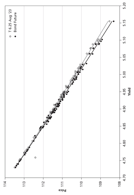
Figure 4.2 illustrates the situation by showing the relative performances of a bond futures contract compared to the current cheapest-to-deliver bond. As of the beginning of 2007, the shortest issue in the basket is cheapest. Therefore, the performance of the futures matches that of the cash bond when rates fall, moving left toward the y-axis. However, when rates rise, the performance of the futures begins to lag behind that of the cheapest issue, falling more dramatically than the price of the note in the bear market. It is not enough to describe in general terms how a futures contract with a delivery option will perform compared to the underlying cash note. Rather, the point of this exercise is to develop a framework for pricing the embedded option. If this fair-value methodology for valuing a delivery option is reasonable, then we can confidently compare our value with the market’s.
Figure 4.2 Empirical Perfomance of Treasury Bond Contracts Compared to Cheapest-to-Deliver issue
Source: Bloomberg, CBOT
The Fair-Value Method for Pricing an Embedded Option
The first step is to regraph the performances of the futures and cash bond in Figure 4.2 in terms of relative performance, using the cheapest-to-deliver issue as the baseline. See Figure 4.3. It is obvious from this chart exactly what needs to be added to the futures contract so that its performance matches the cash bond. The situation should be looking more and more familiar. This construction highlights exactly how the portfolio of put options should perform—as the mirror image of the futures’ underperformance.
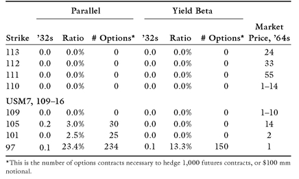
Suppose that we were to limit our portfolio of put options to exchange traded structures with expirations that don’t exactly match the expiration of the futures contract and with strikes that are listed at one-point increments. Given these limitations, it will be impossible to perfectly replicate the delivery option, unless all of the switches to the cheapest issue happen at yield levels that correspond to the strikes of the options we are using. Put another way, a delivery option can be viewed as a series of options whose strikes are the yield levels where switches to the cheapest issues occur. In the real world, the structure of a delivery option isn’t so well behaved. Even with this caveat, it is possible to come quite close to a perfect match with our basket of naked options, as illustrated in Figure 4.4. The dotted line represents the intrinsic value of various option strikes and how they might be combined in a portfolio. Given the pieces we have to work with, it is possible to find weightings of individual option strikes so that the performance of the overall portfolio matches the futures’ underperformance relative to the cash note. For credit derivatives traders, this may seem like an irrelevant exercise, but in fact these concepts are of supreme importance to valuing the delivery option in that market as well.
Figure 4.3 Long Bond Contract Perfomance Relative to Cheapest-to-Deliver Issue
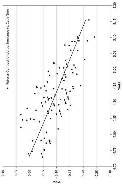
Table 4.1 Replicating the Options Portfolio for figure 4.3
An Option-Pricing Model
What may not be immediately obvious with this construction is what’s missing: an option-pricing model. How is it possible to value delivery option without an option-pricing model? Knowing the structure of the embedded option and how it is performing relative to cash, we can search for the amount of option protection we need among instruments that have observable market prices. The market prices delivery option via the individual component prices for the naked options. The final step to valuing delivery option is to multiply the weightings for each strike listed in Table 4.1 by the market price for each option. As the cheapest issue moves to ever-longer maturities, the underperformance of the cash bond grows. However, the options needed to hedge this risk are far out of the money and are relatively inexpensive, contributing little to the total value of delivery option. A great deal depends on our ability to measure the relative performances of the futures contract and the cash bond. This is where we start constructing a portfolio of options to offset the underperformance of the futures contract due to the embedded option. Of course, the fact that the person mak ing delivery has the right to choose a longer-maturity bond with the lowest price affects the price of the contract.
Figure 4.4 Principal Components Decomposition of 2-, 5-, 10-Year Treasury Note Curve into Primary Drivers of Volatility
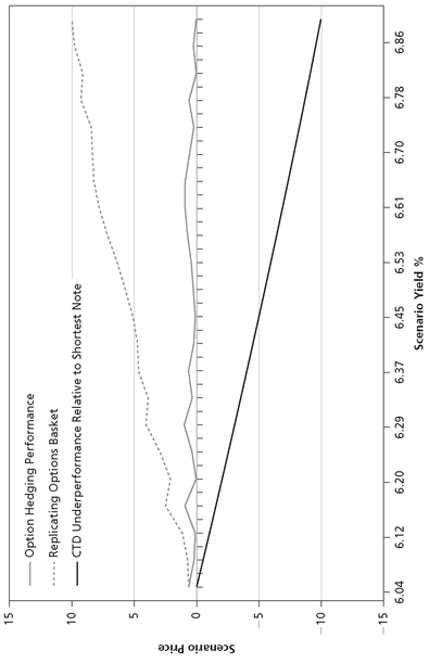
Before moving on to a framework for pricing a credit derivative’s delivery option, it’s worth noting that not all interest rate moves are parallel, and that the trigger events for credit and interest rate options are different. In the past, the level of rates and the slope of the curve have been correlated, making it unlikely that the strict assumption of parallel movement will hold.
Yield Beta
In order to compensate for this correlation between the level of rates and slope of the curve, one could adjust the yield movements (and reprice the deliverable bonds) so that the shorter issues in the basket move either more or less than the yield of the on-the-run note. For example, if the correlation coefficient is 1.2 for a 7-year note, one would say it has a positive yield beta, because every one basis point move in the on-the-run note (in this example, an issue with ten years to maturity) will move the 7-year note 1.2 basis points. Positive yield betas decrease the delivery option because the effects of level and slope movements partially offset one another. The yield-beta methodology, for which coefficients might come from historical observations, highlights how nonparallel curve movements may be incorporated into the same valuation framework.
Measuring the differences in the performances of the issues in the basket of bonds we’re interested in is still the hallmark of the analysis, and a yield-beta framework allows us to control the relative behavior of the bonds in a sophisticated way. Not only is it possible to amplify the yield movements of shorter issues with positive yield betas, but it is also possible to dampen their movements with negative yield betas, coefficients less than one for the shorter-maturity issues in the basket. As I mentioned before, bear/steepening and bull/flattening moves put the greatest pressure on the cheapest issue to change; negative yield betas cause exactly these types of movements. Yield betas are a convenient way of quantifying the behavior of the deliverables basket. Nonparallel rate moves will be revisited in the section on credit default swap delivery option valuation. (See Chapter 6.)
Cheapest to Deliver in Two Dimensions
The natural extension of this workis the creation of two-dimensional representation of the cheapest-to-defiver note that varies with changes in the level of rates and with the slope of the curve. With this two-dimensional representation, we can take into account nonparallel as well as parallel shifts and see the path of a positive or negative yield-beta move. Computationally, this extension is not much more complicated than the original work, except that we have to find a way to fairly shock the yield curve in nonparallel ways. The reason we have to qualify the exercise is that the yield curves of deliverable bonds are often quite complicated: the latest on-the-run issue commands a liquidity premium while the older issues tend to cheapen as they roll down the curve. Worse yet, specific issues—what would be called specials in the Treasury repo market—are sometimes in particularly high demand. These issues finance at particularly low and attractive rates for the holders of the bonds, and this attractiveness is reflected in the yield of the issue, because notes financing at attractive rates are usually bid up in price a little bit. The result is a yield curve that can be quite complex, with humps at all the usual points and even some idiosyncratic dips at popular maturities. How can we shock such an irregular curve?
The task is far easier in the government market, where regular issuance creates robust curves, and significant, multibillion-dollar face values tend to smooth out irregular demand for issues. One common method used to shock the curve in the government market is to first throw a line between the two on-the-run maturity points and to then drop a vertical line between the off-the-run issues and this imaginary line. As the slope of the on-the-run notes changes, the vertical distance between the off-the-run line and the interpolated line stays the same. The point is that every issue will change in yield by a different amount. For example, a 5-basis-point shock to the 2-year and 5-year slopes might result in a 3-basis-point move for an issue that is close to an on-the-run point, but still far enough away not to be subject to the whole move, perhaps a 3-year.
There is nothing particularly complicated about this, except for what happens when there is no active maturity point. Remember that in the corporate market, building a robust yield curve for a corporation’s liabilities is often not at the forefront of the thinking of a chief financial officer—unless that CFO happens to work at one of the handful of large issuers that come to market regularly. Why not just shock whatever notes are available ? For example, if a startup corporation had only 2-year and 8-year issues outstanding, why not just draw a line between the 2- and 8-year issues and call it a day? It’s certainly possible to shock any portion of the yield curve we please, but how could one company’s performance ever be compared to another’s?
A Standardized Method
The answer is that we need a standardized way to shock corporate curves, rather than relying on a catch-as-catch-can process of finding whatever issues are available. One relatively simple way to do this is to overlay the on-the-run Treasury yield curve on the corporate issuer we are interested in, and rework the process so that the vertical lines we draw from the outstanding issues drop to the interpolated Treasury curve, rather than to an interpolated corporate curve. Something that sounds as simple as creating an interpolated curve in the corporate market actually demands a great deal of care, because at any step along the way it’s possible to build in assumptions that come back to haunt us down the road. What if traders are looking for a delivery matrix and see that the delivery options in the default swap contracts they’re trading go in the money faster for corporation A than for corporation B? Heaven forbid they trade on that information only to find out that the scale between the two charts is wrong, and that what looks like a quick change in the cheapest-to-deliver issue is actually the original situation in reverse, corporation B facing a switch before corporation A. When conducting this type of analysis, it’s important to consider how the results could be used in the future. Armed with that foresight, we can avoid some pitfalls we might otherwise fall into.
That being said, the actual illustration is quite valuable to study. Once we have measured the basis-point spread between the corporate notes and the interpolated Treasury curve, we can begin to shock the Treasury points either in parallel or in various combinations of slope and level of yields. Suppose that we choose 5-basis-point increments for both the level and slope of the curve, so that our matrix will represent symmetrical moves in any direction. It should be obvious, according to the rules we outlined earlier, how the basket will behave from a general perspective: the maturity of the cheapest issue will lengthen when yields increase and shorten when yields fall. Additionally, the maturity of the cheapest issue will lengthen as the slope of the curve increases and shorten when the curve flattens. This leads to some more useful rules from a trading standpoint:
1. If the cheapest-to-deliver issue begins as the shortest issue in the basket then bull-flattening moves will keep it pegged as the cheapest issue.
2. For delivery option sellers (the sellers of protection in a default swap), the worst types of moves in the yield curve are bear/steepening moves, because they tend to move the back end of the curve more than the front end. This affects the longest-duration issues the most, dropping their prices precipitously compared to the prices of the issues at the front end of the curve.
There is a sequence of events that we have to understand in order to judge a delivery option’s performance. What if we determined that the value of the delivery option for a corporate issuer was 5 basis points, while the credit risk was worth 10 basis points? Then the default swap would be worth selling if it were priced at 20 basis points, a situation that implies the market is either pricing the credit risk of this contract incorrectly or that the delivery option is worth twice what we calculated as fair value. In this case we decide to sell protection and get paid the 20 basis points per year to accept the (hopefully overpriced) credit and delivery option risk.
This strategy is not without risk, because two things could happen: either the credit risk of the corporation we are interested in could deteriorate, or there could be a move in interest rates so that the issue we first imagined would be the cheapest to deliver is no longer so. Suppose that the delivery option seller, the seller of protection, seeks to hedge his or her risk by selling a note from the issuer short in the market with the same tenor, five years for both in this example. The synthetic long position should offset the performance of the short cash position, but what happens if there chances to be a 30-year note outstanding, and interest rates rise prior to a credit event? There are a lot of “supposes” and “ifs” in this statement, but imagine a situation where we wanted to unwind the trade, just prior to what seemed like an imminent default, without actually going through settlement. In this case we could be in quite a pickle, since the 30-year note would likely have dropped in price to be considered the new cheapest-to-deliver issue, and the synthetic side of our trade is probably going to follow the price of this note more closely than the original 5-year issue we sold short.
The problem here is that the note we sold short isn’t dropping in price enough to offset the losses on the synthetic long position (selling protection). If we hold the trade through delivery, then, weeks or months down the road, the two sides of the trade might hedge each other more effectively as all of the cash notes and synthetic trades begin to be priced at the expected recovery rate. Until that happens, the situation could be quite a mess as the mark-to-market wanders aimlessly. In this situation, interest rates have affected the synthetic valuation. Even if the recovery rate ends up giving us a higher price than the latest value for the 30-year note, the synthetic contract certainly won’t trade above the lowest-priced issue prior to settlement. The Delphi example in Chapter 7 illustrates this point.
..................Content has been hidden....................
You can't read the all page of ebook, please click here login for view all page.
