6
The Cheapest-to-Deliver Option in Credit Default Swaps
Default triggers physical delivery of a note in a single-name credit default swap. The foundation of the delivery option is that the buyers of protection have the right to decide which note to deliver, and presumably have paid a higher premium to gain that right. Typically, single-name credit default swaps are written so that any note from the issuer is deliverable as long as it has a maturity that is equal to or longer than the maturity of the swap, and the payment in exchange for the note is par. For example, if we create a default swap contract today that will expire in five years, and tomorrow the company we wrote the protection on defaults, then the protection buyers would need to purchase any note from the issuer so that they can then exchange it for par to the protection seller. Normally there is a thirty-day window for this transaction. How do we quantify this simple description into a price for delivery option?
Credit traders and analysts often say that when the prices of the defaulted notes are all the same, there is no delivery option. Wrong. This is only a half-truth. We can disprove it with a simple example based on the explanation of the delivery option in futures in Chapter 4. Before digging into the numbers, let’s consider what the common misperception refers to. After a corporation defaults, fails to make payment on a bond, restructures debt payments, or otherwise meets the International Swaps and Derivatives Association (ISDA) definition for default, it stands to reason that the debt of the issuer would trade at a substantial discount to face value. It has become typical to assume a 40 percent recovery rate in credit swap models, implying a 60 percent loss. An Enron bond that was worth $100 before the default may only be worth $40 after, but is every note of the issuer worth $40 the day before default, regardless of its maturity? It is the postdefault state that credit traders often refer to in their dismissal of the delivery option, rather than the time period from the day the contract is written until the day there is a default. The statement refers to a distribution of bond prices after there has been a default. Mixing in some truth is the easiest way to pass off a lie, and rather than doing the hard work of pricing the delivery option, traders often try to deny its existence.
While there is often a term structure of prices for defaulted notes, no simple assumption can explain it away, and one question makes it clear exactly why this is true: What happens to interest rates from the day the contract is written to the day a default happens? Remember, the contract calls for a par payment in exchange for any note from the issuer. For the moment let us restrict our analysis to a predefault world. If an issuer has two bonds, with maturities of five and six years, should it command more or less for the delivery option than an issuer that has bonds with maturities of five and thirty years? If interest rates fall, the 5-year note from each issuer will gain less in price than the 6-year note, given its shorter duration. Assuming that the coupons of all the issues are reasonably close, it will be the 5-year notes that will be delivered by each issuer. However, if interest rates rise it is a different story. In a rising interest-rate environment, the longer-maturity bond is going to lose value more quickly than the short-maturity bond. The 30-year bond is going to drop in price quite quickly because of its higher duration, and no matter the starting price or coupon of the 5-year note, its price will quickly be lower. It is the prerogative of the buyers of protection to choose a note to deliver in exchange for a par payment, and they should be willing to pay more for this choice when an issuer has a great deal of dispersion between the maturity of its debt compared to a firm with less of a maturity gap. Notice that we are still in a predefault world, and although we haven’t addressed the term structure of prices for defaulted notes, the value of the delivery option is obvious. There is some truth to the idea that all of the bonds of a defaulted company are admission tickets to the same show, the par payment by the default seller, and it makes sense to buy the least expensive ticket possible.
There are some corporations with 100-year bonds. The thought was to lock in low financing rates for a very long time, but obviously very little thought was given to how the structure of liabilities would impact the cost of trading credit protection in the derivatives market. Companies want an active credit derivatives market on their debt because it helps reduce borrowing costs whenever dealers or buyers can easily hedge their bonds. A corporate treasurer or chief financial officer would be shirking his or her responsibilities to create a debt distribution that cries out for higher default swap premiums. The untrained eye would read the higher premium as a sign that the market thought the company’s risk of default was higher than other companies’ risk, when in fact the differences merely have to do with the debt distribution and not with the credit risk of the company.
Credit default swap premiums translate directly to the costliness of debt in the cash market because of basis trades, in which the synthetic position is compared against the cash note in arbitrage trades. There is no escaping the feedback loop of derivatives on the cash market, and corporate officers need to be aware of the implications that their debt distribution has for the cost of their debt, not only through the term structure of rates but also through delivery option in default swaps.
Quantifying the Value of the Delivery Option
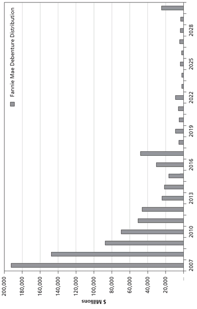
The first place to start in quantifying the value of the delivery option is with the distribution of debt for an issuer. Figure 6.1 illustrates the debt distribution for Fannie Mae, and it’s apparent that there is a wide range of maturities, from one to thirty years. In fact, there are over 5,000 individual notes, although most of them are from the medium-term note program and have face values of less than $100 million. To disprove the statement above regarding the value of delivery option for notes that all have the same price, let’s make a simplifying assumption regarding the issues in Figure 6.1, and suppose that all of the yields and coupons are the same, at 5 percent. Now the only thing that varies is the maturity and duration of the notes, with a DV01 of less than $100 per million to a maximum of $1,600 per million, meaning that every basis point in yield change moves the price of the note by this amount. Our initial starting point now matches every condition of the misguided adage regarding the price of delivery option: suppose the prices of all the notes from an issuer are the same. Remember that we start in a predefault world and we’re interested in the price of the admission ticket to receive the recovery rate for the defaulted issuer, whatever it may be.
Figure 6.1 Debt Distrubution for Fannie Mae
Source: Fannie Mae
Today the prices of all the deliverable issues are the same, since the coupon and yield are both 5 percent, but what about tomorrow? No one knows what will happen to interest rates over the life of the default swap, but it’s a safe bet that they will change. One way to describe this change is with an annualized yield volatility number. Credit default swaps are essentially options that pay off to the protection buyer in the event of a default; Black-Scholes would say that options decay at the square root of time. Yield volatility is the annual standard deviation of yield changes. It isn’t much of a stretch to suppose that the annual yield volatility of the corporate bonds in this example decays at the square root of time as well. In this case, a 10 percent yield volatility is worth 7.1 percent for half a year and 22 percent for five years. Since we’re looking at a 5-year default swap, the 10 percent annual volatility is 22 percent for five years. We already know that the yield of all the issues in the basket is 5 percent, so we can approximate that one standard deviation in yield change over the life of the default swap is 110 basis points. If the distribution is normal, then two standard deviations is 110 X 2 = 220 basis points. Now we know that however we evaluate the delivery option for the issuer we’re interested in, we have to evaluate the basket of deliverable notes from a range of 2.40 percent to 7.20 percent. The 10 percent yield volatility number we use here is completely arbitrary, but the mechanics would be the same no matter what volatility number we used.
A Proof by Contradiction
The most useful framework is a proof by contradiction.
We begin by approaching this problem as if the buyer of protection had no choice about which issue to deliver in the event of default—as if the delivery option did not exist. In a 5-year contract, for example, it would only be possible to deliver a 5-year note. It is easy enough to plot the price of a 5 percent note with a 5-year maturity over the range of yields in which we’re interested. These values will be our baseline performance for the credit default contract.
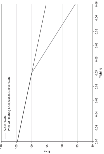
Now we can imagine a more realistic world: The buyer of protection has the choice of delivering not just a 5-year note but any note with a maturity that is longer than five years. In this example, with Fannie Mae bonds, there are issues with maturities all the way out to thirty years. Just as with a futures contract, the cheapest issue remains the shortest in the basket as interest rates fall. Since the duration of this bond is the lowest among the eligible notes, every other issue is going to rise in price faster than this one; the shortest issues remains cheapest for all parallel movements lower in interest rates. The interesting behavior happens when interest rates rise, as illustrated by Figure 6.2.
In our stylized example, every issue has the same price, so any increase in yields will drop the price of the longer-maturity issues faster than the price of the shorter-maturity issues. When rates rise, there is an immediate switch in the note that has the lowest price in the basket. All of the prices of deliverable bonds start out the same in this example, so the bond with the fastest price drop will immediately become the cheapest when rates rise. It will stay that way as rates continue to rise, moving from the shortest to the longest issue and skipping all of the intermediate maturities.
We now have two different series: Series 1, where the cheapest bond never changed, and Series 2, where we chose the bond with the lowest price in the basket to represent the performance of the contract. The second series is identical to the first in a lower rate environment, but its prices lag behind the first series as interest rates rise. We just proved with a simple exercise that the statement that assumes away the value of the delivery option is false, because the two series are not the same. Traders aren’t interested in proofs, although this example is illuminating; for them, the question is just what the delivery option is worth!
There is a little sleight of hand in our preceding analysis, because we never addressed the question of what time it was. All of the repricing of the deliverables basket in our example happened prior to default. What does that have to do with the prices of the notes after default? What if default does not immediately lead to bankruptcy? If an issuer is solvent, then it may still continue to operate after default. If this is the case, then its bonds continue to exist and will be priced to their original coupon and maturity characteristics in our example. Recently there has been research to suggest that default does not mean that the characteristics of the reference notes are irrelevant. For example, Guo, Jarrow, Zeng (2005) proposes a definition where default does not immediately lead to bankruptcy to model recovery rates for credit default swaps. Additionally, the settlement period for credit swaps is typically thirty days after a credit event. It is hard to believe that during that time the prices of 30-year and 2-year notes would remain fixed at their prices at the instant of default in the face of a month’s worth of changing interest rates. It isn’t too far a leap to think that the price of debt just prior to default impacts its postdefault price, and our admissions ticket analogy certainly holds for defaults that are anticipated. Even if the credit event were a complete surprise, the thirty-day settlement window and continuing-operations theory suggest a link between pre- and postdefault note prices. Recent history also provides some examples where default was anticipated and the buyers of protection had ample time to accumulate whichever note they wished from the market in anticipation of the par payment from the protection seller. For example, Delta and Northwest airlines both filed for Chapter 11 bankruptcy protection on Wednesday, September 14, 2005. Neither filing surprised the market. Delphi, a long-troubled auto parts supplier, filed for Chapter 11 on Saturday, October 8, 2005. Only traders who were asleep at the wheel had failed to notice the rising price of credit insurance, a reliable sign of imminent default, for all three companies. This reflects a scenario in which the delivery option behaves similarly to the way we have modeled it.
Figure 6.2 Performance of a 5-Year Note and a Delivery Option Basket with Thirty Years’ Worth of Maturities
Applying the Fair-Value Analysis
At this point, we can begin to borrow from our analysis of the futures market (see Chapter 4), since we need to reprice the deliverables basket according to the range of possible future yields. At each yield level we found the price of the cheapest issue and recorded this price along with our baseline price of a reference note. In order to extract meaning from these two columns of data, we have to compare them somehow, and the easiest way to begin is with a simple average of the two. The average price of the reference note, the 5-year note that we asserted would represent the performance of the credit swap if there were no delivery option, was par (Series 1). The average price of Series 2, where we allowed the cheapest issue to change, following whatever maturity had the lowest price, would be below par, since the longer duration issues would drop in price faster than the original note. The difference between these two prices is the empirical impact of the delivery option.
Still more work needs to be done to judge the price of this impact. If neither of the series we were interested in studying were convex, and the price moved 1:1 with the yield, then we might be able to stop at a simple average. The average price of the reference note isn’t exactly par, which was the starting price of the issue, because the price moved up by a little bit more than a linear estimate would predict in a rally and moved down by a little bit less in a sell-off. Ideally we could find a valuation approach that is not as heavily biased by the convexity of the issues involved, especially since it is the negative convexity of the delivery option that we are interested in studying!
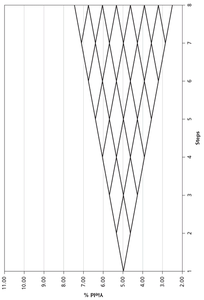
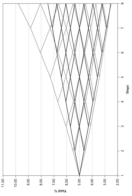
One alternative approach is to evaluate the two series of prices in a binomial tree. Figure 6.3 illustrates one possible construction of the tree, with equal yield changes at each point. Moving from left to right, one might imagine yields starting out at today’s value; over the eight steps we slice the coming five years into small pieces and allow rates to move higher or lower by the same amount in every period. Notice that the width of the binomial tree at the end of the five years matches the two-standard deviation calculation based on 10 percent yield volatility from earlier in the example. The binomial tree links today’s market to the possible future outcomes, but it does not discount prices in a meaningful way, as a present-value calculation would. We are simply interested in measuring the price impact that results from the fact that buyers of protection have a right to deliver any note they choose. First we consider Series 2, where we allowed the maturity of the cheapest issue to change. We know that all of the bonds in the deliverables basket started with a price of par, so is the difference between the simulated value in Series 2 and the par value of the delivery option? Is our job done?
Rethinking the Binomial Tree
We can be confident that we are getting closer to an answer we can be comfortable with, but there is an element of model-specification risk that should make most traders uncomfortable. Notice how easy it is to make assumptions regarding the specification of the binomial tree that have a major impact on the outcome of our model. Wall Street is full of dogmatic analysts who try to hide their shallow understanding of a topic by insisting a particular valuation method is the right one. The truth is that there are always alternatives and trade-offs when constructing a model. By their nature models are abstractions, in which compromises have to be made in order to simplify calculations—the alternative is the real world! The questions that should be asked are if the model is reasonable and if there are ways of using the model in a way that minimizes any bias that it might impose.
Figure 6.3 Example of a Binomial Tree with Equal Jumps at Each Increment
It may seem contradictory, but it is possible to use a model while still relying on it less. The way to do that is to evaluate our baseline series of a 5 percent 5-year note to see how far away from par the starting price is. This approach continues the proof-by-contradiction methodology. Whatever the valuation method, we are interested in first describing a world where the delivery option does not exist in order to measure its impact when we allow the buyers of protection to substitute the cheapest bond they choose. The initial price of our baseline series is still below the starting price of par because of the convexity of the issue, but it does give us an idea of how our valuation approach is leaving its fingerprints on the results.
One solution for evaluating our approach to valuing the delivery option is to compare the difference in initial prices using the binomial tree for each series. A trusting nature makes for a poor social scientist!
What could go wrong with our binomial tree approach, even if we are relying on the model as little as possible and only using it to search for differences in price between our two series? For one thing, binomial trees can be constructed differently. In this case we used a tree with equal jump sizes, but there are alternative specifications, the most important of which is to create a tree where the probabilities of moving higher or lower are the same but the basis-point changes from one period to the next are not the same. This second type of tree may be more realistic, since it accounts for greater yield changes from higher starting values and lower yield changes from lower starting values. For example, a 5 percent change from a 10 percent yield is going to lead to a 50-basis-point change, whereas a 5 percent change from a 2 percent yield will lead to a 10-basis-point change. Larger values create larger variances, even though the underlying process is often the same. Figure 6.4 illustrates how a binomial tree with equal probabilities is going to reach slightly higher yields than one with equal basis point changes. Evaluating our two series with an alternative construction of a binomial tree will serve as both a check on our original calculation and also a disquieting reminder of how dependent we are of the model for our answer.
Figure 6.4 Binomial Tree Built With Equal Probabilities
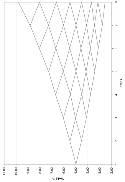
Imagine how the differing terminal values on the right-hand side of Figures 6.3 and 6.4 are going to impact the value of the delivery option. Figure 6.5 puts the two trees on the same scale. The tree with equal moves doesn’t reach as high in yield, which means that the longer-duration issues of the basket aren’t going to dip in prices as much as with the equal-probability tree. The difference highlights just how much our selection of a valuation method influences the results, because a subtle shift from a tree with equal jump sizes to one with equal probabilities impacts the value of our option even though we are simply using the trees to look at differences between our baseline series and the one where the maturity of the cheapest issue was allowed to change. There is another subtle distinction that we won’t bother to quantify, which has to do with the terminal values of each tree. The basis point change from the starting value to the top and bottom of the distribution on the right-hand side of the equal-jump-size tree in Figure 6.3 is different than the basis point change in Figure 6.4. Although we used the same series in each tree, the reality is that they imply different starting yield levels. Such subtlety should be frightening to anyone who is going to put money on the line. The basic problem that comes up over and over again with a closed-form-model approach is that we are not relying on market prices. Nowhere in this chapter have we used a market price. Although it might seem strange given the exercise we just completed, many recommendations by analysts do not rely on market prices, merely on the arbitrary choice of an approach that a particular person feels comfortable with. Both binomial trees are theoretically consistent and either would be a perfectly valid choice for a model, but how can we trade with data that builds from one abstraction to another? There is an alternative, and one that Treasury futures basis traders should feel right at home with.
Figure 6.5 Contrasting Two Binomial Tree Constructions
Market Pricing
Although credit default swaps are intended to hedge against default risk, the embedded delivery option lies firmly within the interest rate market. Rather than conjuring up some model to assign a value to the underperformance of the swap contract compared to the original cheapest issue, it is possible to mimic its performance with naked options that are priced by the market. The key is to establish a framework that lends itself to this type of market pricing. Before returning to our original example, let us make the distribution of deliverable bonds more realistic. Rather than assuming that all of the deliverable issues have the same coupon and yield, we can use the debt distribution from Fannie Mae, depicted in Figure 6.6, to craft a more realistic picture. While there are over 5,000 individual issues, we can aggregate the notes by year, taking the average price, coupon, and yield from actual data observable in the market. This represents a step closer to reality, but just this one step illustrates the problems inherent in using the actual data from an issuer. Admittedly, few firms have more individual issues and line items to contend with than the Agencies, and none of these calculations is difficult, but they are time consuming. Happily, computer power is inexhaustible.
It is interesting to note that the issue that would be the least expensive for buyers of protection is not the shortest in the basket, as we assumed with our earlier example of 5 percent coupon bonds, all with 5 percent yields. Should we use this issue as our benchmark? The alternative would be to choose a 5-year maturity note with a maturity matching the tenor of the contract. In theory, if we were to look at a world with no delivery, any note could be the reference security in a default contract, and there would be nothing restricting us to a maturity-matched note. For practical purposes, let us identify the current cheapest note as the one the buyers of protection would deliver in a default. Starting with a world where the delivery option does not exist, we evaluate the performance of the note with an annual yield volatility of 10 percent for a full five years, assuming that delivery option decays at the square root of time, as Black-Scholes tells us most other types of options do. The next step is to relax our assumption and once again grant the buyers of protection the right to choose the note with the lowest price to deliver into the contract at any given yield level.
Figure 6.6 Fannie Mae Debt Distribution With Yield Curve Overlaid
Source: Fannie, Bloomberg
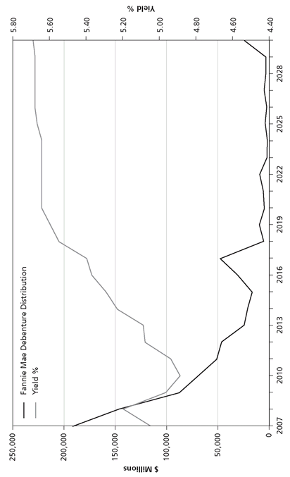
Figure 6.7 illustrates the performance of our two instruments. The first is the simple price and yield of the original cheapest-to-deliver (CTD) issue, and the second is the price of the lowest issue in the basket, moving to a 5-year note when rates fall and reaching all the way up to a 30-year note. This chart lists the performance of the two series outright, and the drooping performance of the default swap signals that the buyers of protection are choosing a different issue than the 5-year issue that was originally cheapest to deliver. Figure 6.8 depicts the same data, but this time it is compared against the cheapest issue. Of course, the price performance of the original cheapest to deliver has no difference with itself, and is shown in Figure 6.7. The underperformance of the contract also leaps out in this representation, and it’s clear that we have our work cut out for us to find some way to use market prices to measure this price difference. Just as in our work on Treasury futures, we can match a portfolio of naked options so that their payoff is a mirror image of the gap listed in these charts. What isn’t evident from these charts, however, is just how much longer the expiration of the options will need to be to span the entire life of the default swap.
Since the cheapest note in the basket is neither the shortest nor longest issue, both puts and calls are necessary to make up for the underperformance in bull and bear moves. We use options on 10-year futures, which are listed in one-point increments as a starting point, although these options are relatively short-lived and are only listed with a fixed set of strike prices. In order to determine the right ratio of the various strikes available, let’s set up the problem like a regression, minimizing the sum of squared residuals between our replicated options portfolio and the default swap underperformance relative to the original cheapest note. In this style of analysis, too much of a hedge is just as bad as too little, since we’re interested in the single portfolio with the best fit. Figure 6.9 illustrates the payoff from the replicated portfolio, the error introduced by limiting the strikes to one-point increments, and the ratio of each strike. The similarities between basis analyses for Treasury futures and credit default swaps basis are striking, and we can use all of the same tools we developed in the futures market with credit derivatives. Although all of the terminology is different, along with a few of the specifics on how to set up the problem, the economics of the two problems are the same.
Figure 6.7 Price and Yield ot the CTD Note vs. Lowest Issue
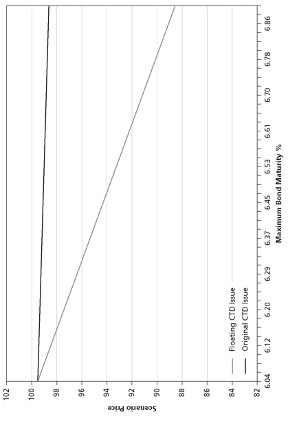
Figure 6.8 Underperformance of the CTD Compared to the Shortest Note Eligible for Delivery
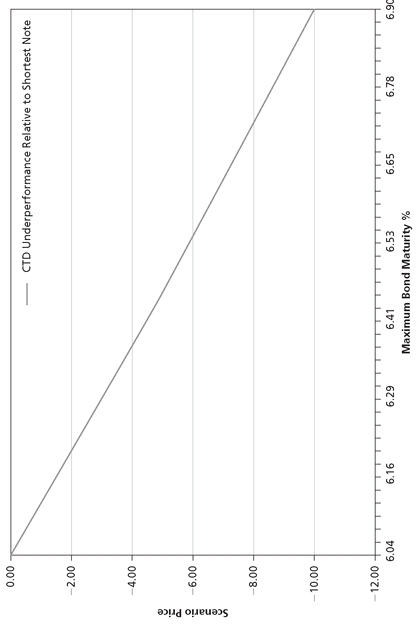
Figure 6.9 illustrates the resulting performance from our naked options hedge, restricting the strikes to one-point increments. The hedged portfolio, including the derivative with the embedded delivery option as well as the naked options, doesn’t result in a flawless hedge, as is evidenced by the somewhat wavy line along the x-axis in this chart. Unfortunately, there are switches to the cheapest issue that don’t happen exactly at the one-point increments our options are struck at, which means that there will be a small mismatch in performance. It might not be obvious at first, but we have created a powerful tool! The market prices each of the options, and the only way we have imposed ourselves on the analysis is by using a minimization routine to search for a portfolio with the minimum sum of squared errors compared to our target. Since the market prices these options, and we already know the ratios of each strike necessary to create our replicating basket, we simply have to multiply the two together to find the total value of the credit swap delivery option. Unlike in our work with the binomial trees, the market is pricing these options, and whether or not they are consistent with any formula, these prices are executable.
The options on the futures contracts we used in this example are relatively short-lived, but how does the analysis change if we use expirations that match the tenor of the contract? A 5-year option is going to be quite a bit more expensive than a 3-month option, but all of the mechanics are the same. In this case we use options on interest rate swaps because of the wide array of structures available. A 5-year option expiration would cover the whole life of the contract, but what should the underlying tenor of the note be? The longer the note the greater the convexity, and a 5-year note will struggle to keep up with the significant convexity of a 30-year bond. One approach would be to choose structures that match the tenor of the list of notes that are cheapest to deliver at various points in time. From Figure 6.6 it is obvious that some maturities from Fannie Mae will never be cheapest because of their price and coupon, and we can narrow the list of possible candidates this way. For purposes of illustration, we use a 7-year underlying note to mirror the earlier example using 10-year contracts, the cheapest-to-deliver note for which had a maturity of seven years.
Figure 6.9 Replicated Options Basket and Resulting Error of Combined Portfolio
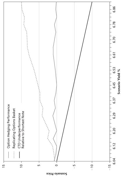
Recreating our analysis doesn’t yield significantly different results, although we do take another step to make the analysis realistic by relaxing our assumption concerning option strikes. Futures options on 10-year contracts have strikes at one-point increments, but over-the-counter instruments can have strikes anywhere. We allow the computer to search for strikes that best match the cheapest-to-deliver switch points. Remember that one way to think about the delivery option is as a series of naked options with strike prices matching the cheapest-to-deliver switch points. The results of this latest analysis are startling. The value of the delivery option jumped massively when we extended the expiration of the options from three months to five years. Part of this increase is to be expected, since time value alone can account for a large part of the difference. The balance has to do with the fact that we are using two distinct types of options in our analysis. Treasury futures options have relatively low-yielding Treasury notes as their underlying risk and have lower option premiums than higher-yielding interest rate swaps. Even if the expiration and tenor of the two options matched, it is likely that the Treasury futures options would have lower premiums, because they quite often boast lower yields and lower carry rates than the interest rate swap market.
Credit default swap traders might sense something rotten with the magnitude of these numbers, given that they are multiples of the current price for credit swaps on Fannie Mae. How can the delivery option be worth anything when Fannie Mae credit protection is trading at just a few basis points? The answer is that delivery option is only relevant when there is a default, and the entire value of this option isn’t applicable to the CDS premium. For Fannie Mae, a premium of a few basis points is quite low, indicating a low probability of a credit event, and so this low probability must be multiplied by our calculated delivery option value in order to determine the attribution between the credit and interest rate risk. Suppose that, using our earlier calculations, we come up with a probability of a credit event that is 10 percent. In this case, we take the $100 value of the delivery option and multiply it by 10 percent to discern the value of $10 per million. Have we concluded our analysis?
More Lessons from the Futures Market
This work has certainly taken us a long way toward an answer that we can base trades on, but there are a handful of lessons that have yet to be examined from the Treasury futures market that are instructive for a delivery in credit swaps. The first is that delivery is always discrete: no one will ever end up with a bond that represents the weighted average for a maturity, but rather a single issue will be handed from the protection buyers to the sellers in exchange for the par payment. Returning to our example with Treasury futures, there may be a cheapest note with a price of 100, while the second-cheapest issue has a price of 102. Should the buyers of contracts, who are obligated to pay for the notes, expect some amalgam with a weighted average price between 100 and 102? Not necessarily. If the long holders of contracts only take delivery of one contract, they will either receive the note worth 100 or 102, but there is no note with characteristics in between! If the buyers of contracts hold a large enough portfolio, then it is likely that they will receive some combination of the two notes, but deliveries are sometimes difficult animals to tame. In Treasury futures, deliveries are made by the vintage of the contracts, with the oldest long first in line for deliveries. Carry considerations sometimes mean that there are times when traders want to either get deliveries as late or as early in the month as possible, and there have been days when 95 percent of deliveries are allocated to a single trader who was not hoping for any notes. Even though the average delivery might happen in the middle of the month, the experience of individual traders may be nothing like the average. Translating this experience into credit swaps, we can infer that it is possible that not all of the deliveries will be made with a single issue, and there is indeed some evidence from recent credit events to support this conclusion.
Reference
X. Guo, R.A. Jarrow, Y. Zeng, “Modeling the Recovery Rate in a Reduced Form Model.” Working paper, September 15, 2005.
..................Content has been hidden....................
You can't read the all page of ebook, please click here login for view all page.
