
Appendix C
Computation of Partial Inductances
The computation of partial inductances represents a key component for almost all partial element equivalent circuit (PEEC) models, perhaps even more than the partial coefficients of potential in the following section. Many lower-frequency high-current problems can be solved with inductance-only models. Some references on this subject are [1–3] and also [4–7].
The evaluation of partial inductances Lp for the most general case involves the evaluation of a sixfold integral of the form (C.1) which is (5.15), or

where the details are given in Chapter 5.
The example formula (C.1) applies to the case where conductors 1 and 2 are bars or cells that are not necessarily parallel to each other. Obviously, for the partial self-inductances ![]() , the conductors 1 and 2 are the same. This case leads to a singularity if the points coincide such that
, the conductors 1 and 2 are the same. This case leads to a singularity if the points coincide such that ![]() . An advantage of an analytical solution for
. An advantage of an analytical solution for ![]() is that the singularity can be eliminated if two of the integrals for the same surface can be analytically evaluated.
is that the singularity can be eliminated if two of the integrals for the same surface can be analytically evaluated.
In general, we need to consider a larger class of configurations for the conductors or cells to cover all important cases. The evaluation of partial inductances for nonorthogonal structures is even more challenging. In the frequency domain for very high frequencies and sufficiently large cells, we may need to include the retardation in the integral that makes the analytical integration even more complicated. This issue is considered in Section 5.8.
The most simple and useful configurations are rectangular bars in a rectangular Manhattan-type coordinate system. As is evident from Chapters 5 and 7, it is much more challenging to find efficient formulas for the nonorthogonal case. Still, analytical formulas are very desirable for the larger aspect ratio dimensions that are often used in PEEC models. It is desirable to treat the largest physical dimensions of a cell analytically. This issue is considered in Appendix E. However, analytical solutions may also have limitations if the dimensions are too extreme as shown in Section 5.5.2. Fortunately, the use of double precision arithmetic used in most computers today is helpful for minimizing this problem.
In general, either analytical formulas are exclusively used or, alternatively, a combination of analytical formulas in conjunction with some numerical techniques are employed. This aspect is discussed in Appendix E.Key factors are sufficient accuracy as well as the reduction of compute time. Compute time is of importance since we may need to compute millions of Lp's for large problems.
Most analytical formulations for partial electrical element computations are for Manhattan-type rectangular geometries, which may be parallel to the ![]() axis and/or being parallel to the
axis and/or being parallel to the ![]() plane, where
plane, where ![]() is the origin. To be able to use the given analytical formula for many situations, it is necessary to rotate or shift the coordinate system so that the placement of the objects agrees with the orientation in the formula. For most situations, rotation and/or shifting is not necessary. We can reposition objects to the required location given by the formulas below in the
is the origin. To be able to use the given analytical formula for many situations, it is necessary to rotate or shift the coordinate system so that the placement of the objects agrees with the orientation in the formula. For most situations, rotation and/or shifting is not necessary. We can reposition objects to the required location given by the formulas below in the ![]() ,
, ![]() , and
, and ![]() coordinates.
coordinates.
We give the rotation matrices for all three cases, where a point ![]() in space is rotated about an axis to a new location
in space is rotated about an axis to a new location ![]() . Specifically, the rotation occurs about one axis by an angle the axis is left unchanged by the rotation. An example for the rotation about the
. Specifically, the rotation occurs about one axis by an angle the axis is left unchanged by the rotation. An example for the rotation about the ![]() -axis is given in Fig. C.1.
-axis is given in Fig. C.1.
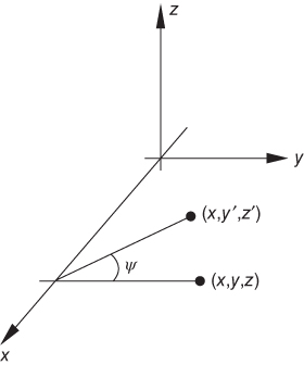
Figure C.1 Example of rotating a point by the angle  for
for  -axis.
The first case considered is the rotation about the ![]() -axis, which is illustrated in Fig. C.1. If the point is rotated by
-axis, which is illustrated in Fig. C.1. If the point is rotated by ![]() degrees, the point will be moved to
degrees, the point will be moved to ![]() from
from ![]() using the matrix
using the matrix

where ![]() .
.
The coordinates are rotated around the ![]() -axis by the angle
-axis by the angle ![]() to the new location
to the new location ![]() using
using

where ![]() .
.
Finally, if the coordinate is rotated around the ![]() -axis for
-axis for ![]() degrees, the rotated coordinates
degrees, the rotated coordinates ![]() can be obtained from
can be obtained from ![]()

where ![]() . In general, by combining these three steps, we can rotate the coordinates to align with any point in the coordinate system.
. In general, by combining these three steps, we can rotate the coordinates to align with any point in the coordinate system.
The situation is much simpler for the case where we have to shift a point in space in the coordinate direction. We simply add a constant ![]() in the appropriate direction. For example, we shift a point by
in the appropriate direction. For example, we shift a point by ![]() to new point by simply adding the changes, or
to new point by simply adding the changes, or

The above rotation and the shifting operations together allow changes to be made for the general case. Hence, it can be used for any one of the formulas given below.
To reorient the rectangular coordinate system, we simply exchange the coordinates in a cyclic way. An example is ![]() ,
, ![]() , and
, and ![]() . The issue is more complicated for the nonorthogonal formulas since we also may require to perform translations.
. The issue is more complicated for the nonorthogonal formulas since we also may require to perform translations.
C.1 Partial Inductance Formulas for Orthogonal Geometries
This appendix lists important formulas for the computation of the orthogonal partial inductance values. First, we want to repeat that partial inductance with orthogonal currents do not couple. This results in ![]() .
.
For clarity, we present all the formulas in the same coordinate system. Some of the formulas may need numerical solutions while others are analytically exact and are complete. Approximate formulas may not be accurate enough for some applications such as skin-effect computations like the volume filament (VFI) model in Chapter 9, where the cells are closely located. For these applications, at least 4–5 digits of accuracy is required. We should be aware that some of the approximate formulas in Ref. [1] have limited accuracy.
For several analytical formulas in this appendices we include very small numbers in the order of ![]() to
to ![]() to avoid possible artificial singularities for some combinations of input parameters. This is a conventional numerical technique to avoid singularity problems.
to avoid possible artificial singularities for some combinations of input parameters. This is a conventional numerical technique to avoid singularity problems.
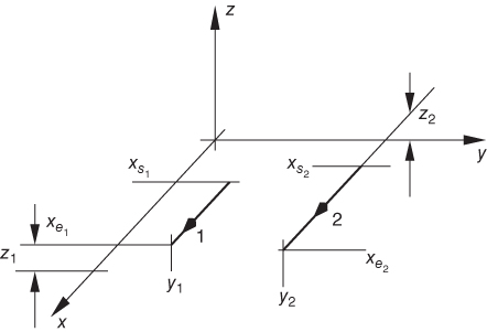
Figure C.2 Partial mutual inductance for two filament wires.
C.1.1  for Two Parallel Filaments
A simple important geometry is the wire-to-wire or filament-to-filament problem shown in Fig. C.2. Of course, the result is singular if the wires coincide. Filaments are very important building blocks, which we use for the combined analytical and numerical integration. The current direction in the wires is shown to be along the length.
The partial inductance formula for ![]() for two current filaments shown in Fig. C.2 reduces to
for two current filaments shown in Fig. C.2 reduces to

where
The analytical form of the partial inductance is given for this case by a simple integration step as

with
Note that ![]() represents the end of the object and
represents the end of the object and ![]() is used for the start.
is used for the start.
Equation (C.8) can also be used as an approximation to the round wire partial inductance especially if the wire diameter is small compared to the spacing. Of course, other cross section can be approximated efficiently with several filaments and numerical integration in the cross-section direction.
C.1.2  for Round Wire
We give two formulas for the partial self-inductance for round shapes. The popular equation for the partial self-inductance for the section of round wire shown in Fig. C.3 is

where ![]() is the usual distance between the source and observation points.
is the usual distance between the source and observation points. ![]() and
and ![]() are the cross sections.
are the cross sections.

Figure C.3 Partial self-inductance for round wire section.
The first formula is a simple approximation of a wire partial self- inductance used in Refs [1, 2], which is based on the assumption that the above filament formula can be used to represent a round wire by placing one of the filaments at the center of the wire, and the second one on the surface of the wire at distance ![]() away. The approximate result for this case is
away. The approximate result for this case is

where ![]() is the length of the segment. We could view this approximation technique as the most simple case of numerical integration based on the analytical result for the longitudinal direction.
is the length of the segment. We could view this approximation technique as the most simple case of numerical integration based on the analytical result for the longitudinal direction.
A second analytical formula is for the partial inductance of a zero thickness cylindrical tube with a radius ![]() shown in Fig. C.3. The integrals to evaluate are
shown in Fig. C.3. The integrals to evaluate are

by recognizing that symmetry can be used to reduce the fourfold integral to the threefold integral. We were able to analytically solve the integrals for the case of interest where the length ![]() of the wire is longer than the diameter
of the wire is longer than the diameter ![]() [8]. The result for the tube conductor is given by
[8]. The result for the tube conductor is given by

where ![]() . We should note that the equation is also used in equation (9.29) for skin-effect models [9].
. We should note that the equation is also used in equation (9.29) for skin-effect models [9].
C.1.3  for Filament and Current Sheet
Another important partial mutual inductance represents the case where one conductor is approximated with a filament and the other with a zero thickness sheet as shown in Fig. C.4. Of course, the current in the sheet is in the same ![]() -direction as in the wire as is shown in Fig. C.4 and the integral is given by
-direction as in the wire as is shown in Fig. C.4 and the integral is given by


Figure C.4 Exact partial mutual inductance for filament and sheet.
The analytical solution for the above integrals is

with
This formula is useful for the case where the two conductors are of a different shape. Other conductor shapes can be taken into account by combining this formula with numerical integration for the cross-section dimension of one or both inductive cells.
C.1.4  for Rectangular Zero Thickness Current Sheet
Fortunately, the analytical ![]() for a zero thickness rectangular sheet shown in Fig. C.5 leads to a relatively simple formula.
for a zero thickness rectangular sheet shown in Fig. C.5 leads to a relatively simple formula.
Figure C.5 Single zero thickness conductor sheets.
The result is

where ![]() and
and ![]() .
.
We note that this relatively simple formula is very useful for semianalytical solutions in layered models. Importantly, it eliminates the singular behavior problem for the partial self-inductance.
C.1.5  for Two Parallel Zero Thickness Current Sheets
Two zero thickness parallel current sheets are shown in Fig. C.6. Fortunately, several analytical formulas are available, for example, Ref. [2]. The integral to be solved is

The closed solution of integral (C.25) is

where
where we added ![]() to the equation as a very small number.
to the equation as a very small number.
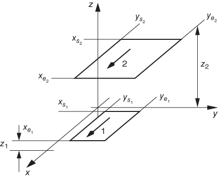
Figure C.6 Two parallel zero thickness conductors example.
C.1.6  for Two Orthogonal Rectangular Current Sheets
As is shown in Fig. C.7, two zero thickness sheets are at an angle of ![]() while the current flow is in the
while the current flow is in the ![]() -direction for both sheets. This formula is again very useful. Of course, the currents in the sheets as indicated in Fig. C.7 need to be parallel to each other for a nonzero partial inductance.
-direction for both sheets. This formula is again very useful. Of course, the currents in the sheets as indicated in Fig. C.7 need to be parallel to each other for a nonzero partial inductance.

Figure C.7 Two zero thickness conductors at a  angle.
Its original definition is

where the final result for ![]() for the two orthogonal current sheets is
for the two orthogonal current sheets is

with
and
C.1.7  for Rectangular Finite Thickness Bar
The partial self-inductance of a rectangular bar shown in Fig. C.8 represents an important building block for many problems. The equation for this case is given by

where the cross-section area is given by ![]() and
and ![]() and
and ![]() . The solution of this sixfold integral is in general obtained by introducing new variable differences for
. The solution of this sixfold integral is in general obtained by introducing new variable differences for ![]() . The closed form expression [4] is
. The closed form expression [4] is

with

and

The evaluation of (C.36) should for accuracy reasons be performed by summing from top to bottom, where the new terms are added to the sum of the previous terms. Test results show that the errors become large for very large values of ![]() and for small values of
and for small values of ![]() as considered in Section 5.5.2.
as considered in Section 5.5.2.

Figure C.8  for rectangular bar with thickness.
A possible solution for this is the computation of ![]() by breaking the length into several segments as is illustrated in Section 5.6.1. This is required only for very long conductors.
by breaking the length into several segments as is illustrated in Section 5.6.1. This is required only for very long conductors.
The accuracy problem for this case has also been observed in Ref. [10]. It is also pointed out that neighboring partial mutual inductances can be computed by using only partial self-inductance computations. Two neighboring block cells are shown in Fig. C.9. The partial self-inductance of the two neighbors cells shown can be computed using formula (C.36).

Figure C.9 Partial inductance for two rectangular conductors.
If we also compute the partial self-![]() for a combined block 1,2, then the result is
for a combined block 1,2, then the result is
Hence, we can compute ![]() totally based on partial self- inductance only, or
totally based on partial self- inductance only, or
This can be very helpful for skin-effect models where the accuracy is an issue due to the closely located neighbors. Hence, three partial self-inductance computations are required. This helps, since we can more accurately compute a partial mutual inductance ![]() for some geometries. We want to point out that this technique can also be applied to conductors in parallel as shown in Fig. C.9 (b). We leave the computation of
for some geometries. We want to point out that this technique can also be applied to conductors in parallel as shown in Fig. C.9 (b). We leave the computation of ![]() as an exercise to the reader.
as an exercise to the reader.
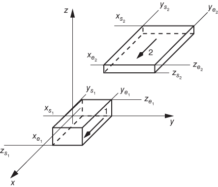
Figure C.10 Partial inductance for two rectangular conductors.
C.1.8  for Two Rectangular Parallel Bars
An important structure for rectangular PEEC models is the case of two parallel rectangular bars as is shown in Fig. C.10. The analytical formula for the mutual inductance between two rectangular bars is given in Ref. [3]. In our coordinate system setup, the formula is

with
and
We added this formula for completeness. Unfortunately, even using double precision arithmetic leads only to limited accuracy for reasonably large parameters in this formulation. For this reason, using thin layer approximations in Section C.1.5 with numerical integration along the thickness leads to more stable results.
C.1.9  Kernel Integral for Parallel Rectangular Sheets
Partial elements are of importance for other formulation such as the ones in Chapter 11 so that other material properties can be taken into account. In some of these formulations, integrals with a higher order Green's function need to be solved. Specifically, the integral for a ![]() kernel is important. Here, we consider the geometry to be two rectangles shown in Fig. C.11.
kernel is important. Here, we consider the geometry to be two rectangles shown in Fig. C.11.

where, ![]() .
.

Figure C.11 Zero thickness conductors example.
Then the final formulation of ![]() for two orthogonal current sheets is
for two orthogonal current sheets is

where the subscripts are for
C.1.10  Kernel Integral for Orthogonal Rectangular Sheets
A second important integral with a ![]() Green's function is for two orthogonal rectangles shown in Fig. C.12. For this case, we want to give a solution for the following integral
Green's function is for two orthogonal rectangles shown in Fig. C.12. For this case, we want to give a solution for the following integral

where, ![]() .
.

Figure C.12 Two parallel zero thickness conductors.
Then the final mutual high order coupling formulation ![]() for two orthogonal current sheets is
for two orthogonal current sheets is

where the subscripts are for
And
C.2 Partial Inductance Formulas for Nonorthogonal Geometries
This section is dedicated to the computation of nonorthogonal partial inductance values.
The general integrals for the computation of partial inductance for nonorthogonal such as nonorthogonal hexahedral elements are derived in Chapter 7, equation (7.18) as

It is clear that analytical solutions are even more challenging for nonorthogonal geometries. Still, analytical integration needs to be used as much as possible, especially for the longer dimensions of the cells. Since many problems are in this class, we want to efficiently solve problems with relatively long cells such as a thin wire-type structure. To accomplish this, we pursue a mixed solution using analytical results wherever possible. Few formulas will provide a simple, complete answer but rather are important building blocks that lead to a combined analytical/numerical solution as is shown in Appendix E.
C.2.1 Rotation for Different Nonorthogonal Conductor Orientations
The formulas for the translation and rotation of the coordinate systems are given at the beginning of this chapter in (C.2)–(C.5).
Many models given in this section are constructed using non-orthogonal wire models. In these cases we need to rotate the orientation of the structures. The problem at hand has to be rotated into the orientation of the solution given in this text. To achieve this, we have to use the following steps:
- The coordinate system is shifted such that one wire is placed at the right distance from the origin. Next, find the angle
 of the second wire's projection on the
  plane, where
  is the origin.
 - Rotate the original coordinate system around the
 axis by the angle
  such that the second wire is placed on the
  plane of the new coordinate system.
 - Shift the coordinate system along the
 axis so that one end of the first wire is moved the right distance from the
  plane.
C.2.2  for Arbitrary Oriented Wires in the Same Plane z = 0
We provide several solutions for filaments since wire filaments are useful basic elements for non-orthogonal Lp's. These filaments are used for non orthogonal cells in conjunction with numerical integrations in the cross section.
The first situation consists of two wires in the ![]() plane as shown in Fig. C.13.
plane as shown in Fig. C.13.
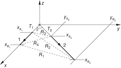
Figure C.13 Partial mutual inductance for two non-orthogonal filament wires in plane.
The integrals for two filaments are

where ![]() and
and ![]() are the two wire segments shown in Fig. C.13 and the dot product between the tangential vectors is
are the two wire segments shown in Fig. C.13 and the dot product between the tangential vectors is ![]() . This first result is derived from [1, 2]. The partial inductance between the filaments 1 and 2 is given by
. This first result is derived from [1, 2]. The partial inductance between the filaments 1 and 2 is given by

where

The following definitions are used for the two filaments:
The translations for the start of the wires are given by

were we use the notation for the angle ![]() :
:

where ![]() (like in equation C. 79).
(like in equation C. 79).
Again, this filament-to-filament partial mutual inductance is used in combination with numerical integration for different cross-sections, for example, [16].
This equation should be used if the wires are located in the same plane since this formula is simpler than the ones in the next sections. Please note that we did add a small number of the orientation of the wire such that parallel wires can be treated by this formula.
C.2.3  for Wire Filaments with an Arbitrary Direction
In this section, the filaments are oriented in any mutual orientation as shown in Fig. C.14. This allows an arbitrary relative orientation of the filaments. Using the rotation and translation operations in (C.2) to (C.5), we can place the two wires in any location in the global rectangular coordinate system. Hence, this result will be ideally suited for the filament representation of non-orthogonal quadrilateral and hexahedral shapes.
The integral for this case can be set up as

where the angle ![]() is defined as in [1] for the dot product and the vector is
is defined as in [1] for the dot product and the vector is
where ![]() and
and ![]() are the start and end point of filament 2, respectively, in the global coordinate system.
are the start and end point of filament 2, respectively, in the global coordinate system.
It is important to minimize the number of divisions and multiplications. For this reason, we present the formulation in a more compute friendly form

where

The following definitions are used for the arbitrary filaments:


The translations for the start of the wires are given by

Another definition from Grover we use is
were we use the notation for the angle ![]() :
:

Again, this filament-to-filament partial mutual inductance is used in combination with numerical integration for different cross-sections, for example, [16]. Please note that a small number could be added to the coordinates for parallel wires as we did in the formula for the in plane case in the previous section.
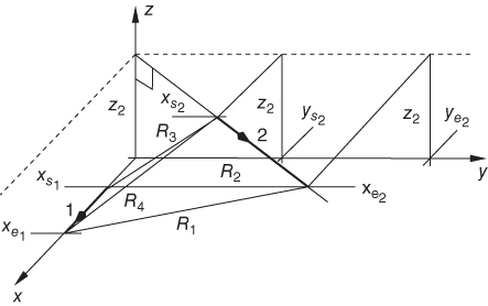
Figure C.14 Partial mutual inductance for two wires in arbitrary relative directions.
C.2.4  for Two Cells or Bars with Same Current Direction
In this example, we assume that all the current filaments are in the same direction, even if conductor cross sections are not parallel to the ![]() –
–![]() coordinates as shown in Figure C.15. In this case, the unit vectors are the same or,
coordinates as shown in Figure C.15. In this case, the unit vectors are the same or, ![]() . Hence, the wire-to-wire formula (C.8) or the sheet-to-wire inductance in Section C.1.3 can be utilized.
. Hence, the wire-to-wire formula (C.8) or the sheet-to-wire inductance in Section C.1.3 can be utilized.

Figure C.15 Arbitrary oriented rectangular bars.
Then, we can represent the partial inductance in the form

where ![]() . In this specific example, conductor 1 is in orthogonal coordinates and conductor 2 is in local coordinates.
. In this specific example, conductor 1 is in orthogonal coordinates and conductor 2 is in local coordinates.
Of course, if we apply the partial inductance for a sheet and a wire in (C.69), then the numerical integration for the sheet results in the numerical integration in the ![]() -direction for conductor 1 and in the
-direction for conductor 1 and in the ![]() and
and ![]() direction for conductor 2.
direction for conductor 2.
C.2.5  for Arbitrary Hexahedral Partial Self-Inductance
Progress in this area is also based on the Gauss law (3.33). Specifically, it was shown in Ref. [11] that the result is similar to quadrilateral surfaces (Section D.2.2). The resultant surface integral is obtained by starting with

With this, the integration over the surface of the hexahedral shape replaces the integration over the volume as in Refs. [12] and [13] similar to (7.34) for surfaces

where in this case, ![]() is the normal to the surface
is the normal to the surface ![]() . We should note that the dot product between the current directions for the partial self-terms is given by currents in the same direction.
. We should note that the dot product between the current directions for the partial self-terms is given by currents in the same direction.
The Gauss law was applied in the local coordinate domain in Ref. [14] and good results have been obtained using the Gauss law as well as other results using approximate shapes for some of the integrals yielded very good results in Ref. [13].
C.2.6  for Arbitrary Hexahedral Partial Mutual Inductance
The partial self- and mutual inductances for arbitrary hexahedral shapes are more challenging. We can use local coordinates to compute the partial mutual inductance for two arbitrarily placed hexahedral elements. An example for such elements is given in Refs [15, 16].
Figure C.16 shows two volume conductor cells. We assume that the local coordinate system for the first conductor is ![]() and
and ![]() for the second one. A vector in the global coordinates located on the first conductor is
for the second one. A vector in the global coordinates located on the first conductor is ![]() for the first hexahedral element, and another one is
for the first hexahedral element, and another one is ![]() . The current directions are indicated by dashed line are pointing in the
. The current directions are indicated by dashed line are pointing in the ![]() and
and ![]() directions as is shown in Fig. C.16 and
directions as is shown in Fig. C.16 and

where ![]() is the scalar Green's function
is the scalar Green's function


Figure C.16 General nonorthogonal hexahedral elements.
From the local coordinate system, we can determine a set of filaments in the global coordinate using the transform equations in section (8.2.6) to find the end points of each wire filament. Section D.2.2 can be used together with the numerical Gaussian integration. In Appendix E, the numerical integration is discussed which can be applied to the cross-sections to yield the partial inductance of interest.
To give more details, the local coordinate system presented in Chapter 8 is used to represent the hexahedral element shown in Fig. C.16. The purpose of the local coordinates is to identify the location of the points for the filaments in terms of the variables ![]() ,
, ![]() ,
, ![]() where
where ![]() and where
and where ![]() can represent
can represent ![]() . The purpose is to uniquely map a point
. The purpose is to uniquely map a point ![]() ,
, ![]() ,
, ![]() into a point in the global coordinates
into a point in the global coordinates ![]() . The local coordinates for the filament are used to map them to the global
. The local coordinates for the filament are used to map them to the global ![]() ,
, ![]() ,
, ![]() coordinates. Mapping a point in the above hexahedron from a local coordinate point
coordinates. Mapping a point in the above hexahedron from a local coordinate point ![]() ,
, ![]() ,
, ![]() to a global coordinate point
to a global coordinate point ![]() ,
, ![]() ,
, ![]() is described by
is described by

which is applied for ![]() . The coefficients in (C.86) are repeated here as
. The coefficients in (C.86) are repeated here as
where ![]() and again
and again ![]() . The close relation to the binary variables has been given before.
. The close relation to the binary variables has been given before.
With this, we are in a position to also express the tangential vectors with respect to the local coordinates as
where the derivatives are found from (C.86). Finally, the magnitude of the tangential vector ![]() where the position–dependent unit vectors can be determined from
where the position–dependent unit vectors can be determined from ![]() where again
where again ![]() .
.
With this transformation, we can simplify the sixfold integration into a two-area integration over the current directions ![]() and
and ![]() , respectively
, respectively

where ![]() and
and ![]() represent the two filaments. This is the partial mutual inductance between the two filaments pointing in
represent the two filaments. This is the partial mutual inductance between the two filaments pointing in ![]() and
and ![]() directions. Hence, for the volumes of the two conductors, the total partial mutual inductance between two hexahedrons is
directions. Hence, for the volumes of the two conductors, the total partial mutual inductance between two hexahedrons is

where the integration over the cross sections is performed with Gaussian numerical integration. This section is added to point out the difference between the local and global coordinates. Compute time can be saved if the numerical integration is mostly used for the smaller dimensions of the cell sides. Local coordinates are efficient for the mapping of the dimensions to the normalized units used for numerical integration methods.
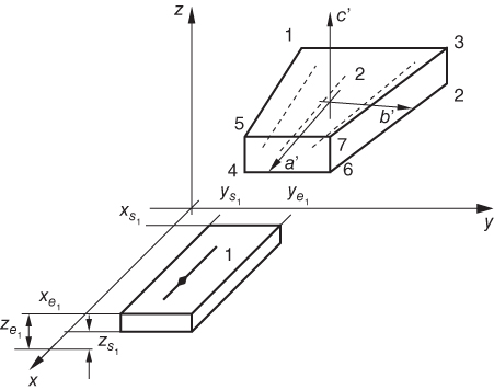
Figure C.17 Combined rectangular and quadrilateral cell example.
Local coordinates are only required for nonorthogonal conductor cell dimensions such as quadrilateral or hexahedral shapes. For the example in Fig. C.17, we can use mixed coordinates. Global coordinates are used for conductor cell 1 while local coordinates are used for conductor 2. The integrals are

Besides the change in the coordinate systems, the filament representation is the same as for the case in previous section. Representation is the same as for the case in the previous section. More details on nonorthogonal systems is given in Chapter 7.
References
- 1. F. W. Grover. Inductance Calculations: Working Formulas and Tables. Dover Publications, New York, 1962.
- 2. C. Paul. Inductance, Loop and Partial. John Wiley and Sons, Inc., New York, 2010.
- 3. C. Hoer and C. Love. Exact inductance equations for rectangular conductors with applications to more complicated geometries. Journal of Research National Bureau of Standards, Section C: Engineering and Instrumentation, 69(C):127–137, April 1965.
- 4. A. E. Ruehli. Inductance calculations in a complex integrated circuit environment. IBM Journal of Research and Development, 16(5):470–481, September 1972.
- 5. P. K. Wolff and A. E. Ruehli. Inductance computations for complex three dimensional geometries. In Proceedings of the IEEE International Symposium on Circuits and Systems, pp. 16–19, 1981.
- 6. A. Djordjevic and T. K. Sakkar. Computation of inductance of simple vias between two striplines above a ground plane. IEEE Transactions on Microwave Theory and Techniques, MTT-33(3):265–269, March 1985.
- 7. R.-B. Wu, C.-N. Kuo, and K. K. Chang. Inductance and resistance computations for three-dimensional multiconductor interconnection structures. IEEE Transactions on Microwave Theory and Techniques, MTT-40(2):263–270, February 1992.
- 8. A. E. Ruehli, G. Antonini, and L. Jiang. Skin-effect model for round wires in PEEC. In IEEE EMC Europe, Interantional Symposium on EMC, Rome, Italy, September 2012.
- 9. A. E. Ruehli, G. Antonini, and L. Jiang. Skin effect loss models for time and frequency domain PEEC solver. Proceedings of the IEEE, 101(2):451–472, February 2013.
- 10. G. Zhong and C.-K. Koh. Exact closed-form formula for partial mutual inductances rectangular conductors. IEEE Transactions on Circuits and Systems, 50(10):1349–1353, October 2003.
- 11. L. Knockaert. A general Gauss theorem for evaluating singular integrals over polyhedral domains. Electromagnetics, 11(2):269–280, April 1991.
- 12. R. Y. Zhang, J. K. White, and J. G. Kassakian. Fast simulation of complicated 3-D structures above lossy magnetic media. IEEE Transactions on Magnetics, 50(10):2377–3384, October 2014.
- 13. Y. Hackl, P. Scholz, W. Ackermann, and T. Weiland. Multifunction approach and specialized numerical integration algorithms for fast inductance evaluations in nonorthogonal PEEC systems. IEEE Transactions on Electromagnetic Compatibility, 57(5):1155–1163, October 2015.
- 14. M. A. Cracraft. Mobile array design with ANSERLIN antennas and efficient, wide-band PEEC models for interconnect and power distribution network analysis. Ph.D. Dissertation [Online]. Available: http://hdl.handle.net/10355/29582, Missouri University Science and Technology, USA, 2007.
- 15. A. Muesing and J. W. Kolar. Efficient partial element calculation and the extension to cylindrical elements for the PEEC method. in 2008 11th Workshop on Control and Modeling for Power Electronics, COMPEL, Zurich, August 2008.
- 16. A. Muesing, J. Ekman, and J. W. Kolar. Efficient calculation of non-orthogonal partial elements for the PEEC method. IEEE Transactions on Magnetics, 45(3):1140–1142, March 2009.