“Search” is such a broad term that this entire book could be called Classic Search Problems in Java. This chapter is about core search algorithms that every programmer should know. It does not claim to be comprehensive, despite the declaratory title.
2.1 DNA search
Genes are commonly represented in computer software as a sequence of the characters A, C, G, and T. Each letter represents a nucleotide, and the combination of three nucleotides is called a codon. This is illustrated in figure 2.1. A codon codes for a specific amino acid that together with other amino acids can form a protein. A classic task in bioinformatics software is to find a particular codon within a gene.
2.1.1 Storing DNA
We can represent a nucleotide as a simple enum with four cases.
package chapter2;

import java.util.ArrayList;
import java.util.Collections;
import java.util.Comparator;

public class Gene {

    public enum Nucleotide {
        A, C, G, T
    }

Figure 2.1 A nucleotide is represented by one of the letters A, C, G, and T. A codon is composed of three nucleotides, and a gene is composed of multiple codons.
Codons can be defined as a combination of three Nucleotides. The constructor for the Codon class converts a String of three letters into a Codon. To implement search methods, we will need to be able to compare one Codon to another. Java has an interface for that, Comparable.
Implementing the Comparable interface requires the construction of one method, compareTo(). compareTo() should return a negative number if the item in question is smaller than the item being compared, a zero if the two items are equal, and a positive number if the item is larger than the item being compared. In practice you can often avoid having to implement this by hand and instead use the built-in Java standard library interface Comparator, as we do in the following example. In this example, the Codon will first be compared to another Codon by its first Nucleotide, then by its second if the firsts are equivalent, and finally by its third if the seconds are equivalent. They are chained using thenComparing().
Listing 2.2 Gene.java continued
    public static class Codon implements Comparable<Codon> {
        public final Nucleotide first, second, third;
        private final Comparator<Codon> comparator = Comparator.comparing((Codon c) -> c.first)
                .thenComparing((Codon c) -> c.second)
                .thenComparing((Codon c) -> c.third);

        public Codon(String codonStr) {
            first = Nucleotide.valueOf(codonStr.substring(0, 1));
            second = Nucleotide.valueOf(codonStr.substring(1, 2));
            third = Nucleotide.valueOf(codonStr.substring(2, 3));
        }

        @Override
        public int compareTo(Codon other) {
            // first is compared first, then second, etc.
            // IOW first takes precedence over second
            // and second over third
            return comparator.compare(this, other);
        }
    }
Note Codon is a static class. Nested classes that are marked static can be instantiated without regard to their enclosing class (you do not need an instance of the enclosing class to create an instance of a static nested class), but they cannot refer to any of the instance variables of their enclosing class. This makes sense for classes that are defined as nested classes primarily for organizational purposes instead of logistical purposes.
Typically, genes on the internet will be in a file format that contains a giant string representing all of the nucleotides in the gene’s sequence. The next listing shows an example of what a gene string may look like.
Listing 2.3 Gene string example
String geneStr = "ACGTGGCTCTCTAACGTACGTACGTACGGGGTTTATATATACCCTAGGACTCCCTTT";
The only state in a Gene will be an ArrayList of Codons. We will also have a constructor that can take a gene string and convert it into a Gene (converting a String into an ArrayList of Codons).
Listing 2.4 Gene.java continued
private ArrayList<Codon> codons = new ArrayList<>();

public Gene(String geneStr) {
    for (int i = 0; i < geneStr.length() - 3; i += 3) {
        // Take every 3 characters in the String and form a Codon
        codons.add(new Codon(geneStr.substring(i, i + 3)));
    }
}
This constructor continually goes through the provided String and converts its next three characters into Codons that it adds to the end of a new Gene. It piggybacks on the constructor of Codon, which knows how to convert a three-letter String into a Codon.
2.1.2 Linear search
One basic operation we may want to perform on a gene is to search it for a particular codon. A scientist may want to do this to see if it codes for a particular amino acid. The goal is to simply find out whether the codon exists within the gene or not.
A linear search goes through every element in a search space, in the order of the original data structure, until what is sought is found or the end of the data structure is reached. In effect, a linear search is the most simple, natural, and obvious way to search for something. In the worst case, a linear search will require going through every element in a data structure, so it is of O(n) complexity, where n is the number of elements in the structure. This is illustrated in figure 2.2.

Figure 2.2 In the worst case of a linear search, you’ll sequentially look through every element of the array.
It is trivial to define a function that performs a linear search. It simply must go through every element in a data structure and check for its equivalence to the item being sought. You can use the following code in main() to test it.
Listing 2.5 Gene.java continued
    public boolean linearContains(Codon key) {
        for (Codon codon : codons) {
            if (codon.compareTo(key) == 0) {
                return true; // found a match
            }
        }
        return false;
    }

    public static void main(String[] args) {
        String geneStr = "ACGTGGCTCTCTAACGTACGTACGTACGGGGTTTATATATACCCTAGGACTCCCTTT";
        Gene myGene = new Gene(geneStr);
        Codon acg = new Codon("ACG");
        Codon gat = new Codon("GAT");
        System.out.println(myGene.linearContains(acg)); // true
        System.out.println(myGene.linearContains(gat)); // false
    }

}
Note This function is for illustrative purposes only. All of the classes in the Java standard library that implement the Collection interface (like ArrayList and LinkedList) have a contains() method that will likely be better optimized than anything we write.
2.1.3 Binary search
There is a faster way to search than looking at every element, but it requires us to know something about the order of the data structure ahead of time. If we know that the structure is sorted, and we can instantly access any item within it by its index, we can perform a binary search.
A binary search works by looking at the middle element in a sorted range of elements, comparing it to the element sought, reducing the range by half based on that comparison, and starting the process over again. Let’s look at a concrete example.
Suppose we have a list of alphabetically sorted words like ["cat", "dog", "kangaroo", "llama", "rabbit", "rat", "zebra"] and we are searching for the word “rat”:
-
We could determine that the middle element in this seven-word list is “llama.”
-
We could determine that “rat” comes after “llama” alphabetically, so it must be in the (approximately) half of the list that comes after “llama.” (If we had found “rat” in this step, we could have returned its location; if we had found that our word came before the middle word we were checking, we could be assured that it was in the half of the list before “llama.”)
-
We could rerun steps 1 and 2 for the half of the list that we know “rat” is still possibly in. In effect, this half becomes our new base list. These steps continually run until “rat” is found or the range we are looking in no longer contains any elements to search, meaning that “rat” does not exist within the word list.
Figure 2.3 illustrates a binary search. Notice that it does not involve searching every element, unlike a linear search.

Figure 2.3 In the worst case of a binary search, you’ll look through just lg(n) elements of the list.
A binary search continually reduces the search space by half, so it has a worst-case runtime of O(lg n). There is a sort-of catch, though. Unlike a linear search, a binary search requires a sorted data structure to search through, and sorting takes time. In fact, sorting takes O(n lg n) time for the best sorting algorithms. If we are only going to run our search once, and our original data structure is unsorted, it probably makes sense to just do a linear search. But if the search is going to be performed many times, the time cost of doing the sort is worth it, to reap the benefit of the greatly reduced time cost of each individual search.
Writing a binary search function for a gene and a codon is not unlike writing one for any other type of data, because the Codon type can be compared to others of its type, and the Gene type just contains an ArrayList of Codons. Note that in the following example we start by sorting the codons--this eliminates all of the advantages of doing a binary search, because doing the sort will take more time than the search, as described in the previous paragraph. However, for illustrative purposes, the sort is necessary, since we cannot know when running this example that the codons ArrayList is sorted.
Listing 2.6 Gene.java continued
public boolean binaryContains(Codon key) {
    // binary search only works on sorted collections
    ArrayList<Codon> sortedCodons = new ArrayList<>(codons);
    Collections.sort(sortedCodons);
    int low = 0;
    int high = sortedCodons.size() - 1;
    while (low <= high) { // while there is still a search space
        int middle = (low + high) / 2;
.get(middle).compareTo(key);
        if (comparison < 0) { // middle codon is less than key
            low = middle + 1;
        } else if (comparison > 0) { // middle codon is > key
            high = middle - 1;
        } else { // middle codon is equal to key
            return true;
        }
    }
    return false;
}
Let’s walk through this function line by line.
int low = 0;
int high = sortedCodons.size() - 1;
We start by looking at a range that encompasses the entire list (gene).
while (low <= high) {
We keep searching as long as there is still a range to search within. When low is greater than high, it means that there are no longer any slots to look at within the list.
int middle = (low + high) / 2;
We calculate the middle by using integer division and the simple mean formula you learned in grade school.
int comparison = codons.get(middle).compareTo(key);
if (comparison < 0) { // middle codon is less than key
    low = middle + 1;
If the element we are looking for is after the middle element of the range we are looking at, we modify the range that we will look at during the next iteration of the loop by moving low to be one past the current middle element. This is where we halve the range for the next iteration.
} else if (comparison > 0) { // middle codon is greater than key
    high = middle - 1;
Similarly, we halve in the other direction when the element we are looking for is less than the middle element.
} else { // middle codon is equal to key
    return true;
}
If the element in question is not less than or greater than the middle element, that means we found it! And, of course, if the loop ran out of iterations, we return false (not reproduced here), indicating that it was never found.
We can now try running our binary search method with the same gene and codon. We can modify main() to test it.
Listing 2.7 Gene.java continued
public static void main(String[] args) {
    String geneStr = "ACGTGGCTCTCTAACGTACGTACGTACGGGGTTTATATATACCCTAGGACTCCCTTT";
    Gene myGene = new Gene(geneStr);
    Codon acg = new Codon("ACG");
    Codon gat = new Codon("GAT");
    System.out.println(myGene.linearContains(acg)); // true
    System.out.println(myGene.linearContains(gat)); // false
    System.out.println(myGene.binaryContains(acg)); // true
    System.out.println(myGene.binaryContains(gat)); // false
}
TIP Once again, like with linear search, you would never need to implement binary search yourself because there’s an implementation in the Java standard library. Collections.binarySearch() can search any sorted Collection (like a sorted ArrayList).
2.1.4 A generic example
The methods linearContains() and binaryContains() can be generalized to work with almost any Java List. The following generalized versions are nearly identical to the versions you saw before, with only some names and types changed.
Note There are many imported types in the following code listing. We will be reusing the file GenericSearch.java for many further generic search algorithms in this chapter, and this gets the imports out of the way.
Note The extends keyword in T extends Comparable<T> means that T must be a type that implements the Comparable interface.
Listing 2.8 GenericSearch.java
package chapter2;

import java.util.ArrayList;
import java.util.HashMap;
import java.util.HashSet;
import java.util.LinkedList;
import java.util.List;
import java.util.Map;
import java.util.PriorityQueue;
import java.util.Queue;
import java.util.Set;
import java.util.Stack;
import java.util.function.Function;
import java.util.function.Predicate;
import java.util.function.ToDoubleFunction;

public class GenericSearch {

    public static <T extends Comparable<T>> boolean linearContains(List<T> list, T key) {
        for (T item : list) {
            if (item.compareTo(key) == 0) {
                return true; // found a match
            }
        }
        return false;
    }

    // assumes *list* is already sorted
    public static <T extends Comparable<T>> boolean binaryContains(List<T> list, T key) {
        int low = 0;
        int high = list.size() - 1;
        while (low <= high) { // while there is still a search space
            int middle = (low + high) / 2;
            int comparison = list.get(middle).compareTo(key);
            if (comparison < 0) { // middle codon is < key
                low = middle + 1;
            } else if (comparison > 0) { // middle codon is > key
                high = middle - 1;
            } else { // middle codon is equal to key
                return true;
            }
        }
        return false;
    }

    public static void main(String[] args) {
        System.out.println(linearContains(List.of(1, 5, 15, 15, 15, 15, 20), 5)); // true
        System.out.println(binaryContains(List.of("a", "d", "e", "f", "z"), "f")); // true
        System.out.println(binaryContains(List.of("john", "mark", "ronald", "sarah"), "sheila")); // false
    }

}
Now you can try doing searches on other types of data. These methods will work on any List of Comparables. That is the power of writing code generically.
2.2 Maze solving
Finding a path through a maze is analogous to many common search problems in computer science. Why not literally find a path through a maze, then, to illustrate the breadth-first search, depth-first search, and A* algorithms?
Our maze will be a two-dimensional grid of Cells. A Cell is an enum that knows how to turn itself into a String. For example, " " will represent an empty space, and "X" will represent a blocked space. There are also other cases for illustrative purposes when printing a maze.
package chapter2;

import java.util.ArrayList;
import java.util.Arrays;
import java.util.List;

import chapter2.GenericSearch.Node;

public class Maze {

    public enum Cell {
        EMPTY(" "),
        BLOCKED("X"),
        START("S"),
        GOAL("G"),
        PATH("*");

        private final String code;

        private Cell(String c) {
            code = c;
        }

        @Override
        public String toString() {
            return code;
        }
    }
Once again, we are getting a few imports out of the way. Note that the last import (from GenericSearch) is of a class we have not yet defined. It is included here for convenience, but you may want to comment it out until you need it.
We will need a way to refer to an individual location in the maze. This will be a simple class, MazeLocation, with properties representing the row and column of the location in question. However, the class will also need a way for instances of it to compare themselves for equality to other instances of the same type. In Java, this is necessary to properly use several classes in the collections framework, like HashSet and HashMap. They use the methods equals() and hashCode() to avoid inserting duplicates, since they only allow unique instances.
Luckily, IDEs can do the hard work for us. The two methods following the constructor in the next listing were autogenerated by Eclipse. They will ensure two instances of MazeLocation with the same row and column are seen as equivalent to one another. In Eclipse, you can right-click and select Source > Generate hashCode() and equals() to have these methods created for you. You need to specify in a dialog which instance variables go into evaluating equality.
Listing 2.10 Maze.java continued
public static class MazeLocation {
    public final int row;
    public final int column;

    public MazeLocation(int row, int column) {
        this.row = row;
        this.column = column;
    }

    // auto-generated by Eclipse
    @Override
    public int hashCode() {
        final int prime = 31;
        int result = 1;
        result = prime * result + column;
        result = prime * result + row;
        return result;
    }

    // auto-generated by Eclipse
    @Override
    public boolean equals(Object obj) {
        if (this == obj) {
            return true;
        }
        if (obj == null) {
            return false;
        }
        if (getClass() != obj.getClass()) {
            return false;
        }
        MazeLocation other = (MazeLocation) obj;
        if (column != other.column) {
            return false;
        }
        if (row != other.row) {
            return false;
        }
        return true;
    }
}
2.2.1 Generating a random maze
Our Maze class will internally keep track of a grid (a two-dimensional array) representing its state. It will also have instance variables for the number of rows, number of columns, start location, and goal location. Its grid will be randomly filled with blocked cells.
The maze that is generated should be fairly sparse so that there is almost always a path from a given starting location to a given goal location. (This is for testing our algorithms, after all.) We’ll let the caller of a new maze decide on the exact sparseness, but we will provide a default value of 20% blocked. When a random number beats the threshold of the sparseness parameter in question, we will simply replace an empty space with a wall. If we do this for every possible place in the maze, statistically, the sparseness of the maze as a whole will approximate the sparseness parameter supplied.
Listing 2.11 Maze.java continued
private final int rows, columns;
private final MazeLocation start, goal;
private Cell[][] grid;

public Maze(int rows, int columns, MazeLocation start, MazeLocation goal, double sparseness) {
    // initialize basic instance variables
    this.rows = rows;
    this.columns = columns;
    this.start = start;
    this.goal = goal;
    // fill the grid with empty cells
    grid = new Cell[rows][columns];
    for (Cell[] row : grid) {
        Arrays.fill(row, Cell.EMPTY);
    }
    // populate the grid with blocked cells
    randomlyFill(sparseness);
    // fill the start and goal locations
    grid[start.row][start.column] = Cell.START;
    grid[goal.row][goal.column] = Cell.GOAL;
}

public Maze() {
    this(10, 10, new MazeLocation(0, 0), new MazeLocation(9, 9), 0.2);
}
private void randomlyFill(double sparseness) {
    for (int row = 0; row < rows; row++) {
        for (int column = 0; column < columns; column++) {
            if (Math.random() < sparseness) {
                grid[row][column] = Cell.BLOCKED;
            }
        }
    }
}
Now that we have a maze, we also want a way to print it succinctly to the console. We want its characters to be close together so it looks like a real maze.
Listing 2.12 Maze.java continued
// return a nicely formatted version of the maze for printing
@Override
public String toString() {
    StringBuilder sb = new StringBuilder();
    for (Cell[] row : grid) {
        for (Cell cell : row) {
            sb.append(cell.toString());
        }
        sb.append(System.lineSeparator());
    }
    return sb.toString();
}
Go ahead and test these maze functions in main() if you like.
Listing 2.13 Maze.java continued
    public static void main(String[] args) {
        Maze m = new Maze();
        System.out.println(m);
    }

}
2.2.2 Miscellaneous maze minutiae
It will be handy later to have a function that checks whether we have reached our goal during the search. In other words, we want to check whether a particular MazeLocation that the search has reached is the goal. We can add a method to Maze.
Listing 2.14 Maze.java continued
public boolean goalTest(MazeLocation ml) {
    return goal.equals(ml);
}
How can we move within our mazes? Let’s say that we can move horizontally and vertically one space at a time from a given space in the maze. Using these criteria, a successors() function can find the possible next locations from a given MazeLocation. However, the successors() function will differ for every Maze because every Maze has a different size and set of walls. Therefore, we will define it as a method on Maze.
Listing 2.15 Maze.java continued
public List<MazeLocation> successors(MazeLocation ml) {
    List<MazeLocation> locations = new ArrayList<>();
    if (ml.row + 1 < rows && grid[ml.row + 1][ml.column] != Cell.BLOCKED) {
        locations.add(new MazeLocation(ml.row + 1, ml.column));
    }
    if (ml.row - 1 >= 0 && grid[ml.row - 1][ml.column] != Cell.BLOCKED) {
        locations.add(new MazeLocation(ml.row - 1, ml.column));
    }
    if (ml.column + 1 < columns && grid[ml.row][ml.column + 1] != Cell.BLOCKED) {
        locations.add(new MazeLocation(ml.row, ml.column + 1));
    }
    if (ml.column - 1 >= 0 && grid[ml.row][ml.column - 1] != Cell.BLOCKED) {
        locations.add(new MazeLocation(ml.row, ml.column - 1));
    }
    return locations;
}
successors() simply checks above, below, to the right, and to the left of a MazeLocation in a Maze to see if it can find empty spaces that can be gone to from that location. It also avoids checking locations beyond the edges of the Maze. It puts every possible MazeLocation that it finds into a list that it ultimately returns to the caller. We will use the prior two methods in our search algorithms.
2.2.3 Depth-first search
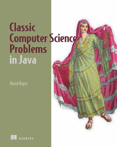
A depth-first search (DFS) is what its name suggests: a search that goes as deeply as it can before backtracking to its last decision point if it reaches a dead end. We’ll implement a generic depth-first search that can solve our maze problem. It will also be reusable for other problems. Figure 2.4 illustrates an in-progress depth-first search of a maze.
The depth-first search algorithm relies on a data structure known as a stack. (We first saw stacks in chapter 1.) A stack is a data structure that operates under the Last-In-First-Out (LIFO) principle. Imagine a stack of papers. The last paper placed on top of the stack is the first paper pulled off the stack. It is common for a stack to be implemented on top of a more primitive data structure like a linked list by adding items on one end and removing them from the same end. We could easily implement a stack ourselves, but the Java standard library includes the convenient Stack class.
Stacks generally have at least two operations:
Figure 2.4 In depth-first search, the search proceeds along a continuously deeper path until it hits a barrier and must backtrack to the last decision point.
In other words, a stack is a meta-structure that enforces an ordering of removal on a list. The last item put into a stack must be the next item removed from a stack.
We will need one more little tidbit before we can get to implementing DFS. We need a Node class that we will use to keep track of how we got from one state to another state (or from one place to another place) as we search. You can think of a Node as a wrapper around a state. In the case of our maze-solving problem, those states are of type MazeLocation. We’ll call the Node that a state came from its parent. We will also define our Node class as having cost and heuristic properties, so we can reuse it later in the A* algorithm. Don’t worry about them for now. A Node is Comparable by comparing the combination of its cost and heuristic.
Listing 2.16 GenericSearch.java continued
public static class Node<T> implements Comparable<Node<T>> {
    final T state;
    Node<T> parent;
    double cost;
    double heuristic;
    // for dfs and bfs we won't use cost and heuristic
    Node(T state, Node<T> parent) {
        this.state = state;
        this.parent = parent;
    }

    // for astar we will use cost and heuristic
    Node(T state, Node<T> parent, double cost, double heuristic) {
        this.state = state;
        this.parent = parent;
        this.cost = cost;
        this.heuristic = heuristic;
    }

    @Override
    public int compareTo(Node<T> other) {
        Double mine = cost + heuristic;
        Double theirs = other.cost + other.heuristic;
        return mine.compareTo(theirs);
    }
}
TIP compareTo() here works by calling compareTo() on another type. This is a common pattern.
NoTe If a Node does not have a parent, we will use null as a sentinel to indicate such.
An in-progress depth-first search needs to keep track of two data structures: the stack of states (or “places”) that we are considering searching, which we will call the frontier, and the set of states that we have already searched, which we will call explored. As long as there are more states to visit in the frontier, DFS will keep checking whether they are the goal (if a state is the goal, DFS will stop and return it) and adding their successors to the frontier. It will also mark each state that has already been searched as explored, so that the search does not get caught in a circle, reaching states that have prior visited states as successors. If the frontier is empty, it means there is nowhere left to search.
Listing 2.17 GenericSearch.java continued
public static <T> Node<T> dfs(T initial, Predicate<T> goalTest,
        Function<T, List<T>> successors) {
    // frontier is where we've yet to go
    Stack<Node<T>> frontier = new Stack<>();
    frontier.push(new Node<>(initial, null));
    // explored is where we've been
    Set<T> explored = new HashSet<>();
    explored.add(initial);

    // keep going while there is more to explore
    while (!frontier.isEmpty()) {
        Node<T> currentNode = frontier.pop();
        T currentState = currentNode.state;
        // if we found the goal, we're done
        if (goalTest.test(currentState)) {
            return currentNode;
        }
        // check where we can go next and haven't explored
        for (T child : successors.apply(currentState)) {
            if (explored.contains(child)) {
                continue; // skip children we already explored
            }
            explored.add(child);
            frontier.push(new Node<>(child, currentNode));
        }
    }
    return null; // went through everything and never found goal
}
Note the goalTest and successors function references. These allow different functions to be plugged into dfs() for different applications. This makes dfs() usable by more scenarios than just mazes. This is another example of solving a problem generically. A goalTest, being a Predicate<T>, is any function that takes a T (in our case, a MazeLocation) and returns a boolean. successors is any function that takes a T and returns a List of T.
If dfs() is successful, it returns the Node encapsulating the goal state. The path from the start to the goal can be reconstructed by working backward from this Node and its priors using the parent property.
Listing 2.18 GenericSearch.java continued
public static <T> List<T> nodeToPath(Node<T> node) {
    List<T> path = new ArrayList<>();
    path.add(node.state);
    // work backwards from end to front
    while (node.parent != null) {
        node = node.parent;
        path.add(0, node.state); // add to front
    }
    return path;
}
For display purposes, it will be useful to mark up the maze with the successful path, the start state, and the goal state. It will also be useful to be able to remove a path so that we can try different search algorithms on the same maze. The following two methods should be added to the Maze class in Maze.java.
Listing 2.19 Maze.java continued
public void mark(List<MazeLocation> path) {
    for (MazeLocation ml : path) {
        grid[ml.row][ml.column] = Cell.PATH;
    }
    grid[start.row][start.column] = Cell.START;
    grid[goal.row][goal.column] = Cell.GOAL;
}

public void clear(List<MazeLocation> path) {
    for (MazeLocation ml : path) {
        grid[ml.row][ml.column] = Cell.EMPTY;
    }
    grid[start.row][start.column] = Cell.START;
    grid[goal.row][goal.column] = Cell.GOAL;
}
It has been a long journey, but we are finally ready to solve the maze.
Listing 2.20 Maze.java continued
public static void main(String[] args) {
    Maze m = new Maze();
    System.out.println(m);

    Node<MazeLocation> solution1 = GenericSearch.dfs(m.start, m::goalTest, m::successors);
    if (solution1 == null) {
        System.out.println("No solution found using depth-first search!");
    } else {
        List<MazeLocation> path1 = GenericSearch.nodeToPath(solution1);
        m.mark(path1);
        System.out.println(m);
        m.clear(path1);
    }
}
}
A successful solution will look something like this:
S****X X
 X  *****
       X*
 XX******X
  X*
  X**X
 X  *****
        *
     X  *X
        *G
The asterisks represent the path that our depth-first search function found from the start to the goal. S is the start location and G is the goal location. Remember, because each maze is randomly generated, not every maze has a solution.
2.2.4 Breadth-first search
You may notice that the solution paths to the mazes found by depth-first traversal seem unnatural. They are usually not the shortest paths. Breadth-first search (BFS) always finds the shortest path by systematically looking one layer of nodes farther away from the start state in each iteration of the search. There are particular problems in which a depth-first search is likely to find a solution more quickly than a breadth-first search, and vice versa. Therefore, choosing between the two is sometimes a trade-off between the possibility of finding a solution quickly and the certainty of finding the shortest path to the goal (if one exists). Figure 2.5 illustrates an in-progress breadth-first search of a maze.

Figure 2.5 In a breadth-first search, the closest elements to the starting location are searched first.
To understand why a depth-first search sometimes returns a result faster than a breadth-first search, imagine looking for a marking on a particular layer of an onion. A searcher using a depth-first strategy may plunge a knife into the center of the onion and haphazardly examine the chunks cut out. If the marked layer happens to be near the chunk cut out, there is a chance that the searcher will find it more quickly than another searcher using a breadth-first strategy, who painstakingly peels the onion one layer at a time.
To get a better picture of why breadth-first search always finds the shortest solution path where one exists, consider trying to find the path with the fewest number of stops between Boston and New York by train. If you keep going in the same direction and backtracking when you hit a dead end (as in depth-first search), you may first find a route all the way to Seattle before it connects back to New York. However, in a breadth-first search, you will first check all of the stations one stop away from Boston. Then you will check all of the stations two stops away from Boston. Then you will check all of the stations three stops away from Boston. This will keep going until you find New York. Therefore, when you do find New York, you will know you have found the route with the fewest stops, because you already checked all of the stations that are fewer stops away from Boston, and none of them was New York.
To implement BFS, a data structure known as a queue is required. Whereas a stack is LIFO, a queue is FIFO (First-In-First-Out). A queue is like a line to use a restroom. The first person who got in line goes to the restroom first. At a minimum, a queue has the same push() and pop() methods as a stack. At an implementation level, the only thing that changes between a stack and a queue is that the queue removes items from the list at the opposite end from where it inserts them. This ensures that the oldest elements (the elements “waiting” the longest) are always removed first.
NOTE Confusingly, the Java standard library does not have a Queue class, although it does have a Stack class. Instead it has a Queue interface that several Java standard library classes implement (including LinkedList). Even more confusingly, in the Java standard library’s Queue interface, push() is called offer() and pop() is called poll().
Amazingly, the algorithm for a breadth-first search is identical to the algorithm for a depth-first search, with the frontier changed from a stack to a queue. Changing the frontier from a stack to a queue changes the order in which states are searched and ensures that the states closest to the start state are searched first.
In the following implementation, we also have to change some calls from push() and pop() to offer() and poll(), respectively, because of the different naming schemes between the Java standard library’s Stack class and Queue interface (see the previous note). But do take a moment to look back at dfs() (in listing 2.17) and admire how similar dfs() and bfs() are to one another, with just the frontier data structure changing.
Listing 2.21 GenericSearch.java continued
public static <T> Node<T> bfs(T initial, Predicate<T> goalTest,
        Function<T, List<T>> successors) {
    // frontier is where we've yet to go
    Queue<Node<T>> frontier = new LinkedList<>();
    frontier.offer(new Node<>(initial, null));
    // explored is where we've been
    Set<T> explored = new HashSet<>();
    explored.add(initial);

    // keep going while there is more to explore
    while (!frontier.isEmpty()) {
        Node<T> currentNode = frontier.poll();
        T currentState = currentNode.state;
        // if we found the goal, we're done
        if (goalTest.test(currentState)) {
            return currentNode;
        }
        // check where we can go next and haven't explored
        for (T child : successors.apply(currentState)) {
            if (explored.contains(child)) {
                continue; // skip children we already explored
            }
            explored.add(child);
            frontier.offer(new Node<>(child, currentNode));
        }
    }
    return null; // went through everything and never found goal
}
If you try running bfs(), you will see that it always finds the shortest solution to the maze in question. The main() method in Maze.java can now be modified to try two different ways of solving the same maze, so results can be compared.
Listing 2.22 Maze.java continued
public static void main(String[] args) {
    Maze m = new Maze();
    System.out.println(m);

    Node<MazeLocation> solution1 = GenericSearch.dfs(m.start, m::goalTest, m::successors);
    if (solution1 == null) {
        System.out.println("No solution found using depth-first search!");
    } else {
        List<MazeLocation> path1 = GenericSearch.nodeToPath(solution1);
        m.mark(path1);
        System.out.println(m);
        m.clear(path1);
    }

    Node<MazeLocation> solution2 = GenericSearch.bfs(m.start, m::goalTest, m::successors);
    if (solution2 == null) {
        System.out.println("No solution found using breadth-first search!");
    } else {
        List<MazeLocation> path2 = GenericSearch.nodeToPath(solution2);
        m.mark(path2);
        System.out.println(m);
        m.clear(path2);
    }
}
It is amazing that you can keep an algorithm the same and just change the data structure that it accesses and get radically different results. The following is the result of calling bfs() on the same maze that we earlier called dfs() on. Notice how the path marked by the asterisks is more direct from start to goal than in the prior example.
S    X X
*X
*      X
*XX      X
* X
* X  X
*X
*
*    X   X
*********G
2.2.5 A* search
It can be very time-consuming to peel back an onion, layer by layer, as a breadth-first search does. Like a BFS, an A* search aims to find the shortest path from start state to goal state. But unlike the preceding BFS implementation, an A* search uses a combination of a cost function and a heuristic function to focus its search on pathways most likely to get to the goal quickly.
The cost function, g(n), examines the cost to get to a particular state. In the case of our maze, this would be how many previous cells we had to go through to get to the cell in question. The heuristic function, h(n), gives an estimate of the cost to get from the state in question to the goal state. It can be proved that if h(n) is an admissible heuristic, the final path found will be optimal. An admissible heuristic is one that never overestimates the cost to reach the goal. On a two-dimensional plane, one example is a straight-line distance heuristic, because a straight line is always the shortest path.1
The total cost for any state being considered is f(n), which is simply the combination of g(n) and h(n). In fact, f(n) = g(n) + h(n). When choosing the next state to explore from the frontier, an A* search picks the one with the lowest f(n). This is how it distinguishes itself from BFS and DFS.
To pick the state on the frontier with the lowest f(n), an A* search uses a priority queue as the data structure for its frontier. A priority queue keeps its elements in an internal order, such that the first element popped out is always the highest-priority element. (In our case, the highest-priority item is the one with the lowest f(n).) Usually this means the internal use of a binary heap, which results in O(lg n) pushes and O(lg n) pops.
Java’s standard library contains the PriorityQueue class, which has the same offer() and poll() methods as the Queue interface. Anything put into a PriorityQueue must be Comparable. To determine the priority of a particular element versus another of its kind, PriorityQueue compares them by using the compareTo() method. This is why we needed to implement it earlier. One Node is compared to another by looking at its respective f(n), which is simply the sum of the properties cost and heuristic.
A heuristic is an intuition about the way to solve a problem.2 In the case of maze solving, a heuristic aims to choose the best maze location to search next in the quest to get to the goal. In other words, it is an educated guess about which nodes on the frontier are closest to the goal. As was mentioned previously, if a heuristic used with an A* search produces an accurate relative result and is admissible (never overestimates the distance), then A* will deliver the shortest path. Heuristics that calculate smaller values end up leading to a search through more states, whereas heuristics closer to the exact real distance (but not over it, which would make them inadmissible) lead to a search through fewer states. Therefore, ideal heuristics come as close to the real distance as possible without ever going over it.
As we learn in geometry, the shortest path between two points is a straight line. It makes sense, then, that a straight-line heuristic will always be admissible for the maze-solving problem. The Euclidean distance, derived from the Pythagorean theorem, states that distance = √((difference in x)2 + (difference in y)2). For our mazes, the difference in x is equivalent to the difference in columns between two maze locations, and the difference in y is equivalent to the difference in rows. Note that we are implementing this back in Maze.java.
Listing 2.23 Maze.java continued
public double euclideanDistance(MazeLocation ml) {
    int xdist = ml.column - goal.column;
    int ydist = ml.row - goal.row;
    return Math.sqrt((xdist * xdist) + (ydist * ydist));
}
euclideanDistance() is a function that takes a maze location and returns its straight-line distance to the goal. This function “knows” the goal, because it is actually a method on Maze, and Maze has goal as an instance variable.
Figure 2.6 illustrates Euclidean distance within the context of a grid, like the streets of Manhattan.

Figure 2.6 Euclidean distance is the length of a straight line from the starting point to the goal.
Euclidean distance is great, but for our particular problem (a maze in which you can move only in one of four directions) we can do even better. The Manhattan distance is derived from navigating the streets of Manhattan, the most famous of New York City’s boroughs, which is laid out in a grid pattern. To get from anywhere to anywhere in Manhattan, one needs to walk a certain number of horizontal blocks and a certain number of vertical blocks. (There are almost no diagonal streets in Manhattan.) The Manhattan distance is derived by simply finding the difference in rows between two maze locations and summing it with the difference in columns. Figure 2.7 illustrates Manhattan distance.
Listing 2.24 Maze.java continued
public double manhattanDistance(MazeLocation ml) {
    int xdist = Math.abs(ml.column - goal.column);
    int ydist = Math.abs(ml.row - goal.row);
    return (xdist + ydist);
}
Because this heuristic more accurately follows the actuality of navigating our mazes (moving vertically and horizontally instead of in diagonal straight lines), it comes closer to the actual distance between any maze location and the goal than Euclidean distance does. Therefore, when an A* search is coupled with Manhattan distance, it will result in searching through fewer states than when an A* search is coupled with Euclidean distance for our mazes. Solution paths will still be optimal, because Manhattan distance is admissible (never overestimates distance) for mazes in which only four directions of movement are allowed.

Figure 2.7 In Manhattan distance, there are no diagonals. The path must be along parallel or perpendicular lines.
To go from BFS to A* search, we need to make several small modifications. The first is changing the frontier from a queue to a priority queue. This way, the frontier will pop nodes with the lowest f(n). The second is changing the explored set to a HashMap. A HashMap will allow us to keep track of the lowest cost (g(n)) of each node we may visit. With the heuristic function now in play, it is possible some nodes may be visited twice if the heuristic is inconsistent. If the node found through the new direction has a lower cost to get to than the prior time we visited it, we will prefer the new route.
For the sake of simplicity, the method astar() does not take a cost-calculation function as a parameter. Instead, we just consider every hop in our maze to be a cost of 1. Each new Node gets assigned a cost based on this simple formula, as well as a heuristic score using a new function passed as a parameter to the search function, called heuristic. Other than these changes, astar() is remarkably similar to bfs(). Examine them side by side for comparison.
Listing 2.25 GenericSearch.java continued
public static <T> Node<T> astar(T initial, Predicate<T> goalTest,
        Function<T, List<T>> successors, ToDoubleFunction<T> heuristic) {
    // frontier is where we've yet to go
    PriorityQueue<Node<T>> frontier = new PriorityQueue<>();
    frontier.offer(new Node<>(initial, null, 0.0, heuristic.applyAsDouble(initial)));
    // explored is where we've been
    Map<T, Double> explored = new HashMap<>();
    explored.put(initial, 0.0);
    // keep going while there is more to explore
    while (!frontier.isEmpty()) {
        Node<T> currentNode = frontier.poll();
        T currentState = currentNode.state;
        // if we found the goal, we're done
        if (goalTest.test(currentState)) {
            return currentNode;
        }
        // check where we can go next and haven't explored
        for (T child : successors.apply(currentState)) {
            // 1 here assumes a grid, need a cost function for more sophisticated apps
            double newCost = currentNode.cost + 1;
            if (!explored.containsKey(child) || explored.get(child) > newCost) {
                explored.put(child, newCost);
                frontier.offer(new Node<>(child, currentNode, newCost, heuristic.applyAsDouble(child)));
            }
        }
    }

    return null; // went through everything and never found goal
}
Congratulations. If you have followed along this far, you have learned not only how to solve a maze, but also some generic search functions that you can use in many different search applications. DFS and BFS are suitable for many smaller data sets and state spaces where performance is not critical. In some situations, DFS will outperform BFS, but BFS has the advantage of always delivering an optimal path. Interestingly, BFS and DFS have identical implementations, only differentiated by the use of a queue instead of a stack for the frontier. The slightly more complicated A* search, coupled with a good, consistent, admissible heuristic, not only delivers optimal paths, but also far outperforms BFS. And because all three of these functions were implemented generically, using them on nearly any search space is just an import away.
Go ahead and try out astar() with the same maze in Maze.java’s testing section.
Listing 2.26 Maze.java continued
public static void main(String[] args) {
    Maze m = new Maze();
    System.out.println(m);

    Node<MazeLocation> solution1 = GenericSearch.dfs(m.start, m::goalTest, m::successors);
    if (solution1 == null) {
        System.out.println("No solution found using depth-first search!");
    } else {
        List<MazeLocation> path1 = GenericSearch.nodeToPath(solution1);
        m.mark(path1);
        System.out.println(m);
        m.clear(path1);
    }
    Node<MazeLocation> solution2 = GenericSearch.bfs(m.start, m::goalTest, m::successors);
    if (solution2 == null) {
        System.out.println("No solution found using breadth-first search!");
    } else {
        List<MazeLocation> path2 = GenericSearch.nodeToPath(solution2);
        m.mark(path2);
        System.out.println(m);
        m.clear(path2);
    }

    Node<MazeLocation> solution3 = GenericSearch.astar(m.start, m::goalTest, m::successors, m::manhattanDistance);
    if (solution3 == null) {
        System.out.println("No solution found using A*!");
    } else {
        List<MazeLocation> path3 = GenericSearch.nodeToPath(solution3);
        m.mark(path3);
        System.out.println(m);
        m.clear(path3);
    }
}
The output will interestingly be a little different from bfs(), even though both bfs() and astar() are finding optimal paths (equivalent in length). If it uses a Manhattan distance heuristic, astar() immediately drives through a diagonal toward the goal. It will ultimately search fewer states than bfs(), resulting in better performance. Add a state count to each if you want to prove this to yourself.
S**  X X
 X**
   *   X
 XX*     X
  X*
  X**X
 X  ****
       *
     X * X
       **G
2.3 Missionaries and cannibals
Three missionaries and three cannibals are on the west bank of a river. They have a canoe that can hold two people, and they all must cross to the east bank of the river. There may never be more cannibals than missionaries on either side of the river, or the cannibals will eat the missionaries. Further, the canoe must have at least one person on board to cross the river. What sequence of crossings will successfully take the entire party across the river? Figure 2.8 illustrates the problem.
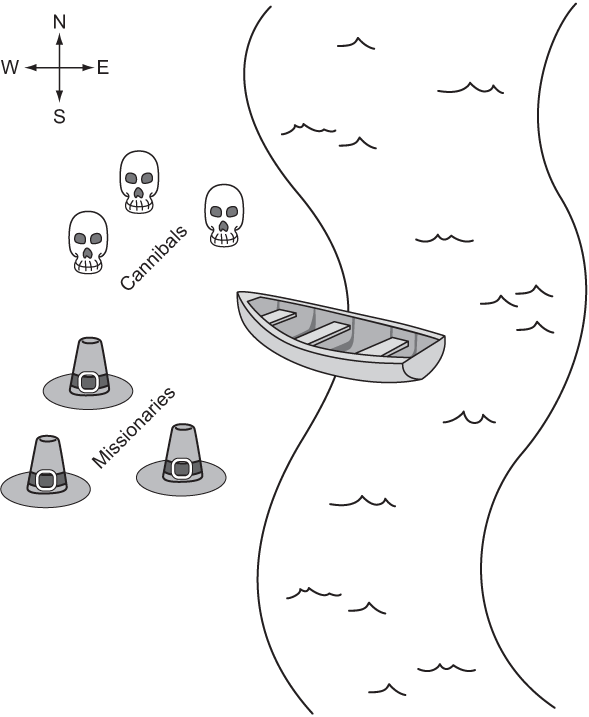
Figure 2.8 The missionaries and cannibals must use their single canoe to take everyone across the river from west to east. If the cannibals ever outnumber the missionaries, they will eat them.
2.3.1 Representing the problem
We will represent the problem by having a structure that keeps track of the west bank. How many missionaries and cannibals are on the west bank? Is the boat on the west bank? Once we have this knowledge, we can figure out what is on the east bank, because anything not on the west bank is on the east bank.
First, we will create a little convenience variable for keeping track of the maximum number of missionaries or cannibals. Then we will define the main class.
Listing 2.27 Missionaries.java
package chapter2;

import java.util.ArrayList;
import java.util.List;
import java.util.function.Predicate;

import chapter2.GenericSearch.Node;

public class MCState {
    private static final int MAX_NUM = 3;
    private final int wm; // west bank missionaries
    private final int wc; // west bank cannibals
    private final int em; // east bank missionaries
    private final int ec; // east bank cannibals
    private final boolean boat; // is boat on west bank?
    public MCState(int missionaries, int cannibals, boolean boat) {
        wm = missionaries;
        wc = cannibals;
        em = MAX_NUM - wm;
        ec = MAX_NUM - wc;
        this.boat = boat;
    }

    @Override
    public String toString() {
        return String.format(
        "On the west bank there are %d missionaries and %d cannibals.%n"
        + "On the east bank there are %d missionaries and %d cannibals.%n"
        + "The boat is on the %s bank.","
        wm, wc, em, ec,
        boat ? "west" : "east");
    }
The class MCState initializes itself based on the number of missionaries and cannibals on the west bank as well as the location of the boat. It also knows how to pretty-print itself, which will be valuable later when displaying the solution to the problem.
Working within the confines of our existing search functions means that we must define a function for testing whether a state is the goal state and a function for finding the successors from any state. The goal test function, as in the maze-solving problem, is quite simple. The goal is simply reaching a legal state that has all of the missionaries and cannibals on the east bank. We add it as a method to MCState.
Listing 2.28 Missionaries.java continued
public boolean goalTest() {
    return isLegal() && em == MAX_NUM && ec == MAX_NUM;
}
To create a successors function, it is necessary to go through all of the possible moves that can be made from one bank to another and then check if each of those moves will result in a legal state. Recall that a legal state is one in which cannibals do not outnumber missionaries on either bank. To determine this, we can define a convenience method on MCState that checks if a state is legal.
Listing 2.29 Missionaries.java continued
public boolean isLegal() {
    if (wm < wc && wm > 0) {
        return false;
    }
    if (em < ec && em > 0) {
        return false;
    }
    return true;
}
The actual successors function is a bit verbose, for the sake of clarity. It tries adding every possible combination of one or two people moving across the river from the bank where the canoe currently resides. Once it has added all possible moves, it filters for the ones that are actually legal via removeIf() on a temporary List of potential states and a negated Predicate that checks isLegal(). Predicate.not() was added in Java 11. Once again, this is a method on MCState.
Listing 2.30 Missionaries.java continued
public static List<MCState> successors(MCState mcs) {
    List<MCState> sucs = new ArrayList<>();
    if (mcs.boat) { // boat on west bank
        if (mcs.wm > 1) {
            sucs.add(new MCState(mcs.wm - 2, mcs.wc, !mcs.boat));
        }
        if (mcs.wm > 0) {
            sucs.add(new MCState(mcs.wm - 1, mcs.wc, !mcs.boat));
        }
        if (mcs.wc > 1) {
            sucs.add(new MCState(mcs.wm, mcs.wc - 2, !mcs.boat));
        }
        if (mcs.wc > 0) {
            sucs.add(new MCState(mcs.wm, mcs.wc - 1, !mcs.boat));
        }
        if (mcs.wc > 0 && mcs.wm > 0) {
            sucs.add(new MCState(mcs.wm - 1, mcs.wc - 1, !mcs.boat));
        }
    } else { // boat on east bank
        if (mcs.em > 1) {
            sucs.add(new MCState(mcs.wm + 2, mcs.wc, !mcs.boat));
        }
        if (mcs.em > 0) {
            sucs.add(new MCState(mcs.wm + 1, mcs.wc, !mcs.boat));
        }
        if (mcs.ec > 1) {
            sucs.add(new MCState(mcs.wm, mcs.wc + 2, !mcs.boat));
        }
        if (mcs.ec > 0) {
            sucs.add(new MCState(mcs.wm, mcs.wc + 1, !mcs.boat));
        }
        if (mcs.ec > 0 && mcs.em > 0) {
            sucs.add(new MCState(mcs.wm + 1, mcs.wc + 1, !mcs.boat));
        }
    }
    sucs.removeIf(Predicate.not(MCState::isLegal));
    return sucs;
}
2.3.2 Solving
We now have all of the ingredients in place to solve the problem. Recall that when we solve a problem using the search functions bfs(), dfs(), and astar(), we get back a Node that ultimately we convert using nodeToPath() into a list of states that leads to a solution. What we still need is a way to convert that list into a comprehensible printed sequence of steps to solve the missionaries and cannibals problem.
The function displaySolution() converts a solution path into printed output--a human-readable solution to the problem. It works by iterating through all of the states in the solution path while keeping track of the last state as well. It looks at the difference between the last state and the state it is currently iterating on to find out how many missionaries and cannibals moved across the river and in which direction.
Listing 2.31 Missionaries.java continued
public static void displaySolution(List<MCState> path) {
    if (path.size() == 0) { // sanity check
        return;
    }
    MCState oldState = path.get(0);
    System.out.println(oldState);
    for (MCState currentState : path.subList(1, path.size())) {
        if (currentState.boat) {
            System.out.printf("%d missionaries and %d cannibals moved from the east bank to the west bank.%n",
                    oldState.em - currentState.em,
                    oldState.ec - currentState.ec);
        } else {
            System.out.printf("%d missionaries and %d cannibals moved from the west bank to the east bank.%n",
                    oldState.wm - currentState.wm,
                    oldState.wc - currentState.wc);
        }
        System.out.println(currentState);
        oldState = currentState;
    }
}
The displaySolution() method takes advantage of the fact that MCState knows how to pretty-print a nice summary of itself via toString().
The last thing we need to do is actually solve the missionaries and cannibals problem. To do so we can conveniently reuse a search function that we have already implemented, because we implemented them generically. This solution uses bfs(). To work properly with the search functions, recall that the explored data structure needs states to be easily compared for equality. So here again we let Eclipse autogenerate hashCode() and equals() before solving the problem in main().
Listing 2.32 Missionaries.java continued
    // auto-generated by Eclipse
    @Override
    public int hashCode() {
        final int prime = 31;
        int result = 1;
        result = prime * result + (boat ? 1231 : 1237);
        result = prime * result + ec;
        result = prime * result + em;
        result = prime * result + wc;
        result = prime * result + wm;
        return result;
    }

    // auto-generated by Eclipse
    @Override
    public boolean equals(Object obj) {
        if (this == obj) {
            return true;
        }
        if (obj == null) {
            return false;
        }
        if (getClass() != obj.getClass()) {
            return false;
        }
        MCState other = (MCState) obj;
        if (boat != other.boat) {
            return false;
        }
        if (ec != other.ec) {
            return false;
        }
        if (em != other.em) {
            return false;
        }
        if (wc != other.wc) {
            return false;
        }
        if (wm != other.wm) {
            return false;
        }
        return true;
    }

    public static void main(String[] args) {
        MCState start = new MCState(MAX_NUM, MAX_NUM, true);
        Node<MCState> solution = GenericSearch.bfs(start, MCState::goalTest, MCState::successors);
        if (solution == null) {
            System.out.println("No solution found!");
        } else {
            List<MCState> path = GenericSearch.nodeToPath(solution);
            displaySolution(path);
        }
    }

}
It is great to see how flexible our generic search functions can be. They can easily be adapted for solving a diverse set of problems. You should see output that looks similar to the following (abridged):
On the west bank there are 3 missionaries and 3 cannibals.
On the east bank there are 0 missionaries and 0 cannibals.
The boast is on the west bank.
0 missionaries and 2 cannibals moved from the west bank to the east bank.
On the west bank there are 3 missionaries and 1 cannibals.
On the east bank there are 0 missionaries and 2 cannibals.
The boast is on the east bank.
0 missionaries and 1 cannibals moved from the east bank to the west bank.
...
On the west bank there are 0 missionaries and 0 cannibals.
On the east bank there are 3 missionaries and 3 cannibals.
The boast is on the east bank.
2.4 Real-world applications
Search plays some role in all useful software. In some cases, it is the central element (Google Search, Spotlight, Lucene); in others, it is the basis for using the structures that underlie data storage. Knowing the correct search algorithm to apply to a data structure is essential for performance. For example, it would be very costly to use linear search, instead of binary search, on a sorted data structure.
A* is one of the most widely deployed pathfinding algorithms. It is only beaten by algorithms that do precalculation in the search space. For a blind search, A* is yet to be reliably beaten in all scenarios, and this has made it an essential component of everything from route planning to figuring out the shortest way to parse a programming language. Most directions-providing map software (think Google Maps) uses Dijkstra’s algorithm (which A* is a variant of) to navigate. (There is more about Dijkstra’s algorithm in chapter 4.) Whenever an AI character in a game is finding the shortest path from one end of the world to the other without human intervention, it is probably using A*.
Breadth-first search and depth-first search are often the basis for more complex search algorithms like uniform-cost search and backtracking search (which you will see in the next chapter). Breadth-first search is often a sufficient technique for finding the shortest path in a fairly small graph. But due to its similarity to A*, it is easy to swap out for A* if a good heuristic exists for a larger graph.
2.5 Exercises
-
Show the performance advantage of binary search over linear search by creating a list of one million numbers and timing how long it takes the generic linearContains() and binaryContains() defined in this chapter to find various numbers in the list.
-
Add a counter to dfs(), bfs(), and astar() to see how many states each searches through for the same maze. Find the counts for 100 different mazes to get statistically significant results.
-
Find a solution to the missionaries and cannibals problem for a different number of starting missionaries and cannibals.