Chapter 8: Streaming Data into Your MDWH
More and more analytical projects need to show real-time or near real-time data, that is, data that is coming from online systems such as shops and trading platforms or IoT telemetry. You want to collect and analyze that data maybe even right as it hits your system. IoT data might give you input about the status and potential failure of machines on your shop floor, or you may just seek to display online data of your production. Shop telemetry could inform you about potential customer churn, or trading events might be checked for fraudulent behavior. There are multiple use cases as well as options to implement them on the Microsoft Azure platform.
This chapter will inform you about Azure Stream Analytics (ASA) and the configuration-based approach that this service offers. ASA is a fully managed PaaS component. You will learn how to set up the service and how to connect to sources and targets. You will learn about SQL queries with windowing functions and pattern recognition to process and analyze incoming events. Furthermore, you will learn how to add reference data to your analysis and how to use machine learning for lookup functions. Finally, you will build an online dashboard with Power BI that shows data as it pours into your system.
Additionally, you will examine other options for how to implement stream processing beyond the capabilities of ASA using Structured Streaming with Spark.
These sections are waiting for you in the chapter:
- Provisioning ASA
- Implementing an ASA job
- Understanding ASA SQL
- Using Structured Streaming with Spark
- Security in your streaming solution
- Monitoring your streaming solution
Technical requirements
To follow along with this chapter, you will need the following:
- An Azure subscription where you have at least contributor rights or you are the owner
- The right to provision ASA
- A Synapse Spark pool (optional if you want to follow the additional options)
- A Databricks cluster (optional if you want to follow the additional options)
Provisioning ASA
Now let's provision your first ASA job on Azure:
- To create your ASA environment in your Azure subscription, please navigate to your Azure portal and hit + Create a resource, and then type Stream Analytics in the following blade. From the quick results below the search field, select Stream Analytics job. On the following details blade, you can get a first glance at your options with ASA. Please hit Create on the blade to start the provisioning sequence.
- On the following blade, you will need to enter some basic information required to create your ASA job:
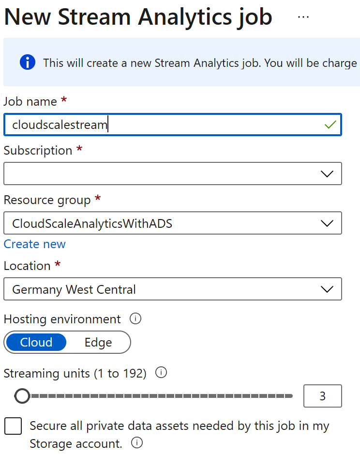
Figure 8.1 – Basic information provisioning in ASA
Please enter a job name and select the target subscription. You can either select an existing resource group or create a new one and select the data center location for your ASA job.
The Cloud hosting environment will create an ASA job in your subscription as a cloud service. If you select Edge, the ASA job will be containerized and deployed to an IoT gateway edge device.
The Streaming Units (SUs) that you can configure on this blade will determine the available compute for your streaming job.
The checkbox below all the options can trigger additional inputs where you can optionally select a storage account of your choice to store all data assets related to your ASA job. Otherwise, this data (metadata, checkpoints, job configurations, and so on) is stored with your ASA job.
- Please hit Create to start the provisioning of your configuration.
- Once your deployment is complete, you can hit Go to resource.
Now let's start examining the newly created ASA job in the next section, Implementing an ASA job.
Implementing an ASA job
ASA offers you a convenient way to create streaming analysis on a configuration basis. This means you do not need to code the environment, the engine, the connection, logging, and so on. The service will take care of all these tasks for you (to see an example, refer to the Integrating sources and Writing to sinks sections that follow). The only thing you will need to code is the analytical core of your streaming job. To ease things for you, this is done using a SQL dialect that was tailored for this task (see Understanding ASA SQL).
After the provisioning of your new resource, you are taken to the following overview blade:

Figure 8.2 – Overview blade of the ASA job
You can already see three of the most important areas of your ASA job:
- Inputs: This will show all the configured source connections available in your job.
- Outputs: This will show all the configured target connections available in your job.
- Query: This will show all the SQL statements that your job will use to process and route the data.
If you examine the navigation blade, you'll find the additional options that we are going to use and configure in the following sections. But let's move on and start creating the first source connection in the next section, Integrating sources.
Please see Figure 8.2 for an overview of how these fit together for your ASA job.
Integrating sources
The following Azure services can be configured as sources in your ASA job:
- Event Hubs: A PaaS service for caching, buffering, and processing millions of events in real time as they are sent to the Azure platform. Event Hubs is used as the "address" to which applications can send events to be further processed on the Azure platform. See the Further reading, Event Hubs section for more information.
- IoT Hub: A PaaS service specialized in IoT implementations. Optimized to scale and process billions of telemetry events, implement secure connections between devices and the Azure platform, and establish bi-directional communication between the cloud platform and devices. See the Further reading, IoT Hub section for more information.
- Blob Storage: See Chapter 3, Understanding the Data Lake Storage Layer.
- Azure Data Lake Gen2: See Chapter 3, Understanding the Data Lake Storage Layer.
For the easy setup of your first streaming job, let's use the data that you have available already in Data Lake:
- Please first navigate to your newly created ASA job. Click Inputs either on the main blade or in the Overview section.
- On the inputs list, please click Add stream input and select Blob storage/ADLS Gen2. The configuration blade will pop up from the right:
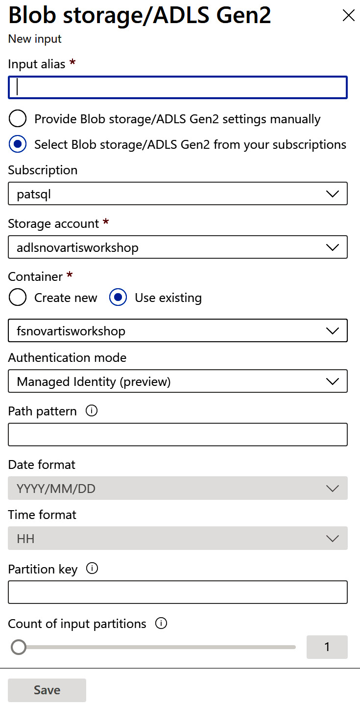
Figure 8.3 – Storage source configuration
- You can now start entering an alias for your input connection. Name it something such as airdelaystreaminginput.
If you choose to select the configuration data from your subscription, you can select from the available services from your subscription in the Subscription, Storage account, and Container fields (or create a new one). You can, of course, enter the values manually. Please select your subscription and for the storage account, select the one created in Chapter 3, Understanding the Data Lake Storage Layer. In the Container drop-down field, please select the filesystem that you created earlier.
For Authentication mode, please select Connection String. The Storage Account Key field underneath this will automatically be populated.
In the Path pattern field, you can now enter the path and name of your airdelays.csv file that will be used as streaming input. The two fields below this, Date format and Time format, can be used to resolve the date and time portions of the path pattern. Please leave them for now.
Partition key and the Count of input partitions slider can be very useful for creating input partitions to parallelize streaming jobs for higher throughput. Please leave these for now.
If you now scroll down a little, you can influence the input format in the Event serialization format field (JSON, Avro, CSV, or Other (Protobuf, XML, proprietary)) and the Delimiter (comma (,), semicolon (;), space, tab, or vertical bar(|)) drop-down box. Please select CSV and semicolon (;) and in the following Encoding field, leave it as UTF-8.
You don't need to select an event compression type (None, GZip, or Deflate).
- Please hit Save to finish and store your new input. ASA will test and then save the connection.
- To check the source, you might click on the Sample data from input button on the far right in the row of your new input to the right of the delete button (the trashcan symbol). In the following dialog, please set the date of the last modified time of your file. Otherwise, the sample won't be successful. In Duration, please set Days to 1 to ensure you find some data. Click Sample in the footer. The sampling starts and you'll be notified with a small dialog dropping in from the upper-right corner of your window. If you miss the notification, you can always check for it by clicking on the bell symbol in the top-right corner of your Azure portal. You'll find the message that your sample data is ready, and you can click to download it. If you follow the link and you're able to download the sample, your input works. Please try this as we will use this data later to test the analytical query.
Configuring Event Hubs
When you are configuring Event Hubs, you will find slightly different options to configure:
- Event Hub Namespace: The namespace is the parent collection where event hubs are grouped.
- Event Hub Name: You can use an existing one or create a new event hub from this dialog.
- Event Hub consumer group: You can use an existing one or create a new event hub consumer group. Consumer groups store the read state for the read events per group and allow you to have different groups of event consumers reading events at different times and with different rhythms. An event hub will always have a $Default consumer group.
- Authentication Mode: You can use a managed identity or connection string when you authenticate your ASA job against the event hub.
As IoT hubs are built based on event hubs, they will have a lot of similarities but differences too. Let's check them out in the next section, Configuring IoT Hub.
Configuring IoT Hub
The IoT Hub settings differ slightly from Event Hubs:
- IoT Hub: The IoT hub from which you need to read events.
- Consumer group: Consumer groups store the read state for events per group and allow you to have different groups of event consumers reading events at different times and with different rhythms. IoT Hub will always have a $Default consumer group.
- Shared access policy name: A shared access policy provides a set of permissions under a name.
- Shared access policy key: You will need to set the key according to the shared access policy name.
- Endpoint: If you select Messages, you will consume device-to-cloud messages. If you select Operations Monitoring, you will be able to read device telemetry and metadata.
But let's proceed with our example and provide a sink for our data stream in the next section, Writing to sinks.
Writing to sinks
Every ASA job writes to at least one sink. Let's examine your options here.
The following services can be used as sinks in an ASA job. Please find the different properties in this list:
- Event Hubs.
- SQL databases: Azure SQL Database tables as sinks. Can come in very handy when used with reporting.
- Blob storage/Azure Data Lake Storage Gen2: See Chapter 3, Understanding the Data Lake Storage Layer.
- Table storage: Uses a storage account table storage.
- Service Bus topic: Azure Service Bus offers messaging services for asynchronous messaging. A Service Bus topic offers a publish and subscribe pattern for a service bus and can be used as a sink from ASA. Please find more details in the Further reading section.
- Service Bus queue: In comparison to a Service Bus topic, the queue offers a first-in/first-out messaging queue for one or more, in this case, "competing" consumers. Please find more details in the Further reading, Service Bus section.
- Cosmos DB: NoSQL component in Azure.
- Power BI: The Microsoft reporting and dashboarding solution. Power BI offers the option of streaming datasets that can catch ASA streams. You will need to have a PowerBI.com account and you will need to first authenticate with the PowerBI.com service.
- Data Lake Storage Gen1: Legacy Azure Data Lake Storage technology is provided for backward compatibility.
- Azure Functions: Compute component for serverless functions.
- Azure Synapse Analytics: See Chapter 4, Understanding Synapse SQL Pools and SQL Options.
For detailed overviews, please check the Further reading, Sinks section.
Please proceed now to set up a sink according to the input that you have created to a target folder in your Data Lake Storage. Maybe name it something such as airdelaystreamingtarget.
Understanding ASA SQL
The main processing in your ASA job will be done using SQL to implement the analytical rules you want to apply to your incoming data.
Compared to data warehouse batch-oriented processing, stream processing observes a constantly delivered chain of events. The processing, therefore, will need different approaches as you will, for example, aggregate values over a certain recurring time frame. This is called windowing. The ASA SQL dialect implements a collection of windowing functions that will support you in doing this.
But before we dive into the magic of windowing functions and ASA, let's first finish our basic ASA job and kick it:
- Please select Query from either the navigation blade or the Overview blade and select Edit query:
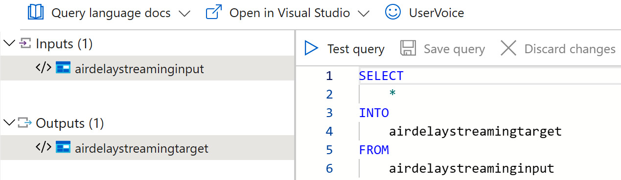
Figure 8.4 – ASA query editor
- In the editor, please enter your ASA query. Please replace the displayed query with the following:
SELECT
*
INTO
airdelaystreamingtarget
FROM
airdelaystreaminginput
- Of course, please check the two aliases and if you have named them differently, please use the names that you have used.
- Once you're done adjusting the query, you can click Save query in the editor window. There is the option to test your query with some sample data that you can get from the source. We're going to have a look at this later.
- For now, please save the query and return to the Overview blade of your ASA job. You can find some controls in the upper area of the overview:

Figure 8.5 – Run controls for ASA jobs
- Please press start and kick your ASA job for the first time. From the right, the Start job dialog pops up:

Figure 8.6 – Start job dialog
- Please use Custom and select the creation date of your source file in the Start time fields. Click Start in the footer when you are ready.
If you use Now, the job would expect events in your source with a date and time equal to or after the starting time.
When last stopped will resume the job from where it was stopped and will pick up the event right after the last-saved timestamp.
ASA will internally store the state of your job to enable you to pick up where you left off.
Once you have started your job, it will take some seconds before it kicks off. You can see a small running bar beneath the bell symbol, the notification symbol, in the upper-right ribbon of your Azure portal:
Figure 8.7 – Notification symbol in the Azure portal
If you click the notification button, you will find all kinds of messages related to your Azure environment:
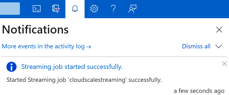
Figure 8.8 – Notifications in your Azure subscription
Once your job is running, you will be presented with some statistics about it in the Overview window. Input Events, Output Events, Runtime Errors, and SU Utilization are shown in two charts:
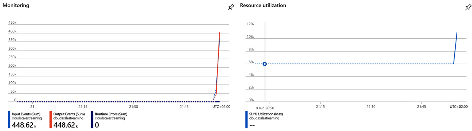
Figure 8.9 – Job statistics
Please proceed now to your target folder in Data Lake and check the output of your job. You should have created a file with all the columns that came from the source file. If you scroll to the far-right end of the file, you will find additional information added: EventProcessedUtcTime, PartitionID, BlobName, and BlobLastModifiedUtcTime.
If there is no data, you can check the graph shown in Figure 8.9 on the left to see whether there have been some runtime errors. The notification list (see Figure 8.8) will list errors if they occur. So, if your job was not started successfully, you will find a message there.
In this case, please go through the settings of your input and output and maybe even check the query. Sometimes the input and output get mixed up.
Understanding windowing
As mentioned previously, stream computing adds additional options to your processing logic. In a batch-oriented world, you have a certain input dataset. It can be read, filtered, and aggregated in one go and is then written to the target.
In a streaming world, the input keeps flowing into your system. It has a start but not necessarily an ending date and time. Therefore, we need to observe certain time frames. Maybe the analogy of a traffic census can help with understanding the challenge:

Figure 8.10 – Traffic census windowing example
You are recording the information for the census and will count cars and their types and colors passing by for an agreed amount of time. This time frame constitutes a window.
Now, this is a very basic example of a window. There can be quite a few differences when we think about the time frames and possible overlaps that windows can have.
Understanding tumbling windows
Maybe you want to count your cars every 10 minutes. The 10 minutes will then be your window. If you don't overlap the windows and want to keep the window time frame fixed, you are talking about a tumbling window:
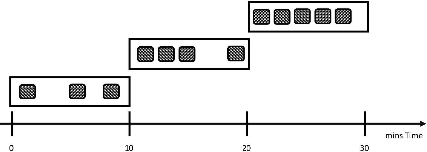
Figure 8.11 – Tumbling window
Later, you'll find some code examples about windowing functions in the Using window functions in your SQL section.
Understanding hopping windows
If you need to analyze overlapping time frames – let's say for every 2 minutes you want to count the cars that passed by in the last 4 minutes – you are looking at so-called hopping windows:
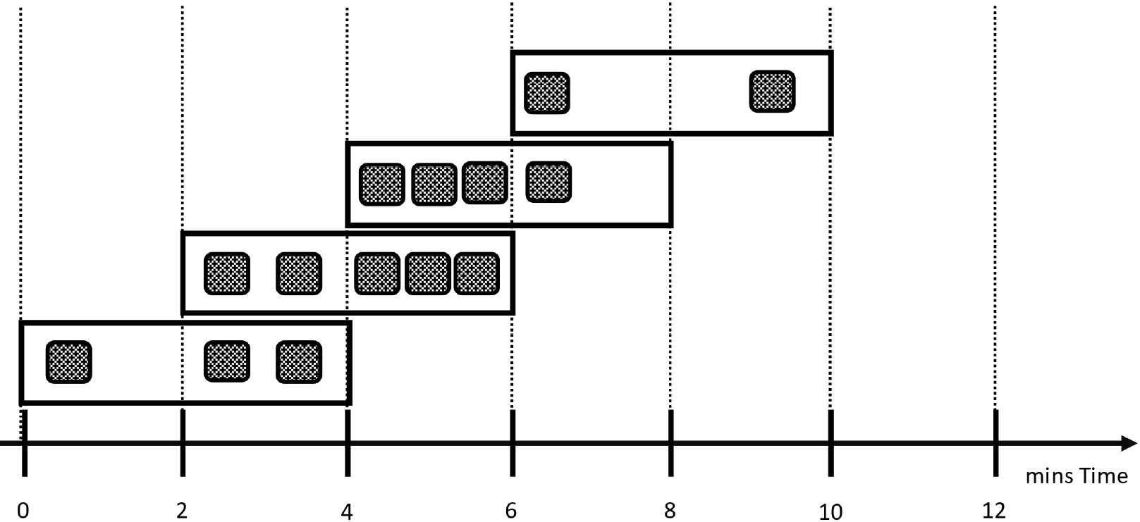
Figure 8.12 – Hopping windows
Understanding session windows
Maybe you need to analyze a set of events that are close in time to each other. Let's say you want to count cars that drive 30 seconds behind each other. In this case, your session starts when the first two cars appear that are 30 seconds or less behind each other. The session will only end when there has been no car following the last one for 30 seconds or when the duration configured to the function has been reached. The next session will then follow the same rules but doesn't need to last the same amount of time as the first one. Session windows might produce very different time frames for the session:

Figure 8.13 – Session windows
Understanding sliding windows
On the one hand, sliding windows consider all the possible windows of a given length. As this might lead to an infinite number of windows, ASA will only return the windows that actually caught a change.
On the other hand, sliding windows add another dimension to the analysis. You can add conditions to the groups that you are analyzing. Let's say you want to know whether there have been more than five cars per type in the last 10 minutes. To extract this information from your stream, you will use a sliding window:
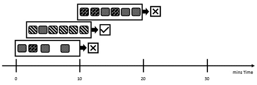
Figure 8.14 – Sliding windows
The example in Figure 8.14 shows that for the second window, the condition of five cars per type in the last 10 minutes has been satisfied. This condition is false for the two other windows.
Later, you'll find some code examples about window functions in the Using window functions in your SQL section.
Understanding snapshot windows
There is yet another type of window that checks exactly one point in time:
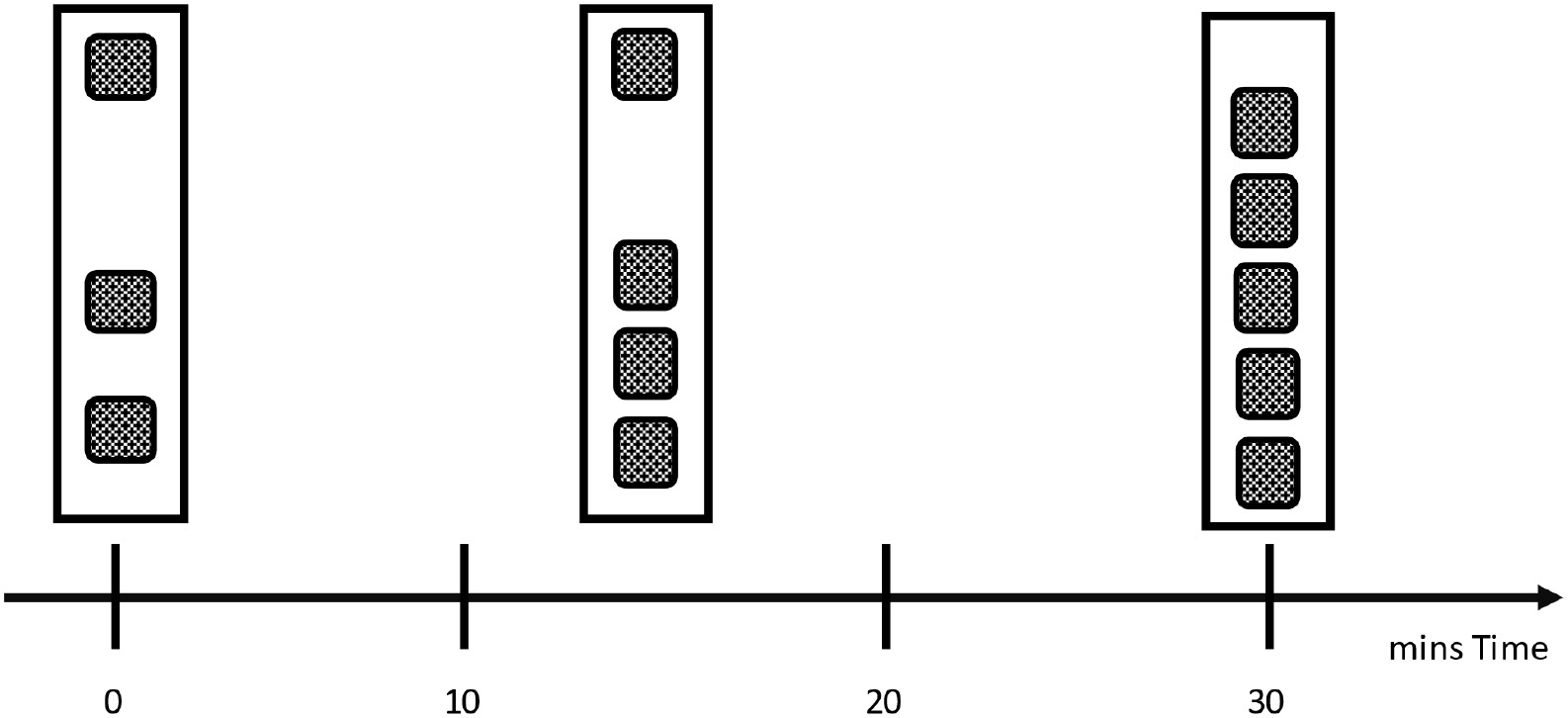
Figure 8.15 – Snapshot window
Using window functions in your SQL
To be able to use windowing functions with your stream, you would need a timestamp coming from your input. In the SQL statement, you will flag this timestamp with the TIMESTAMP BY statement.
Windowing functions are aggregate functions. This means they are always implemented in the GROUP BY clause of your SQL statement:
- For example, the tumbling window from Figure 8.11 would be implemented as follows:
SELECT
CensusStation,
COUNT(*) as Amount
FROM
Cartraffic
TIMESTAMP BY
ObservedT
GROUP BY
CensusStation,
TUMBLINGWINDOW(minute, 10)
- The hopping window from Figure 8.12 would be implemented like this:
SELECT
CensusStation,
COUNT(*) as Amount
FROM
Cartraffic
TIMESTAMP BY
ObservedT
GROUP BY
CensusStation,
HOPPINGWINDOW(minute, 4, 2)
- If you want to implement a session window, you would again need three parameters set:
SELECT
CensusStation,
COUNT(*) as Amount
FROM
Cartraffic
TIMESTAMP BY
ObservedT
GROUP BY
CensusStation,
SESSIONWINDOW(seconds, 30, 180)
In this case, we have added a maximum 3-minute duration (180 seconds) for the observation.
- The sliding window will need another SQL clause that we implement to filter the grouped results – the HAVING clause:
SELECT
CensusStation,
CarColor,
COUNT(*) as Amount
FROM
Cartraffic
TIMESTAMP BY
ObservedT
GROUP BY
CensusStation,
CarColor,
SLIDINGWINDOW(minute, 10)
HAVING COUNT(*) > 5
- The snapshot window, finally, is not using a particular window function. It just groups by a timestamp that you want to explore:
SELECT
CensusStation,
COUNT(*) as Amount
FROM
Cartraffic
TIMESTAMP BY
ObservedT
GROUP BY
CensusStation,
System.Timestamp()
Please check the Further reading section for a deep dive into the documentation.
For an example that runs a small app and sends data to an event hub from where you can consume a real stream, please check the GitHub repo.
Delivering to more than one output
The SQL query of your ASA job is not tied to one output only. You can use it to deliver data from your input to several different outputs using different queries with different granularities.
Think of it as a configurable routing mechanism where you create the suitable datasets for any target that you need to deliver to. Maybe you want to land every event in its raw form into Data Lake. This is often referred to as the cold path.
At the same time, you need to display some aggregated numbers on a Power BI dashboard, which is the hot path.
Additionally, you might need to process the input data using a machine learning model to detect fraud or predict machine failure. The results of such a prediction and only the results need to be sent to another event hub where it will be used to trigger an alert in another system. This is another branch of the hot path.
All these routes can be set up in your ASA job query. Let's use some of the query examples from previously and put them together. You don't need to add a terminator between the queries; just put them behind each other. Let's stick to the assumptions just formulated.
First, we just drop every event into a data lake, then the second query adds a tumbling window over 10 minutes (just like previously) and writes the aggregated numbers to a Power BI streaming dataset that feeds a dashboard visual.
The example tumbling window from Figure 8.11 would be implemented as follows:
SELECT
CensusStation,
COUNT(*) as Amount
INTO
POWERDISTREAMINGDS
FROM
Cartraffic TIMESTAMP BY ObservedT
GROUP BY
CensusStation,
TUMBLINGWINDOW(minute, 10)
Have you managed to implement a window function in your ASA job?
Adding reference data to your query
In many cases, the data coming from your input will not satisfy the needs of your required analysis. You will need to add data from other sources, such as a master data database, for example, or files that contain data that you need to enrich the query to create the information needed in your analysis.
In ASA inputs, you can add reference data as inputs that can be additionally used to be joined into your analytical queries. These inputs can be derived from the following:
- Blob storage or Data Lake Gen2
- SQL databases
The references are literally joined into the query using a JOIN clause and you have the option to use an inner or left outer join.
If we follow our example from the census station and maybe try to add the fuel type and potential average air pollution from a car type file, we could, for example, derive the average air pollution emitted at the census station:
SELECT
t1.Cartype,
SUM(t2.mgNOx/60) as SumNOx
FROM
Cartraffic as t1 TIMESTAMPED BY ObservedT
JOIN
CarStats as t2
ON
t1.Cartype = t2.Cartype
GROUP BY
t1.Cartype,
TUMBLINGWINDOW(minute, 10)
Please check the Further reading, Reference data section for additional information on how to use reference data and join it to your input.
Using joins for different inputs
Joins are not just used to add reference data to your stream. You can also use the JOIN clause of the ASA SQL dialect to join two inputs together. You will need a TIMESTAMPED BY statement for each of the sources to synchronize the stream and sort the right events together. You won't need to explicitly add an ON clause to your statement to bring the two inputs together on the timestamp unless you need additional join logic on attributes of the two streams.
Please check the Further reading, Joins section for information about joining inputs. You might also want to examine the topic of temporal joins, such as joins with DATEDIFFS and temporal analytical functions such as FIRST, LAST, or LAG with LIMIT DURATION.
Implementing pattern recognition
ASA SQL implements a function that might come in handy when you want to find and react to patterns hidden in your input data. MATCH_RECOGNIZE enables you to implement even complex regular expression patterns and use them with your incoming data stream.
MATCH_RECOGNIZE will support you in recognizing patterns within a configurable time frame and over several rows when you want to find a repeating pattern in your data.
Let's examine a simple example for a pattern matching in our census case for car colors to display the usage. In this case, you would produce outputs when you find two red cars within 1 minute in your input stream:
SELECT
*
INTO
DataLakeOutput
FROM
Cartraffic TIMESTAMPED BY ObservedT
MATCH_RECOGNIZE (
LIMIT DURATION(minute, 1)
PARTITION BY CensusStation
MEASURES
Last(RedColor.CensusStation) AS CensusStation,
Last(RedColor.CensusTracker) AS CensusTracker,
Last(RedColor.CarType) AS RedColorCartype
AFTER MATCH SKIP TO NEXT ROW
PATTERN (Red{2,} Blue*)
DEFINE
Red AS Red.Color = 'Red'
Blue AS Blue.Color = 'Blue'
) AS MATCHINGSTREAM
You will find a link to the MATCH_RECOGNIZE function documentation in the Further reading, MATCH_RECOGNIZE section.
There is also a link to a great list of typical queries and usage patterns in ASA for you in the Further reading, Typical query usage section.
Adding functions to your ASA job
If you examine the Job topology section in the navigator of your ASA job, you will find the Functions entry. You can implement additional functionality for your ASA job.
Maybe you want to decode the payload of your incoming event because it is binary-coded following a special pattern. Another option would be to add an Azure Machine Learning service or a model from Azure Machine Learning Studio to score your input or to predict any circumstance based on incoming data.
Functions can be implemented from the following:
- The Azure Machine Learning service: You can create a function within Azure Machine Learning Studio and deploy it as a web service.
- Azure Machine Learning Studio: You can use Azure Machine Learning (classic) and create a callable web service that will be implemented here.
- JavaScript user-defined functions (UDFs): You can add your own JavaScript UDF code to your ASA job in this way. An editor window will open where you can enter your function.
- JavaScript user-defined aggregators (UDAs): You can add a custom JavaScript UDA using this option. An editor will open where you can add and edit your custom aggregation function.
As a fifth option, you can develop C# user-defined functions with Visual Studio Code and use them in your SQL query. With Visual Studio Code, you can then deploy the whole setup to your ASA job.
Please find details about implementing and using functions in the Further reading, Functions section.
Understanding streaming units
ASA does its processing in memory. Therefore, you want to make sure your job is always equipped with the right amount of SUs. These represent the compute resources of ASA and form a combined factor of CPU and memory.
If you check the chart on the right in Figure 8.9, you will find a percentage of memory utilization of SUs of your ASA job. This is quite an important one to observe in your ASA job. You want to keep the utilization percentage of your ASA job always below 80%. If your job runs out of memory, it will fail. You won't see the CPU consumption here, so you might want your SUs to be a little bit ahead of your jobs. Maybe you want to set an alert to be notified when your job exceeds a threshold on its way up over 80%.
As a rule of thumb, you would start with six SUs and observe the performance of your job. Don't partition from the beginning! You need to experiment with your data, the complexity and number of steps of your queries, and the number of partitions of your job to balance the right SU settings. Please find a link to more information in the Microsoft documentation about the limits and how to calculate a baseline setting for SUs for your job in the Further reading, Optimizing Azure Stream Analytics section.
Partitioning
Adding partitions to your ASA job will help improve the performance, especially when your input data is already partitioned. When you examine the partition key in the source settings (see the Integrating sources section), you can select the attribute from your source and determine the number of partitions for your job. If you manage to synchronize your input and output partitions, this can have a big impact on the throughput of your job.
Additionally, you have the option to use the PARTITION BY statement in your query logic to even synchronize the job logic with the input and output.
Synchronizing your partitions means that you need to have the same amount of input partitions as you have output partitions. When your job writes to Azure Storage, the storage account will inherit the partition settings. Please check the Further reading, Optimizing Azure Stream Analytics section for more information on partitioning.
Resuming your job
As mentioned already, ASA will always store checkpoint information internally to be able to resume your jobs in the case of failure. Functions that support a so-called stateful query logic in temporal elements are as follows:
- The window functions in the GROUP BY clause
- Temporal joins
- Temporal analytical functions
If your job needs recovery, it will be able to restart from the last available checkpoint.
Note
There are rare cases when ASA will not be able to store checkpoints for a job recovery. When Microsoft needs to update the service where your ASA job is running, checkpoint data is not stored. You will need to additionally take care of your input data and its retention time.
As a rule of thumb, you might minimally have a retention time in your source data that fits the window size of your ASA job. Please find more information about job recovery and replay times in the Further reading section.
Using Structured Streaming with Spark
If you are more the kind of developer that loves to code and you are a fan of Spark, maybe you want to have a look at Structured Streaming with Spark. This might be an interesting alternative for you.
Spark clusters are a widely used engine to implement streaming analytics using one of the available programming languages, such as Python or Scala. With the massive scalability of Spark clusters in Azure services such as Synapse or Databricks, you will be able to implement an environment that can grow with your needs and deliver the necessary performance.
Next to performance, there is the extensibility of Spark clusters that is a factor to consider. You will be able to combine streaming algorithms with the capabilities of Spark and programming languages such as Python (PySpark), Scala, or R.
Take Kafka as input for your streaming analysis, for example. Kafka is an event streaming platform that is quite widely used. ASA does not yet offer a connector to Kafka; therefore, you will need to find another way. Spark offers a Kafka library that you can implement into your streaming solution.
Spark too offers windowing functions and the capability to write to many sinks, Azure Data Lake Storage included.
If you want to read more about Structured Streaming with Spark, please refer to the link in the Further reading, Structured Streaming with Spark section.
Security in your streaming solution
Secure access to sources and sinks in your solution is paramount. There are some considerations that you might want to go through when implementing a streaming solution with ASA.
Connecting to sources and sinks
If you examine the Integrating sources and Writing to sinks sections, you will find the authentication mode in the list of the connectors in almost every one except Event Hubs and IoT Hub, where you would use key and connection strings to connect.
Implementing authentication with either service users and passwords or managed identities will already create very secure access into your sources and sinks. Azure Active Directory implements a multitude of security measures to eliminate the possibility for attackers to break into your solution.
With the use of managed identities, you are implementing a service principal. This is a kind of Azure user that can only be used with Azure services. You can compare them to the on-premises service users that can be configured to only be used with a service and not, for example, for an interactive session.
Please find a link to an overview about Azure managed identities in the Further reading, Managed identities section.
Understanding ASA clusters
ASA clusters are an additional offering when it comes to the Azure Stream PaaS component.
With ASA clusters, you can create a shared environment for ASA jobs that can be used by several developers from your company.
An ASA cluster can scale to 216 SUs in comparison to the 192 of single ASA jobs. But the more important option of clusters in comparison to single jobs is the capability to connect to Virtual Networks (vNets) using private endpoints. This means when you are implementing network security in your Azure tenant and plan to "hide" your resources within vNets, you will need to use an ASA cluster as single ASA jobs can't be used with private endpoints.
You will find a link to an introduction to ASA clusters in the Further reading, ASA clusters section.
Monitoring your streaming solution
As seen in Figure 8.9, you can see some information already on the Overview page of your ASA job. If you navigate to the Monitoring section of your ASA job, you can get further insights into your job.
In the Logs section, for example, you are presented with a list of predefined queries that will produce insights into all kinds of errors that can occur when you are running your ASA job:
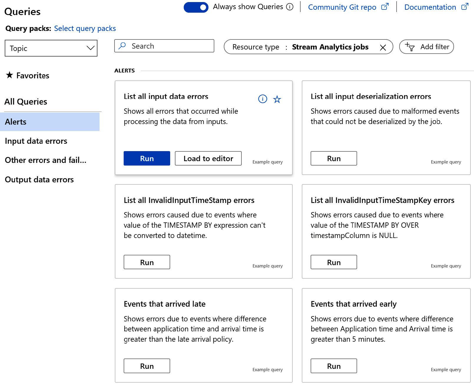
Figure 8.16 – Available error queries in the Logs section
If you proceed to Metrics, you are taken to a chart editor where you can select from the available ASA metrics:
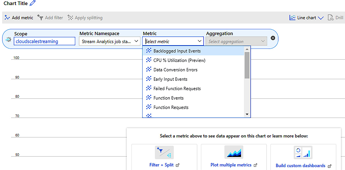
Figure 8.17 – ASA metrics view
You have metrics such as backlogged input events, data conversion errors, early input events, and failed function requests. This section will give you a deep insight into your ASA job.
If you want to set up alerts for your ASA job, such as the SU percentage utilization, for example (remember the Understanding streaming units section), this is the place to do so.
Let's implement an alert to be sent when the SU percentage utilization hits 70%:
- In the Alert rules section, hit + New alert rule. In the following blade, you will find your ASA job already selected in the Resource section.
- In the Condition section, please click Add condition, and in the following dialog, select SU % utilization as the signal name.
- In the Configure signal logic dialog, scroll to the bottom and enter 70 in the Threshold value field, and hit Done. The condition will show in the list.
- Next, you can set up an action group in the Actions section. Please check Application Insights Smart Detection and hit Select. The action group name will show.
Finally, name your alert in the Alert rule details section. You can set a name and a description, select a resource group from your subscription, and configure a severity for your rule. Once you have checked the box below Enable alert rule upon creation, your rule will become active when you create it:
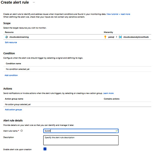
Figure 8.18 – Creating an alert rule
You will need to click Manage Alert rules to see a list of your implemented rules. From there, you can control your rules and manage them.
Using Azure Monitor
ASA, like all the other PaaS components on Azure, integrates with Azure Monitor. You can configure ASA to deliver telemetry to Azure Monitor. By doing so, you will be able to put your streaming analysis telemetry into correlation with other components of your solution. You can therefore produce insights in a wider focus.
For example, you might want to correlate your ASA insights with the logs of your Event Hubs and Azure Data Lake Storage, which may act as input and output for your ASA job.
In the Monitoring section, you can do the correlation in the diagnostic settings. If you enable them, you can send log details from Execution, Authoring, and All Metrics.
You can select to send the details to your Log Analytics workspace, archive to a storage account, and/or stream to an event hub.
Please find information about Azure Monitor in the Further reading, Azure Monitor section.
Summary
In this chapter, you have learned how to provision an ASA job. You have seen how to connect to sources and sinks and how to use them as inputs and outputs. You have also learned about ASA SQL and its windowing functions.
Furthermore, you have seen that ASA SQL queries can route data from the input to different outputs, creating different granularities. You have examined the capabilities to add reference data to your queries and how to add further functionality such as user-defined functions and machine learning using functions.
Finally, we have talked about SUs, the performance metrics of ASA, and how partitioning will help you to improve performance. You have examined security questions and have learned about monitoring. If all the features of ASA do not deliver on your requirements, there are additional technologies available on Azure, such as Spark clusters in Synapse or Databricks that can be used to implement streaming.
We have touched on the topic of machine learning now already several times. If you are interested in the available capabilities on Azure, please proceed to Chapter 9, Integrating Azure Cognitive Services and Machine Learning.
Further reading
- Event Hubs: https://docs.microsoft.com/en-us/azure/event-hubs/event-hubs-about
- IoT Hub: https://docs.microsoft.com/en-us/azure/iot-hub/about-iot-hub
- Service Bus: https://docs.microsoft.com/en-us/azure/service-bus-messaging/service-bus-queues-topics-subscriptions
- Sinks: https://docs.microsoft.com/en-us/azure/stream-analytics/stream-analytics-define-outputs
- Optimizing Azure Stream Analytics: https://docs.microsoft.com/en-us/azure/stream-analytics/stream-analytics-parallelization
- Window functions: https://docs.microsoft.com/en-us/stream-analytics-query/windows-azure-stream-analytics
- Job recovery: https://docs.microsoft.com/en-us/azure/stream-analytics/stream-analytics-concepts-checkpoint-replay
- Reference data: https://docs.microsoft.com/en-us/stream-analytics-query/reference-data-join-azure-stream-analytics
- Joins: https://docs.microsoft.com/en-us/stream-analytics-query/join-azure-stream-analytics
- MATCH_RECOGNIZE: https://docs.microsoft.com/en-us/stream-analytics-query/match-recognize-stream-analytics
- Typical query usage: https://docs.microsoft.com/en-us/azure/stream-analytics/stream-analytics-stream-analytics-query-patterns
- Functions:
Functions overview: https://docs.microsoft.com/en-us/azure/stream-analytics/functions-overview
C# user-defined functions: https://docs.microsoft.com/en-us/azure/stream-analytics/stream-analytics-edge-csharp-udf-methods
- ASA clusters: https://docs.microsoft.com/en-us/azure/stream-analytics/cluster-overview
- Managed identities: https://docs.microsoft.com/en-us/azure/active-directory/managed-identities-azure-resources/
- Structured Streaming with Spark: https://docs.microsoft.com/en-us/azure/architecture/reference-architectures/data/stream-processing-databricks
- Azure Monitor: https://docs.microsoft.com/en-us/azure/azure-monitor/overview