
5
General Clustering Techniques
5.1 Brief Overview of Clustering
As an exploratory tool, clustering techniques are frequently used as a means of identifying features in a data set, such as sets or subsets of observations with certain common (known or unknown) characteristics. The aim is to group observations into clusters (also called classes, or groups, or categories, etc.) that are internally as homogeneously as possible and as heterogeneous as possible across clusters. In this sense, the methods can be powerful tools in an initial data analysis, as a precursor to more detailed in‐depth analyses.
However, the plethora of available methods can be both a strength and a weakness, since methods can vary in what specific aspects are important to that methodology, and since not all methods give the same answers on the same data set. Even then a given method can produce varying results depending on the underlying metrics used in its applications. For example, if a clustering algorithm is based on distance/dissimilarity measures, we have seen from Chapters 3 and that different measures can have different values for the same data set. While not always so, often the distances used are Euclidean distances (see Eq. (3.1.8)) or other Minkowski distances such as the city block distance. Just as no one distance measure is universally preferred, so it is that no one clustering method is generally preferred. Hence, all give differing results; all have their strengths and weaknesses, depending on features of the data themselves and on the circumstances.
In this chapter, we give a very brief description of some fundamental clustering methods and principles, primarily as these relate to classical data sets. How these translate into detailed algorithms, descriptions, and applications methodology for symbolic data is deferred to relevant later chapters. In particular, we discuss clustering as partitioning methods in section 5.2 (with the treatment for symbolic data in Chapter 6 ) and hierarchical methods in section 5.3 (and in Chapter 7 for divisive clustering and Chapter 8 for agglomerative hierarchies for symbolic data). Illustrative examples are provided in section 5.4, where some of these differing methods are applied to the same data set, along with an example using simulated data to highlight how classically‐based methods ignore the internal variations inherent to symbolic observations. The chapter ends with a quick look at other issues in section 5.5. While their interest and focus is specifically targeted at the marketing world, Punj and Stewart (1983) provide a nice overview of the then available different clustering methods, including strengths and weaknesses, when dealing with classical realizations; Kuo et al. (2002) add updates to that review. Jain et al. (1999) and Gordon (1999) provide overall broad perspectives, mostly in connection with classical data but do include some aspects of symbolic data.
We have ![]() observations
observations ![]() with realizations described by
with realizations described by ![]() ,
, ![]() , in
, in ![]() ‐dimensional space
‐dimensional space ![]() . In this chapter, realizations can be classical or symbolic‐valued.
. In this chapter, realizations can be classical or symbolic‐valued.
5.2 Partitioning
Partitioning methods divide the data set of observations ![]() into non‐hierarchical, i.e., not nested, clusters. There are many methods available, and they cover the gamut of unsupervised or supervised, agglomerative or divisive, and monothetic or polythetic methodologies. Lance and Williams (1967a) provide a good general introduction to the principles of partitions. Partitioning algorithms typically use the data as units (in
into non‐hierarchical, i.e., not nested, clusters. There are many methods available, and they cover the gamut of unsupervised or supervised, agglomerative or divisive, and monothetic or polythetic methodologies. Lance and Williams (1967a) provide a good general introduction to the principles of partitions. Partitioning algorithms typically use the data as units (in ![]() ‐means type methods) or distances (in
‐means type methods) or distances (in ![]() ‐medoids type methods) for clustering purposes.
‐medoids type methods) for clustering purposes.
The basic partitioning method has essentially the following steps:
- Establish an initial partition of a pre‐specified number of clusters
 .
. - Determine classification criteria.
- Determine a reallocation process by which each observation in
 can be reassigned iteratively to a new cluster according to how the classification criteria are satisfied; this includes reassignment to its current cluster.
 - Determine a stopping criterion.
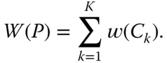
The convergence of the basic partitioning method can be formalized as follows. Let ![]() be a quality criterion defined on any partition
be a quality criterion defined on any partition ![]() of the initial population, and let
of the initial population, and let ![]() be defined as the quality criterion on the cluster
be defined as the quality criterion on the cluster ![]() ,
, ![]() , with
, with
Both ![]() and
and ![]() have positive values, with the internal variation decreasing as the homogeneity increases so that the quality of the clusters increases. At the
have positive values, with the internal variation decreasing as the homogeneity increases so that the quality of the clusters increases. At the ![]() th iteration, we start with the partition
th iteration, we start with the partition ![]() . One observation from cluster
. One observation from cluster ![]() , say, is reallocated to another cluster
, say, is reallocated to another cluster ![]() , say, so that the new partition
, say, so that the new partition ![]() decreases the overall criterion
decreases the overall criterion ![]() . Hence, in this manner, at each step
. Hence, in this manner, at each step ![]() decreases and converges since
decreases and converges since ![]() .
.
There are many suggestions in the literature as to how the initial clusters might be formed. Some start with ![]() seeds, others with
seeds, others with ![]() clusters. Of those that use seeds, representative methods, summarized by Anderberg (1973) and Cormack (1971), include:
clusters. Of those that use seeds, representative methods, summarized by Anderberg (1973) and Cormack (1971), include:
- Select any
 observations from
  subjectively.
 - Randomly select
 observations from
  .
. - Calculate the centroid (defined, e.g., as the mean of the observation values by variable) of
 as the first seed and then select further seeds as those observations that are at least some pre‐specified distance from all previously selected seeds.
 - Choose the first
 observations in
  .
. - Select every
 th observation in
  .
.
For those methods that start with initial partitions, Anderberg's (1973) summary includes:
- Randomly allocate the
 observations in
  into
into  clusters.
 - Use the results of a hierarchy clustering.
- Seek the advice of experts in the field.
Other methods introduce “representative/supplementary” data as seeds. We observe that different initial clusters can lead to different final clusters, especially when, as is often the case, the algorithm used is based on minimizing an error sum of squares as these methods can converge to local minima instead of global minima. Indeed, it is not possible to guarantee that a global minima is attained unless all possible partitions are explored, which detail is essentially impossible given the very large number of possible clusters. It can be shown that the number of possible ![]() clusters from
clusters from ![]() observations is the Stirling number of the second kind,
observations is the Stirling number of the second kind,

Thus, for example, suppose ![]() . Then, when
. Then, when ![]() ,
, ![]() , and when
, and when ![]() ,
, ![]() .
.
The most frequently used partitioning method is the so‐called ![]() ‐means algorithm and its variants introduced by Forgy (1965), MacQueen (1967), and Wishart (1969). The method calculates the mean vector, or centroid, value for each of the
‐means algorithm and its variants introduced by Forgy (1965), MacQueen (1967), and Wishart (1969). The method calculates the mean vector, or centroid, value for each of the ![]() clusters. Then, the iterative reallocation step involves moving each observation, one at a time, to that cluster whose centroid value is closest; this includes the possibility that the current cluster is “best” for a given observation. When, as is usually the case, a Euclidean distance (see Eq. (3.1.8)) is used to measure the distance between an observation and the
clusters. Then, the iterative reallocation step involves moving each observation, one at a time, to that cluster whose centroid value is closest; this includes the possibility that the current cluster is “best” for a given observation. When, as is usually the case, a Euclidean distance (see Eq. (3.1.8)) is used to measure the distance between an observation and the ![]() means, this implicitly minimizes the variance within each cluster. Forgy's method is non‐adaptive in that it recalculates the mean vectors after a complete round (or pass) on all observations has been made in the reallocation step. In contrast, MacQueen's (1967) approach is adaptive since it recalculates the centroid values after each individual observation has been reassigned during the reallocation step. Another distinction is that Forgy continues the reiteration of these steps (of calculating the centroids and then passing through all observations at the reallocation step) until convergence, defined as when no further changes in the cluster compositions occur. On the other hand, MacQueen stops after the second iteration.
means, this implicitly minimizes the variance within each cluster. Forgy's method is non‐adaptive in that it recalculates the mean vectors after a complete round (or pass) on all observations has been made in the reallocation step. In contrast, MacQueen's (1967) approach is adaptive since it recalculates the centroid values after each individual observation has been reassigned during the reallocation step. Another distinction is that Forgy continues the reiteration of these steps (of calculating the centroids and then passing through all observations at the reallocation step) until convergence, defined as when no further changes in the cluster compositions occur. On the other hand, MacQueen stops after the second iteration.
These ![]() ‐means methods have the desirable feature that they converge rapidly. Both methods have piece‐wise linear boundaries between the final cluster. This is not necessarily so for symbolic data, since, for example, interval data produce observations that are hypercubes in
‐means methods have the desirable feature that they converge rapidly. Both methods have piece‐wise linear boundaries between the final cluster. This is not necessarily so for symbolic data, since, for example, interval data produce observations that are hypercubes in ![]() rather than the points of classically valued observations; however, some equivalent “linearity” concept would prevail. Another variant uses a so‐called forcing pass which tests out every observation in some other cluster in an effort to avoid being trapped in a local minima, a short‐coming byproduct of these methods (see Friedman and Rubin (1967)). This approach requires an accommodation for changing the number of clusters
rather than the points of classically valued observations; however, some equivalent “linearity” concept would prevail. Another variant uses a so‐called forcing pass which tests out every observation in some other cluster in an effort to avoid being trapped in a local minima, a short‐coming byproduct of these methods (see Friedman and Rubin (1967)). This approach requires an accommodation for changing the number of clusters ![]() . This is particularly advantageous when outliers exist in the data set. Other variants involve rules as to when the iteration process stops, when, if at all, a reallocation process is implemented on the final set of clusters, and so on. Overall then, no completely satisfactory method exists. A summary of some of the many variants of the
. This is particularly advantageous when outliers exist in the data set. Other variants involve rules as to when the iteration process stops, when, if at all, a reallocation process is implemented on the final set of clusters, and so on. Overall then, no completely satisfactory method exists. A summary of some of the many variants of the ![]() ‐means approach is in Jain (2010).
‐means approach is in Jain (2010).
While the criteria driving the reallocation step can vary from one approach to another, how this is implemented also changes from one algorithm to another. Typically though, this is achieved by a hill‐climbing steepest descent method or a gradient method such as is associated with Newton–Raphson techniques. This ![]() ‐means method is now a standard method widely used and available in many computer packages.
‐means method is now a standard method widely used and available in many computer packages.
A more general partitioning method is the “dynamical clustering” method. This method is based on a “representation function” (![]() ) of any partition with
) of any partition with ![]() . This associates a representation
. This associates a representation ![]() with each cluster
with each cluster ![]() of the partition
of the partition ![]() . Then, given
. Then, given ![]() , an allocation function
, an allocation function ![]() with
with ![]() associates a cluster
associates a cluster ![]() of a new partition
of a new partition ![]() with each representation of
with each representation of ![]() of
of ![]() . For example, for the case of a representation by density functions (
. For example, for the case of a representation by density functions (![]() , each individual
, each individual ![]() is then allocated to the cluster
is then allocated to the cluster ![]() if
if ![]() for this individual. In the case of representation by regression, each individual is allocated to the cluster
for this individual. In the case of representation by regression, each individual is allocated to the cluster ![]() if this individual has the best fit to the regression
if this individual has the best fit to the regression ![]() , etc. By alternating the use of these
, etc. By alternating the use of these ![]() and
and ![]() functions, the method converges.
functions, the method converges.
More formally, starting with the partition ![]() of the population
of the population ![]() , the representation function
, the representation function ![]() produces a vector of representation
produces a vector of representation ![]() such that
such that ![]() . Then, the allocation function
. Then, the allocation function ![]() produces a new partition
produces a new partition ![]() such that
such that ![]() . Eq. 5.2.1 can be generalized to
. Eq. 5.2.1 can be generalized to
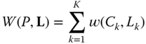
where ![]() is a measure of the “fit” between each cluster
is a measure of the “fit” between each cluster ![]() and its representation
and its representation ![]() and where
and where ![]() decreases as the fit increases. For example, if
decreases as the fit increases. For example, if ![]() is a distribution function, then
is a distribution function, then ![]() could be the inverse of the likelihood of the cluster
could be the inverse of the likelihood of the cluster ![]() for distribution
for distribution ![]() .
.
That convergence of this more general dynamical clustering partitioning method pertains can be proved as follows. Suppose at the ![]() th iteration we have the partition
th iteration we have the partition ![]() and suppose the representation vector is
and suppose the representation vector is ![]() , and let
, and let ![]() be the quality measure on
be the quality measure on ![]() at this
at this ![]() th iteration. First, by the reallocation of each individual belonging to a cluster
th iteration. First, by the reallocation of each individual belonging to a cluster ![]() in
in ![]() to a new cluster
to a new cluster ![]() such that
such that ![]() , the new partition
, the new partition ![]() obtained by this reallocation improves the fit with
obtained by this reallocation improves the fit with ![]() in order that we have
in order that we have ![]() ,
, ![]() . This implies
. This implies
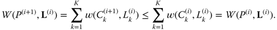
After this ![]() th iteration, we can now define at the next
th iteration, we can now define at the next ![]() th iteration a new representation
th iteration a new representation ![]() with
with ![]() and where we now have a better fit than we had before for the
and where we now have a better fit than we had before for the ![]() th iteration. This means that
th iteration. This means that ![]() ,
, ![]() . Hence,
. Hence,
Therefore, since ![]() decreases at each iteration, it must be converging. We note that a simple condition for the sequence
decreases at each iteration, it must be converging. We note that a simple condition for the sequence ![]() to be decreasing is that
to be decreasing is that ![]() for any partition
for any partition ![]() and any representation
and any representation ![]() . Thus, in the reallocation process, a reallocated individual which decreases the criteria the most will by definition be that individual which gives the best fit.
. Thus, in the reallocation process, a reallocated individual which decreases the criteria the most will by definition be that individual which gives the best fit.
As special cases, when ![]() is the mean of cluster
is the mean of cluster ![]() , we have the
, we have the ![]() ‐means algorithm, and when
‐means algorithm, and when ![]() is the medoid, we have the
is the medoid, we have the ![]() ‐medoid algorithm. Notice then that this implies that the
‐medoid algorithm. Notice then that this implies that the ![]() and
and ![]() of Eq. (6.1.5) correspond, respectively, to the
of Eq. (6.1.5) correspond, respectively, to the ![]() and
and ![]() of Eq. 5.2.1. Indeed, the representation of any cluster can be a density function (see Diday and Schroeder (1976)), a regression (see Charles (1977) and Liu (2016)), or more generally a canonical analysis (see Diday (1978, 1986a)), a factorial axis (see Diday (1972a,b)), a distance (see, e.g., Diday and Govaert (1977)), a functional curve (Diday and Simon (1976)), points of a population (Diday (1973)), and so on. For an overview, see Diday (1979), Diday and Simon (1976), and Diday (1989).
of Eq. 5.2.1. Indeed, the representation of any cluster can be a density function (see Diday and Schroeder (1976)), a regression (see Charles (1977) and Liu (2016)), or more generally a canonical analysis (see Diday (1978, 1986a)), a factorial axis (see Diday (1972a,b)), a distance (see, e.g., Diday and Govaert (1977)), a functional curve (Diday and Simon (1976)), points of a population (Diday (1973)), and so on. For an overview, see Diday (1979), Diday and Simon (1976), and Diday (1989).
Many names have been used for this general technique. For example, Diday (1971a,b, 1972b) refers to this as a “nuées dynamique” method, while in Diday (1973), Diday et al. (1974), and Diday and Simon (1976), it is called a “dynamic clusters” technique, and Jain and Dubes (1988) call it a “square error distortion” method. Bock (2007) calls it an “iterated minimum partition” method and Anderberg (1973) refers to it as a “nearest centroid sorting” method; these latter two descriptors essentially reflect the actual procedure as described in Chapter 6. This dynamical partitioning method can also be found in, e.g., Diday et al. (1974), Schroeder (1976), Scott and Symons (1971), Diday (1979), Celeux and Diebolt (1985), Celeux et al. (1989), Symons (1981), and Ralambondrainy (1995).
Another variant is the “self‐organizing maps” (SOM) method, or “Kohonen neural networks” method, described by Kohonen (2001). This method maps patterns onto a grid of units or neurons. In a comparison of the two methods, Bacão et al. (2005) concludes that the SOM method is less likely than the ![]() ‐means method to settle on local optima, but that the SOM method converges to the same result as that obtained by the
‐means method to settle on local optima, but that the SOM method converges to the same result as that obtained by the ![]() ‐means method . Hubert and Arabie (1985) compare some of these methods.
‐means method . Hubert and Arabie (1985) compare some of these methods.
While the ![]() ‐means method uses input coordinate values as its data, the
‐means method uses input coordinate values as its data, the ![]() ‐medoids method uses dissimilarities/distances as its input. This method is also known as the partitioning around mediods (PAM) method developed by Kaufman and Rousseeuw (1987) and Diday (1979). The algorithm works in the same way as does the
‐medoids method uses dissimilarities/distances as its input. This method is also known as the partitioning around mediods (PAM) method developed by Kaufman and Rousseeuw (1987) and Diday (1979). The algorithm works in the same way as does the ![]() ‐means algorithm but moves observations into clusters based on their dissimilarities/distances from cluster medoids (instead of cluster means). The medoids are representative but actual observations inside the cluster. Some variants use the median, midrange, or mode value as the medoid. Since the basic input elements are dissimilarities/distances, the method easily extends to symbolic data, where now dissimilarities/distances can be calculated using the results of Chapter 3s and . The PAM method is computationally intensive so is generally restricted to small data sets. Kaufman and Rousseeuw (1986) developed a version for large data sets called clustering large applications (CLARA). This version takes samples from the full data set, applies PAM to each sample, and then amalgamates the results.
‐means algorithm but moves observations into clusters based on their dissimilarities/distances from cluster medoids (instead of cluster means). The medoids are representative but actual observations inside the cluster. Some variants use the median, midrange, or mode value as the medoid. Since the basic input elements are dissimilarities/distances, the method easily extends to symbolic data, where now dissimilarities/distances can be calculated using the results of Chapter 3s and . The PAM method is computationally intensive so is generally restricted to small data sets. Kaufman and Rousseeuw (1986) developed a version for large data sets called clustering large applications (CLARA). This version takes samples from the full data set, applies PAM to each sample, and then amalgamates the results.
As a different approach, Goodall (1966) used a probabilistic similarity matrix to determine the reallocation step, while other researchers based this criterion on multivariate statistical analyses such as discriminant analysis. Another approach is to assume observations arise from a finite mixture of distributions, usually multivariate normal distributions. These model‐based methods require the estimation, often by maximum likelihood methods or Bayesian methods, of model parameters (mixture probabilities, and the distributional parameters such as means and variances) at each stage, before the partitioning process continues, as in, for example, the expectation‐maximization (EM) algorithm of Dempster et al. (1977). See, for example, McLachlan and Peel (2000), McLachlan and Basford (1988), Celeux and Diebolt (1985), Celeux and Govaert (1992, 1995), Celeux et al. (1989), and Banfield and Raftery (1993).
5.3 Hierarchies
In contrast to partitioning methods, hierarchical methods construct hierarchies which are nested clusters. Usually, these are depicted pictorially as trees or dendograms, thereby showing the relationships between the clusters, as in Figure 5.1. In this chapter, we make no distinction between monothetic methods (which focus on one variable at a time) or polythetic methods (which use all variables simultaneously) (see Chapter 7 , where the distinctions are made).
Note this definition of the hierarchy ![]() includes all the nodes of the tree. In contrast, the final clusters only, with none of the intermediate sub‐cluster/nodes, can be viewed as the bi‐partition
includes all the nodes of the tree. In contrast, the final clusters only, with none of the intermediate sub‐cluster/nodes, can be viewed as the bi‐partition ![]() (although the construction of a hierarchy
(although the construction of a hierarchy ![]() differs from that for a partition
differs from that for a partition ![]() ). Thus for a partition, the intersection of two clusters is empty (e.g., clusters
). Thus for a partition, the intersection of two clusters is empty (e.g., clusters ![]() and
and ![]() of Figure 5.1) whereas the intersection of two nested clusters in a hierarchy is not necessarily empty (e.g., clusters
of Figure 5.1) whereas the intersection of two nested clusters in a hierarchy is not necessarily empty (e.g., clusters ![]() and
and ![]() of Figure 5.1).
of Figure 5.1).
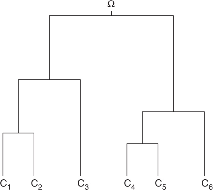
Figure 5.1 Clusters  as a partition at the end of a hierarchy.

Figure 5.2 Nodes‐clusters  of a hierarchy.
Hierarchical methodologies fall into two broad classes. Divisive clustering starts with the tree root ![]() containing all
containing all ![]() observations and divides this into two sub‐clusters
observations and divides this into two sub‐clusters ![]() and
and ![]() and so on, down to a final set of
and so on, down to a final set of ![]() clusters each with one observation. Thus, with reference to Figure 5.2, we start with one cluster
clusters each with one observation. Thus, with reference to Figure 5.2, we start with one cluster ![]() (containing
(containing ![]() observations) which is divided into
observations) which is divided into ![]() and
and ![]() , here each of three observations. Then, one of these (in this case
, here each of three observations. Then, one of these (in this case ![]() ) is further divided into, here,
) is further divided into, here, ![]() and
and ![]() . Then, cluster
. Then, cluster ![]() is divided into
is divided into ![]() and
and ![]() . The process continues until there are six clusters each containing just one observation.
. The process continues until there are six clusters each containing just one observation.
Agglomerative methods, on the other hand, start with ![]() clusters, with each observation being a one‐observation cluster at the bottom of the tree with successive merging of clusters upwards, until the final cluster consisting of all the observations (
clusters, with each observation being a one‐observation cluster at the bottom of the tree with successive merging of clusters upwards, until the final cluster consisting of all the observations (![]() ) is obtained. Thus, with reference to Figure 5.2, each of the six clusters
) is obtained. Thus, with reference to Figure 5.2, each of the six clusters ![]() contains one observation only. The two clusters
contains one observation only. The two clusters ![]() and
and ![]() are merged to form cluster
are merged to form cluster ![]() . Then,
. Then, ![]() and
and ![]() merge to form cluster
merge to form cluster ![]() . The next merging is when the clusters
. The next merging is when the clusters ![]() and
and ![]() merge to give
merge to give ![]() , or equivalently, at this stage (in two steps) the original single observation clusters
, or equivalently, at this stage (in two steps) the original single observation clusters ![]() ,
, ![]() , and
, and ![]() form the three‐observation cluster of
form the three‐observation cluster of ![]() . This process continues until all six observations in
. This process continues until all six observations in ![]() form the root node
form the root node ![]() .
.
Of course, for either of these methods, the construction can stop at some intermediate stage, such as between the formation of the clusters ![]() and
and ![]() in Figure 5.2 (indicated by the dotted line). In this case, the process stops with the four clusters
in Figure 5.2 (indicated by the dotted line). In this case, the process stops with the four clusters ![]() ,
, ![]() ,
, ![]() , and
, and ![]() . Indeed, such intermediate clusters may be more informative than might be a final complete tree with only one‐observation clusters as its bottom layer. Further, these interim clusters can serve as valuable input to the selection of initial clusters in a partitioning algorithm.
. Indeed, such intermediate clusters may be more informative than might be a final complete tree with only one‐observation clusters as its bottom layer. Further, these interim clusters can serve as valuable input to the selection of initial clusters in a partitioning algorithm.
At a given stage, how we decide which two clusters are to be merged in the agglomerative approach, or which cluster is to be bi‐partitioned, i.e., divided into two clusters in a divisive approach, is determined by the particular algorithm adopted by the researcher. There are many possible criteria used for this.
The motivating principle behind any hierarchical construction is to divide the data set ![]() into clusters which are internally as homogeneous as possible and externally as heterogeneous as possible. While some algorithms implicitly focus on maximizing the between‐cluster heterogeneities, and others focus on minimizing the within‐cluster homogeneities exclusively, most aim to balance both the between‐cluster variations and within‐cluster variations.
into clusters which are internally as homogeneous as possible and externally as heterogeneous as possible. While some algorithms implicitly focus on maximizing the between‐cluster heterogeneities, and others focus on minimizing the within‐cluster homogeneities exclusively, most aim to balance both the between‐cluster variations and within‐cluster variations.
Thus, divisive methods search to find the best bi‐partition at each stage, usually using a sum of squares approach which minimizes the total error sum of squares (in a classical setting) or a total within‐cluster variation (in a symbolic setting). More specifically, the cluster ![]() with
with ![]() observations has a total within‐cluster variation of
observations has a total within‐cluster variation of ![]() (say), described in Chapter 7 (Definition 7.1, Eq. (7.1.2)), and we want to divide the
(say), described in Chapter 7 (Definition 7.1, Eq. (7.1.2)), and we want to divide the ![]() observations into two disjoint sub‐clusters
observations into two disjoint sub‐clusters ![]() and
and ![]() so that the total within‐cluster variations of both
so that the total within‐cluster variations of both ![]() and
and ![]() satisfy
satisfy ![]() . How this is achieved varies with the different algorithms, but all seek to find that division which minimizes
. How this is achieved varies with the different algorithms, but all seek to find that division which minimizes ![]() . However, since these entities are functions of the distances (or dis/similarities) between observations in a cluster, different dissimilarities/distance functions will also produce differing hierarchies in general (though some naturally will be comparable for different dissimilarities/distance functions and/or different algorithms) (see Chapters 3 and ).
. However, since these entities are functions of the distances (or dis/similarities) between observations in a cluster, different dissimilarities/distance functions will also produce differing hierarchies in general (though some naturally will be comparable for different dissimilarities/distance functions and/or different algorithms) (see Chapters 3 and ).
In contrast, agglomerative methods seek to find the best merging of two clusters at each stage. How “best” is defined varies by the method, but typically involves a concept of merging the two “closest” observations. Most involve a dis/similarity (or distance) measure in some format. These include the following:
- Single‐link (or “nearest neighbor”) methods, where two clusters
 and
and  are merged if the dissimilarity between them is the minimum of all such dissimilarities across all pairs
  and
and  ,
,  . Thus, with reference to Figure 5.2, at the first step, since each cluster corresponds to a single observation
  , this method finds those two observations for which the dissimilarity/distance measure,
  , is minimized; here
  and
and  form
form  . At the next step, the process continues by finding the two clusters which have the minimum dissimilarity/distance between them. See Sneath and Sokal (1973).
 - Complete‐link (or “farthest neighbor”) methods are comparable to single‐link methods except that it is the maximum dissimilarity/distance at each stage that determines the best merger, instead of the minimum dissimilarity/distance. See Sneath and Sokal (1973).
- Ward's (or “minimum variance”) methods, where two clusters, of the set of clusters, are merged if they have the smallest squared Euclidean distance between their cluster centroids. This is proportional to a minimum increase in the error sum of squares for the newly merged cluster (across all potential mergers). See Ward (1963).
- There are several others, including average‐link (weighted average and group average), median‐link, flexible, centroid‐link, and so on. See, e.g, Anderberg (1973), Jain and Dubes (1988), McQuitty (1967), Gower (1971), Sokal and Michener (1958), Sokal and Sneath (1963), MacNaughton‐Smith et al. (1964), Lance and Williams (1967b) and Gordon (1987, 1999).
Clearly, as for divisive methods, these methods involve dissimilarity (or distance) functions in some form. A nice feature of the single‐link and complete‐link methods is that they are invariant to monotonic transformations of the dissimilarity matrices. The medium‐link method also retains this invariance property; however, it has a problem in implementation in that ties can frequently occur. The average‐link method loses this invariance property. The Ward criterion can retard the growth of large clusters, with outlier points tending to be merged at earlier stages of the clustering process. When the dissimilarity matrices are ultrametric (see Definition 3.4), single‐link and complete‐link methods produce the same tree. Furthermore, an ultrametric dissimilarity matrix will always allow a hierarchy tree to be built. Those methods based on Euclidean distances are invariant to orthogonal rotation of the variable axes.
In general, ties are a problem, and so usually algorithms assume no ties exist. However, ties can be broken by adding an arbitrarily small value ![]() to one distance; Jardine and Sibson (1971) show that, for the single‐link method, the results merge to the same tree as this perturbation
to one distance; Jardine and Sibson (1971) show that, for the single‐link method, the results merge to the same tree as this perturbation ![]() . Also, reversals can occur for median and centroid constructions, though they can be prevented when the distance between two clusters exceeds the maximum tree height for each separate cluster (see, e.g., Gordon (1987)).
. Also, reversals can occur for median and centroid constructions, though they can be prevented when the distance between two clusters exceeds the maximum tree height for each separate cluster (see, e.g., Gordon (1987)).
Gordon (1999), Punj and Stewart (1983), Jain and Dubes (1988), Anderberg (1973), Cormack (1971), Kaufman and Rousseeuw (1990), and Jain et al. (1999), among many other sources, provide an excellent coverage and comparative review of these methods, for both divisive and agglomerative approaches. While not all such comparisons are in agreement, by and large complete‐link methods are preferable to single‐link methods, though complete‐link methods have more problems with ties. The real agreement between these studies is that there is no one best dissimilarity/distance measure, no one best method, and no one best algorithm, though Kaufman and Rousseeuw (1990) argue strenuously that the group average‐link method is preferable. It all depends on the data at hand and the purpose behind the construction itself. For example, suppose in a map of roads it is required to find a road system, then a single‐link would likely be wanted, whereas if it is a region where types of housing clusters are sought, then a complete‐link method would be better. Jain et al. (1999) suggest that complete‐link methods are more useful than single‐link methods for many applications. In statistical applications, minimum variance methods tend to be used, while in pattern recognition, single‐link methods are more often used. Also, a hierarchy is in one‐to‐one correspondence with an ultrametric dissimilarity matrix (Johnson, 1967).
A pyramid is a type of agglomerative construction where now clusters can overlap. In particular, any given object can appear in two overlapping clusters. However, that object cannot appear in three or more clusters. This implies there is a linear order of the set of objects in ![]() . To construct a pyramid, the dissimilarity matrix must be a Robinson matrix (see Definition 3.6). Whereas a partition consists of non‐overlapping/disjoint clusters and a hierarchy consists of nested non‐overlapping clusters, a pyramid consists of nested overlapping clusters. Diday (1984, 1986b) introduces the basic principles, with an extension to spatial pyramids in Diday (2008). They are constructed from dissimilarity matrices by Diday (1986b), Diday and Bertrand (1986), and Gaul and Schader (1994).
. To construct a pyramid, the dissimilarity matrix must be a Robinson matrix (see Definition 3.6). Whereas a partition consists of non‐overlapping/disjoint clusters and a hierarchy consists of nested non‐overlapping clusters, a pyramid consists of nested overlapping clusters. Diday (1984, 1986b) introduces the basic principles, with an extension to spatial pyramids in Diday (2008). They are constructed from dissimilarity matrices by Diday (1986b), Diday and Bertrand (1986), and Gaul and Schader (1994).
For most methods, it is not possible to be assured that the resulting tree is globally optimal, only that it is step‐wise optimal. Recall that at each step/stage of the construction, an optimal criterion is being used; this does not necessarily guarantee optimally for the complete tree. Also, while step‐wise optimality pertains, once that stage is completed (be this up or down the tree, i.e., divisive or agglomerative clustering), there is no allowance to go back to any earlier stage.
There are many different formats for displaying a hierarchy tree; Figure 5.1 is but one illustration. Gordon (1999) provides many representations. For each representation, there are ![]() different orders of the tree branches of the same hierarchy of
different orders of the tree branches of the same hierarchy of ![]() objects. Thus, for example, a hierarchy on the three objects
objects. Thus, for example, a hierarchy on the three objects ![]() can take any of the
can take any of the ![]() forms shown in Figure 5.3. However, a tree with the object 3 as a branch in‐between the branches 1 and 2 is not possible. In contrast, there are only two possible orderings if a pyramid is built on these three objects, namely,
forms shown in Figure 5.3. However, a tree with the object 3 as a branch in‐between the branches 1 and 2 is not possible. In contrast, there are only two possible orderings if a pyramid is built on these three objects, namely, ![]() and
and ![]() .
.

Figure 5.3 Different orders for a hierarchy of objects  .
.
A different format is a so‐called dendogram, which is a hierarchy tree on which a measure of “height” has been added at each stage of the tree's construction.
It is easy to show that (Gordon, 1999), for any two observations in ![]() with realizations
with realizations ![]() ,
, ![]() , the height satisfies the ultrametric property, i.e.,
, the height satisfies the ultrametric property, i.e.,
One such measure is ![]() where
where ![]() is the explained rate (i.e., the proportion of total variation in
is the explained rate (i.e., the proportion of total variation in ![]() explained by the tree) at stage
explained by the tree) at stage ![]() of its construction (see section 7.4 for details).
of its construction (see section 7.4 for details).
There are many divisive and agglomerative algorithms in the literature for classical data, but few have been specifically designed for symbolic‐valued observations. However, those (classical) algorithms based on dissimilarities/distances can sometimes be extended to symbolic data where now the symbolic dissimilarities/distances between observations are utilized. Some such extensions are covered in Chapters 7 and 8.
5.4 Illustration
We illustrate some of the clustering methods outlined in this chapter. The first three provide many different analyses on the same data set, showing how different methods can give quite different results. The fourth example shows how symbolic analyses utilizing internal variations are able to identify clusters that might be missed when using a classical analysis on the same data.
5.5 Other Issues
The choice of an appropriate number of clusters is still unsolved for partitioning and hierarchical procedures. In the context of classical data, several researchers have tried to provide answers, e.g., Milligan and Cooper (1985), and Tibshirani and Walther (2005). One approach is to run the algorithm for several specific values of ![]() and then to compare the resulting approximate weight of evidence (AWE) suggested by Banfield and Raftery (1993) for hierarchies and Fraley and Raftery (1998) for mixture distribution model‐based partitions. Kim and Billard (2011) extended the Dunn (1974) and Davis and Bouldin (1979) indices to develop quality indices in the hierarchical clustering context for histogram observations which can be used to identify a “best” value for
and then to compare the resulting approximate weight of evidence (AWE) suggested by Banfield and Raftery (1993) for hierarchies and Fraley and Raftery (1998) for mixture distribution model‐based partitions. Kim and Billard (2011) extended the Dunn (1974) and Davis and Bouldin (1979) indices to develop quality indices in the hierarchical clustering context for histogram observations which can be used to identify a “best” value for ![]() (see section 7.4).
(see section 7.4).
Questions around robustness and validation of obtained clusters are largely unanswered. Dubes and Jain (1979), Milligan and Cooper (1985), and Punj and Stewart (1983) provide some insights for classical data. Fräti et al. (2014) and Lisboa et al. (2013) consider these questions for the ![]() ‐means approach to partitions. Hardy (2007) and Hardy and Baume (2007) consider the issue with respect to hierarchies for interval‐valued observations.
‐means approach to partitions. Hardy (2007) and Hardy and Baume (2007) consider the issue with respect to hierarchies for interval‐valued observations.
Other topics not yet developed for symbolic data include, e.g., block modeling (see, e.g., Doreian et al. (2005) and Batagelj and Ferligoj (2000)), constrained or relational clustering where internal connectedness (such as geographical boundaries) is imposed (e.g., Ferligoj and Batagelj (1982, 1983, 1992)), rules‐based algorithms along the lines developed by Reynolds et al. (2006) for classical data, and analyses for large temporal and spatial networks explored by Batagelj et al. (2014).
In a different direction, decision‐based trees have been developed by a number of researchers, such as the classification and regression trees (CART) of Breiman et al. (1984) for classical data, in which a dependent variable is a function of predictor variables as in standard regression analysis. Limam (2005), Limam et al. (2004), Winsberg et al. (2006), Seck (2012), and Seck et al. (2010), have considered CART methods for symbolic data, but much more remains to be done.
In a nice review of model‐based clustering for classical data, Fraley and Raftery (1998) introduce a partitioning approach by combining hierarchical clustering with the expectation‐maximization algorithm of Dempster et al. (1977). A stochastic expectation‐maximization algorithm was developed in Celeux and Diebolt (1985), a classification expectation‐maximization algorithm was introduced by Celeux and Govaert (1992), and a Monte Carlo expectation‐maximization algorithm was described by Wei and Tanner (1990). How these might be adapted to a symbolic‐valued data setting are left as open problems.
Other exploratory methods include factor analysis and principal component analysis, both based on eigenvalues/eigenvectors of the correlation matrices, or projection pursuit (e.g. Friedman, 1987). Just as different distance measures can produce different hierarchies, so can the different approaches (clustering per se compared to eigenvector‐based methods) produce differing patterns. For example, in Chapter 7 , Figure 7.6 shows the hierarchy that emerged when a monothethic divisive clustering approach (see section 7.2 , Example 7.7) was applied to the temperature data set of Table 7.9. The resultant clusters are different from those obtained in Billard and Le‐Rademacher (2012) when a principal component analysis was applied to those same data (see Figure 5.14).

Figure 5.14 Principal component analysis on China temperature data of Table 7.9.