
2
Symbolic Data: Basics
In this chapter, we describe what symbolic data are, how they may arise, and their different formulations. Some data are naturally symbolic in format, while others arise as a result of aggregating much larger data sets according to some scientific question(s) that generated the data sets in the first place. Thus, section 2.2.1 describes non‐modal multi‐valued or lists of categorical data, with modal multi‐valued data in section 2.2.2; lists or multi‐valued data can also be called simply categorical data. Section 2.2.3 considers interval‐valued data, with modal interval data more commonly known as histogram‐valued data in section 2.2.4. We begin, in section 2.1, by considering the distinctions and similarities between individuals, classes, and observations. How the data arise, such as by aggregation, is discussed in section 2.3. Basic descriptive statistics are presented in section 2.4. Except when necessary for clarification purposes, we will write “interval‐valued data” as “interval data” for simplicity; likewise, for the other types of symbolic data.
It is important to remember that symbolic data, like classical data, are just different manifestations of sub‐spaces of the ![]() ‐dimensional space
‐dimensional space ![]() always dealing with the same random variables. A classical datum is a point in
always dealing with the same random variables. A classical datum is a point in ![]() , whereas a symbolic value is a hypercube or a Cartesian product of distributions in
, whereas a symbolic value is a hypercube or a Cartesian product of distributions in ![]() . Thus, for example, the
. Thus, for example, the ![]() ‐dimensional random variable
‐dimensional random variable ![]() measuring height and weight (say) can take a classical value
measuring height and weight (say) can take a classical value ![]() inches and
inches and ![]() kg, or it may take a symbolic value with
kg, or it may take a symbolic value with ![]() and
and ![]() interval values which form a rectangle or a hypercube in the plane. That is, the random variable is itself unchanged, but the realizations of that random variable differ depending on the format. However, it is also important to recognize that since classical values are special cases of symbolic values, then regardless of analytical technique, classical analyses and symbolic analyses should produce the same results when applied to those classical values.
interval values which form a rectangle or a hypercube in the plane. That is, the random variable is itself unchanged, but the realizations of that random variable differ depending on the format. However, it is also important to recognize that since classical values are special cases of symbolic values, then regardless of analytical technique, classical analyses and symbolic analyses should produce the same results when applied to those classical values.
2.1 Individuals, Classes, Observations, and Descriptions
In classical statistics, we talk about having a random sample of ![]() observations
observations ![]() as outcomes for a random variable
as outcomes for a random variable ![]() . More precisely, we say
. More precisely, we say ![]() is the observed value for individual
is the observed value for individual ![]() ,
, ![]() . A particular observed value may be
. A particular observed value may be ![]() , say. We could equivalently say the description of the
, say. We could equivalently say the description of the ![]() th individual is
th individual is ![]() . Usually, we think of an individual as just that, a single individual. For example, our data set of
. Usually, we think of an individual as just that, a single individual. For example, our data set of ![]() individuals may record the height
individuals may record the height ![]() of individuals, Bryson, Grayson, Ethan, Coco, Winston, Daisy, and so on. The “individual” could also be an inanimate object such as a particular car model with
of individuals, Bryson, Grayson, Ethan, Coco, Winston, Daisy, and so on. The “individual” could also be an inanimate object such as a particular car model with ![]() describing its capacity, or some other measure relating to cars. On the other hand, the “individual” may represent a class of individuals. For example, the data set consisting of
describing its capacity, or some other measure relating to cars. On the other hand, the “individual” may represent a class of individuals. For example, the data set consisting of ![]() individuals may be
individuals may be ![]() classes of car models, Ford, Renault, Honda, Volkswagen, Nova, Volvo, … , with
classes of car models, Ford, Renault, Honda, Volkswagen, Nova, Volvo, … , with ![]() recording the car's speed over a prescribed course, etc. However individuals may be defined, the realization of
recording the car's speed over a prescribed course, etc. However individuals may be defined, the realization of ![]() for that individual is a single point value from its domain
for that individual is a single point value from its domain ![]() .
.
If the random variable ![]() takes quantitative values, then the domain (also called the range or observation space) is
takes quantitative values, then the domain (also called the range or observation space) is ![]() taking values on the real line
taking values on the real line ![]() , or a subset of
, or a subset of ![]() such as
such as ![]() if
if ![]() can only take non‐negative or zero values. When
can only take non‐negative or zero values. When ![]() takes qualitative values, then a classically valued observation takes one of two possible values such as
takes qualitative values, then a classically valued observation takes one of two possible values such as ![]() Yes, No
Yes, No![]() or coded to
or coded to ![]() , for example. Typically, if there are several categories of possible values, e.g., bird colors with domain
, for example. Typically, if there are several categories of possible values, e.g., bird colors with domain ![]() , a classical analysis will include a different random variable for each category and then record the presence (Yes) or absence (No) of each category. When there are
, a classical analysis will include a different random variable for each category and then record the presence (Yes) or absence (No) of each category. When there are ![]() random variables, then the domain of
random variables, then the domain of ![]() is
is ![]() .
.
In contrast, when the data are symbolic‐valued, the observations ![]() are typically realizations that emerge after aggregating observed values for the random variable
are typically realizations that emerge after aggregating observed values for the random variable ![]() across some specified class or category of interest (see section 2.3). Thus, for example, observations may refer now to
across some specified class or category of interest (see section 2.3). Thus, for example, observations may refer now to ![]() classes, or categories, of age
classes, or categories, of age![]() income, or to
income, or to ![]() species of dogs, and so on. Thus, the class Boston (say) has a June temperature range of
species of dogs, and so on. Thus, the class Boston (say) has a June temperature range of ![]() F,
F, ![]() F]. In the language of symbolic analysis, the individuals are ground‐level or order‐one individuals and the aggregations – classes – are order‐two individuals or “objects” (see, e.g., Diday (1987, 2016), Bock and Diday (2000a,b), Billard and Diday (2006a), or Diday and Noirhomme‐Fraiture (2008)).
F]. In the language of symbolic analysis, the individuals are ground‐level or order‐one individuals and the aggregations – classes – are order‐two individuals or “objects” (see, e.g., Diday (1987, 2016), Bock and Diday (2000a,b), Billard and Diday (2006a), or Diday and Noirhomme‐Fraiture (2008)).
On the other hand, suppose Gracie's pulse rate ![]() is the interval
is the interval ![]() . Gracie is a single individual and a classical value for her pulse rate might be
. Gracie is a single individual and a classical value for her pulse rate might be ![]() . However, this interval of values would result from the collection, or aggregation, of Gracie's classical pulse rate values over some specified time period. In the language of symbolic data, this interval represents the pulse rate of the class “Gracie”. However, this interval may be the result of aggregating the classical point values of all individuals named “Gracie” in some larger data base. That is, some symbolic realizations may relate to one single individual, e.g., Gracie, whose pulse rate may be measured as
. However, this interval of values would result from the collection, or aggregation, of Gracie's classical pulse rate values over some specified time period. In the language of symbolic data, this interval represents the pulse rate of the class “Gracie”. However, this interval may be the result of aggregating the classical point values of all individuals named “Gracie” in some larger data base. That is, some symbolic realizations may relate to one single individual, e.g., Gracie, whose pulse rate may be measured as ![]() over time, or to a set of all those Gracies of interest. The context should make it clear which situation prevails.
over time, or to a set of all those Gracies of interest. The context should make it clear which situation prevails.
In this book, symbolic realizations for the observation ![]() can refer interchangeably to the description
can refer interchangeably to the description ![]() of classes or categories or “individuals”
of classes or categories or “individuals” ![]() ,
, ![]() , that is, simply,
, that is, simply, ![]() will be the unit (which is itself a class, category, individual, or observation) that is described by
will be the unit (which is itself a class, category, individual, or observation) that is described by ![]() . Furthermore, in the language of symbolic data, the realization of
. Furthermore, in the language of symbolic data, the realization of ![]() is referred to as the “description”
is referred to as the “description” ![]() of
of ![]() ,
, ![]() . For simplicity, we write simply
. For simplicity, we write simply ![]() ,
, ![]() .
.
2.2 Types of Symbolic Data
2.2.1 Multi‐valued or Lists of Categorical Data
We have a random variable ![]() whose realization is the set of values
whose realization is the set of values ![]() from the set of possible values or categories
from the set of possible values or categories ![]() , where
, where ![]() and
and ![]() with
with ![]() are finite. Typically, for a symbolic realization,
are finite. Typically, for a symbolic realization, ![]() , whereas for a classical realization,
, whereas for a classical realization, ![]() . This realization is called a list (of
. This realization is called a list (of ![]() categories from
categories from ![]() ) or a multi‐valued realization, or even a multi‐categorical realization, of
) or a multi‐valued realization, or even a multi‐categorical realization, of ![]() . Formally, we have the following definition.
. Formally, we have the following definition.
Notice that, in general, the number of categories ![]() in the actual realization differs across realizations (i.e.,
in the actual realization differs across realizations (i.e., ![]() ),
), ![]() , and across variables
, and across variables ![]() (i.e.,
(i.e., ![]() ),
), ![]() .
.
Table 2.1 List or multi‐valued data: regional utilities (Example 2.1)
| Region |
Major utility | Cost |
| 1 | [190, 230] | |
| 2 | [21.5, 25.5] | |
| 3 | [40, 53] | |
| 4 | 15.5 | |
| 5 | [25, 30] | |
| 6 | 46.0 | |
| 7 | [37, 43] |
While list data mostly take qualitative values that are verbal descriptions of an outcome, such as the types of utility usages in Example 2.1, quantitative values such as coded values ![]() may be the recorded value. These are not necessarily the same as ordered categorical values such as
may be the recorded value. These are not necessarily the same as ordered categorical values such as ![]() =
= ![]() small, medium, large
small, medium, large![]() . Indeed, a feature of categorical values is that there is no prescribed ordering of the listed realizations. For example, for the seventh region (
. Indeed, a feature of categorical values is that there is no prescribed ordering of the listed realizations. For example, for the seventh region (![]() ) in Table 2.1, the description
) in Table 2.1, the description ![]() electricity, coal
electricity, coal![]() is exactly the same description as
is exactly the same description as ![]() coal, electricity
coal, electricity![]() , i.e., the same region. This feature does not carry over to quantitative values such as histograms (see section 2.2.4).
, i.e., the same region. This feature does not carry over to quantitative values such as histograms (see section 2.2.4).
2.2.2 Modal Multi‐valued Data
Modal lists or modal multi‐valued data (sometimes called modal categorical data) are just list or multi‐valued data but with each realized category occurring with some specified weight such as an associated probability. Examples of non‐probabilistic weights include the concepts of capacities, possibilities, and necessities (see Billard and Diday, 2006a, Chapter 2 ; see also Definitions 2.6–2.9 in section 2.2.5). In this section and throughout most of this book, it is assumed that the weights are probabilities; suitable adjustment for other weights is left to the reader.
Without loss of generality, we can write the number of categories from ![]() for the random variable
for the random variable ![]() , as
, as ![]() , for all
, for all ![]() , by simply giving unrealized categories (
, by simply giving unrealized categories (![]() , say) the probability
, say) the probability ![]() . Furthermore, the non‐modal multi‐valued realization of Eq. 2.2.1 can be written as a modal multi‐valued observation of Eq. 2.2.2 by assuming actual realized categories from
. Furthermore, the non‐modal multi‐valued realization of Eq. 2.2.1 can be written as a modal multi‐valued observation of Eq. 2.2.2 by assuming actual realized categories from ![]() occur with equal probability, i.e.,
occur with equal probability, i.e., ![]() for
for ![]() , and unrealized categories occur with probability zero, for each
, and unrealized categories occur with probability zero, for each ![]() .
.
Table 2.2 Modal multi‐valued data: smoking deaths (![]() ) (Example 2.2)
) (Example 2.2)
| Proportion |
|||
| Region |
Smoking | Lung cancer | Respiratory |
| 1 | 0.628 | 0.184 | 0.188 |
| 2 | 0.623 | 0.202 | 0.175 |
| 3 | 0.650 | 0.197 | 0.153 |
| 4 | 0.626 | 0.209 | 0.165 |
| 5 | 0.690 | 0.160 | 0.150 |
| 6 | 0.631 | 0.204 | 0.165 |
| 7 | 0.648 | ||
| 8 | 1.000 | ||
2.2.3 Interval Data
A classical realization for quantitative data takes a point value on the real line ![]() . An interval‐valued realization takes values from a subset of
. An interval‐valued realization takes values from a subset of ![]() . This is formally defined as follows.
. This is formally defined as follows.
There are numerous examples of naturally occurring symbolic data sets. One such scenario exists in the next example.
Table 2.3 Interval data: weather stations (Example 2.4)
| Station | |||
| 1 | [ |
[17.0, 26.5] | 4.82 |
| 2 | [ |
[12.9, 23.0] | 14.78 |
| 3 | [ |
[10.8, 23.2] | 73.16 |
| 4 | [10.0, 17.7] | [24.2, 33.8] | 2.38 |
| 5 | [11.5, 17.7] | [25.8, 33.5] | 1.44 |
| 6 | [11.8, 19.2] | [25.6, 32.6] | 0.02 |
2.2.4 Histogram Data
Histogram data usually result from the aggregation of several values of quantitative random variables into a number of sub‐intervals. More formally, we have the following definition.
Usually, histogram sub‐intervals are closed at the left end and open at the right end except for the last sub‐interval, which is closed at both ends. Furthermore, note that the number of histogram sub‐intervals ![]() differs across
differs across ![]() and across
and across ![]() . For the special case that
. For the special case that ![]() , and hence
, and hence ![]() for all
for all ![]() , the histogram is an interval.
, the histogram is an interval.
Table 2.4 Histogram data: flight times (Example 2.5)
| Airline | |
| 1 | |
| 2 | |
| 3 | |
| 4 | |
| 5 | |
| 6 | |
| 7 | |
| 8 | |
| 9 | |
| 10 |
In the context of symbolic data methodology, the starting data are already in a histogram format. All data, including histogram data, can themselves be aggregated to form histograms (see section 2.4.4).
2.2.5 Other Types of Symbolic Data
A so‐called mixed data set is one in which not all of the ![]() variables take the same format. Instead, some may be interval data, some histograms, some lists, etc.
variables take the same format. Instead, some may be interval data, some histograms, some lists, etc.
Table 2.5 Mixed‐valued data: joggers (Example 2.6)
| Group |
||
| 1 | [73, 114] | {[5.3, 6.2), 0.3; [6.2, 7.1), 0.5; [7.1, 8.3], 0.2} |
| 2 | [70, 100] | {[5.5, 6.9), 0.4; [6.7, 8.0), 0.4; [8.0, 9.0], 0.2} |
| 3 | [69, 91] | {[5.1, 6.6), 0.4; [6.6, 7.4), 0.4; [7.4, 7.8], 0.2} |
| 4 | [59, 89] | {[3.7, 5.8), 0.6; [5.8, 6.3], 0.4} |
| 5 | [61, 87] | {[4.5, 5.9), 0.4; [5.9, 6.2], 0.6} |
| 6 | [69, 95] | {[4.1, 6.1), 0.5; [6.1, 6.9], 0.5} |
| 7 | [65, 78] | {[2.4, 4.8), 0.3; [4.8, 5.7), 0.5; [5.7, 6.2], 0.2} |
| 8 | [58, 83] | {[2.1, 5.4), 0.2; [5.4, 6.0), 0.5; [6.0, 6.9], 0.3} |
| 9 | [79, 103] | {[4.8, 6.5), 0.3; [6.5, 7.4); 0.5; [7.4, 8.2], 0.2} |
| 10 | [40, 60] | {[3.2, 4.1), 0.6; [4.1, 6.7], 0.4} |
Other types of symbolic data include probability density functions or cumulative distributions, as in the observations in Table 2.6(a), or models such as the time series models for the observations in Table 2.6(b).
Table 2.6 Some other types of symbolic data
| Description of |
||
| (a) | 1 | Distributed as a normal |
| 2 | Distributed as a normal |
|
| 3 | Distributed as exponential ( |
|
| (b) | 5 | Follows an AR(1) time‐series model |
| 6 | Follows a MA |
|
| 7 | Is a first‐order Markov chain | |
The modal multi‐valued data of section 2.2.2 and the histogram data of section 2.2.4 use probabilities as the weights of the categories and the histogram sub‐intervals; see Eqs. 2.2.2 and 2.2.4, respectively. While these weights are the most common seen by statistical analysts, there are other possible weights. First, let us define a more general weighted modal type of observation. We take the number of variables to be ![]() ; generalization to
; generalization to ![]() follows readily.
follows readily.
Thus, for a modal list or multi‐valued observation of Definition 2.2, the category ![]() and the probability
and the probability ![]() . Likewise, for a histogram observation of Definition 2.4, the sub‐interval
. Likewise, for a histogram observation of Definition 2.4, the sub‐interval ![]() occurs with relative frequency
occurs with relative frequency ![]() , which corresponds to the weight
, which corresponds to the weight ![]() ,
, ![]() . Note, however, that in Definition 2.5 the condition
. Note, however, that in Definition 2.5 the condition ![]() does not necessarily hold, unlike pure modal multi‐valued and histogram observations (see Eqs. 2.2.2 and 2.2.4, respectively). Thus, in these two cases, the weights
does not necessarily hold, unlike pure modal multi‐valued and histogram observations (see Eqs. 2.2.2 and 2.2.4, respectively). Thus, in these two cases, the weights ![]() are probabilities or relative frequencies. The following definitions relate to situations when the weights do not necessarily sum to one. As before,
are probabilities or relative frequencies. The following definitions relate to situations when the weights do not necessarily sum to one. As before, ![]() can differ from observation to observation.
can differ from observation to observation.
More examples for these cases can be found in Diday (1995) and Billard and Diday (2006a). This book will restrict attention to modal list or multi‐valued data and histogram data cases. However, many of the methodologies in the remainder of the book apply equally to any weights ![]() , including those for capacities, credibilities, possibilities, and necessities.
, including those for capacities, credibilities, possibilities, and necessities.
More theoretical aspects of symbolic data and concepts along with some philosophical aspects can be found in Billard and Diday (2006a, Chapter 2 ).
2.3 How do Symbolic Data Arise?
Symbolic data arise in a myriad of ways. One frequent source results when aggregating larger data sets according to some criteria, with the criteria usually driven by specific operational or scientific questions of interest.
For example, a medical data set may consist of millions of observations recording a slew of medical information for each individual for every visit to a healthcare facility since the year 1990 (say). There would be records of demographic variables (such as age, gender, weight, height, ![]() ), geographical information (such as street, city, county, state, country of residence, etc.), basic medical tests results (such as pulse rate, blood pressure, cholesterol level, glucose, hemoglobin, hematocrit,
), geographical information (such as street, city, county, state, country of residence, etc.), basic medical tests results (such as pulse rate, blood pressure, cholesterol level, glucose, hemoglobin, hematocrit, ![]() ), specific aliments (such as whether or not the patient has diabetes, a heart condition and if so what, i.e. mitral value syndrome, congestive heart failure, arrhythmia, diverticulitis, myelitis, etc.). There would be information as to whether the patient had a heart attack (and the prognosis) or cancer symptoms (such as lung cancer, lymphoma, brain tumor, etc.). For given aliments, data would be recorded indicating when and what levels of treatments were applied and how often, and so on. The list of possible symptoms is endless. The pieces of information would in analytic terms be the variables (for which the number
), specific aliments (such as whether or not the patient has diabetes, a heart condition and if so what, i.e. mitral value syndrome, congestive heart failure, arrhythmia, diverticulitis, myelitis, etc.). There would be information as to whether the patient had a heart attack (and the prognosis) or cancer symptoms (such as lung cancer, lymphoma, brain tumor, etc.). For given aliments, data would be recorded indicating when and what levels of treatments were applied and how often, and so on. The list of possible symptoms is endless. The pieces of information would in analytic terms be the variables (for which the number ![]() is also large), while the information for each individual for each visit to the healthcare facility would be an observation (where the number of observations
is also large), while the information for each individual for each visit to the healthcare facility would be an observation (where the number of observations ![]() in the data set can be extremely large). Trying to analyze this data set by traditional classical methods is likely to be too difficult to manage.
in the data set can be extremely large). Trying to analyze this data set by traditional classical methods is likely to be too difficult to manage.
It is unlikely that the user of this data set, whether s/he be a medical insurer or researcher or maybe even the patient him/herself, is particularly interested in the data for a particular visit to the care provider on some specific date. Rather, interest would more likely center on a particular disease (angina, say), or respiratory diseases in a particular location (Lagos, say), and so on. Or, the focus may be on age ![]() gender classes of patients, such as 26‐year‐old men or 35‐year‐old women, or maybe children (aged 17 years and under) with leukemia, again the list is endless. In other words, the interest is on characteristics between different groups of individuals (also called classes or categories, but these categories should not be confused with the categories that make up the lists or multi‐valued types of data of sections 2.2.1 and 2.2.2).
gender classes of patients, such as 26‐year‐old men or 35‐year‐old women, or maybe children (aged 17 years and under) with leukemia, again the list is endless. In other words, the interest is on characteristics between different groups of individuals (also called classes or categories, but these categories should not be confused with the categories that make up the lists or multi‐valued types of data of sections 2.2.1 and 2.2.2).
However, when the researcher looks at the accumulated data for a specific group, 50‐year‐old men with angina living in the New England district (say), it is unlikely all such individuals weigh the same (or have the same pulse rate, or the same blood pressure measurement, etc.). Rather, thyroid measurements may take values along the lines of, e.g., ![]() . These values could be aggregated into an interval to give
. These values could be aggregated into an interval to give ![]() or they could be aggregated as a histogram realization (especially if there are many values being aggregated). In general, aggregating all the observations which satisfy a given group/class/category will perforce give realizations that are symbolic valued. In other words, these aggregations produce the so‐called second‐level observations of Diday (1987). As we shall see in section 2.4, taking the average of these values for use in a (necessarily) classical methodology will give an answer certainly, but also most likely that answer will not be correct.
or they could be aggregated as a histogram realization (especially if there are many values being aggregated). In general, aggregating all the observations which satisfy a given group/class/category will perforce give realizations that are symbolic valued. In other words, these aggregations produce the so‐called second‐level observations of Diday (1987). As we shall see in section 2.4, taking the average of these values for use in a (necessarily) classical methodology will give an answer certainly, but also most likely that answer will not be correct.
Instead of a medical insurer's database, an automobile insurer would aggregate various entities (such as pay‐outs) depending on specific classes, e.g., age ![]() gender of drivers or type of car (Volvo, Renault, Chevrolet,
gender of drivers or type of car (Volvo, Renault, Chevrolet, ![]() ), including car type by age and gender, or maybe categories of drivers (such as drivers of red convertibles). Statistical agencies publish their census results according to groups or categories of households. For example, salary data are published as ranges such as
), including car type by age and gender, or maybe categories of drivers (such as drivers of red convertibles). Statistical agencies publish their census results according to groups or categories of households. For example, salary data are published as ranges such as ![]() –
–![]() , i.e., the interval
, i.e., the interval ![]() in 1000s of $.
in 1000s of $.
Let us illustrate this approach more concretely through the following example.
Most symbolic data sets will arise from these types of aggregations usually of large data sets but it can be aggregation of smaller data sets. A different situation can arise from some particular scientific question, regardless of the size of the data set. We illustrate this via a question regarding hospitalizations of cardiac patients, described more fully in Quantin et al. (2011).
There are numerous other situations which perforce are described by symbolic data. Species data are examples of naturally occurring symbolic data. Data with minimum and maximum values, such as the temperature data of Table 2.4, also occur as a somewhat natural way to record measurements of interest. Many stockmarket values are reported as high and low values daily (or weekly, monthly, annually). Pulse rates may more accurately be recorded as ![]() , i.e.,
, i.e., ![]() rather than the midpoint value of 64; blood pressure values are notorious for “bouncing around”, so that a given value of say 73 for diastolic blood pressure may more accurately be
rather than the midpoint value of 64; blood pressure values are notorious for “bouncing around”, so that a given value of say 73 for diastolic blood pressure may more accurately be ![]() . Sensitive census data, such as age, may be given as
. Sensitive census data, such as age, may be given as ![]() , and so on. There are countless examples.
, and so on. There are countless examples.
A question that can arise after aggregation has occurred deals with the handling of outlier values. For example, suppose data aggregated into intervals produced an interval with specific values ![]() . Or, better yet, suppose there were many many observations between 25 and 30 along with the single value 9. In mathematical terms, our interval, after aggregation, can be formally written as [a,b], where
. Or, better yet, suppose there were many many observations between 25 and 30 along with the single value 9. In mathematical terms, our interval, after aggregation, can be formally written as [a,b], where
where ![]() is the set of all
is the set of all ![]() values aggregated into the interval
values aggregated into the interval ![]() . In this case, we obtain the interval
. In this case, we obtain the interval ![]() . However, intuitively, we conclude that the value 9 is an outlier and really does not belong to the aggregations in the interval
. However, intuitively, we conclude that the value 9 is an outlier and really does not belong to the aggregations in the interval ![]() . Suppose instead of the value 9, we had a value 21, which, from Eq. 2.3.1, gives the interval
. Suppose instead of the value 9, we had a value 21, which, from Eq. 2.3.1, gives the interval ![]() . Now, it may not be at all clear if the value 21 is an outlier or if it truly belongs to the interval of aggregated values. Since most analyses involving interval data assume that observations within an interval are uniformly spread across that interval, the question becomes one of testing for uniformity across those intervals. Stéphan (1998), Stéphan et al. (2000), and Cariou and Billard (2015) have developed tests of uniformity, gap tests and distance tests, to help address this issue. They also give some reduction algorithms to achieve the deletion of genuine outliers.
. Now, it may not be at all clear if the value 21 is an outlier or if it truly belongs to the interval of aggregated values. Since most analyses involving interval data assume that observations within an interval are uniformly spread across that interval, the question becomes one of testing for uniformity across those intervals. Stéphan (1998), Stéphan et al. (2000), and Cariou and Billard (2015) have developed tests of uniformity, gap tests and distance tests, to help address this issue. They also give some reduction algorithms to achieve the deletion of genuine outliers.
2.4 Descriptive Statistics
In this section, basic descriptive statistics, such as sample means, sample variances and covariances, and histograms, for the differing types of symbolic data are briefly described. For quantitative data, these definitions implicitly assume that within each interval, or sub‐interval for histogram observations, observations are uniformly spread across that interval. Expressions for the sample mean and sample variance for interval data were first derived by Bertrand and Goupil (2000). Adjustments for non‐uniformity can be made. For list multi‐valued data, the sample mean and sample variance given herein are simply the respective classical values for the probabilities associated with each of the corresponding categories in the variable domain.
2.4.1 Sample Means
2.4.2 Sample Variances
Let us consider Eq. 2.4.5 more carefully. For these observations, it can be shown that the total sum of squares (SS), Total SS, i.e., ![]() , can be written as
, can be written as

where ![]() is the overall mean of Eq. 2.4.2, and where the sample mean of the observation
is the overall mean of Eq. 2.4.2, and where the sample mean of the observation ![]() is
is
The term inside the second summation in Eq. 2.4.6 equals ![]() given in Eq. 2.4.5 when
given in Eq. 2.4.5 when ![]() . That is, this is a measure of the internal variation, the internal variance, of the single observation
. That is, this is a measure of the internal variation, the internal variance, of the single observation ![]() . When summed over all such observations,
. When summed over all such observations, ![]() , we obtain the internal variation of all
, we obtain the internal variation of all ![]() observations; we call this the Within SS. To illustrate, suppose we have a single observation
observations; we call this the Within SS. To illustrate, suppose we have a single observation ![]() . Then, substituting into Eq. 2.4.5, we obtain the sample variance as
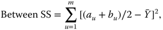
. Then, substituting into Eq. 2.4.5, we obtain the sample variance as ![]() , i.e., interval observations each contain internal variation. The first term in Eq. 2.4.6 is the variation of the interval midpoints across all observations, i.e., the Between SS.
, i.e., interval observations each contain internal variation. The first term in Eq. 2.4.6 is the variation of the interval midpoints across all observations, i.e., the Between SS.
Hence, we can write
where

By assuming that values across an interval are uniformly spread across the interval, we see that the Within SS can also be obtained from

Therefore, researchers, who upon aggregation of sets of classical data restrict their analyses to the average of the symbolic observation (such as interval means) are discarding important information; they are ignoring the internal variations (i.e., the Within SS) inherent to their data.
When the data are classically valued, with ![]() , then
, then ![]() and hence the Within SS of Eq. 2.4.10 is zero and the Between SS of Eq. 2.4.9 is the same as the Total SS for classical data. Hence, the sample variance of Eq. 2.4.5 for interval data reduces to its classical counterpart for classical point data, as it should.
and hence the Within SS of Eq. 2.4.10 is zero and the Between SS of Eq. 2.4.9 is the same as the Total SS for classical data. Hence, the sample variance of Eq. 2.4.5 for interval data reduces to its classical counterpart for classical point data, as it should.
As for intervals, we can show that the total variation for histogram data consists of two parts, as in Eq. 2.4.8, where now its components are given, respectively, by
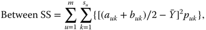
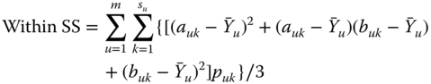
with

It is readily seen that for the special case of interval data, where now ![]() and hence
and hence ![]() for all
for all ![]() , the histogram sample variance of Eq. 2.4.11 reduces to the interval sample variance of Eq. 2.4.5.
, the histogram sample variance of Eq. 2.4.11 reduces to the interval sample variance of Eq. 2.4.5.
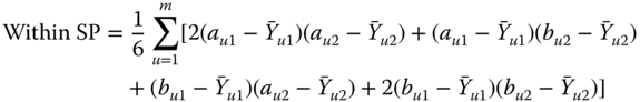
2.4.3 Sample Covariance and Correlation
When the number of variables ![]() , it is of interest to obtain measures of how these variables depend on each other. One such measure is the covariance. We note that for modal data it is necessary to know the corresponding probabilities for the pairs of each cross‐sub‐intervals in order to calculate the covariances. This is not an issue for interval data since there is only one possible cross‐interval/rectangle for each observation.
, it is of interest to obtain measures of how these variables depend on each other. One such measure is the covariance. We note that for modal data it is necessary to know the corresponding probabilities for the pairs of each cross‐sub‐intervals in order to calculate the covariances. This is not an issue for interval data since there is only one possible cross‐interval/rectangle for each observation.
As for the variance, we can show that the sum of products (SP) satisfies
where
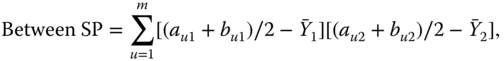

with ![]() obtained from Eq. 2.4.2.
obtained from Eq. 2.4.2.
As for the variance, we can show that Eq. 2.4.16 holds where now

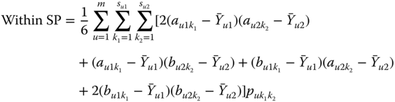

with ![]() obtained from Eq. 2.4.3.
obtained from Eq. 2.4.3.
2.4.4 Histograms
Brief descriptions of the construction of a histogram based on interval data and on histogram data, respectively, are presented here. More complete details and examples can be found in Billard and Diday (2006a).
Table 2.12 Airlines joint histogram (![]() ) (Example 2.16).
) (Example 2.16). ![]() = flight time in minutes,
= flight time in minutes, ![]() = arrival delay time in minutes
= arrival delay time in minutes
| 0.0246 | 0.0113 | 0.0143 | 0.0062 | 0.0808 | ||||||||||
| 0.1068 | 0.0676 | 0.0297 | 0.0412 | 0.0874 | ||||||||||
| 0.0867 | 0.0218 | 0.0132 | 0.0075 | 0.0220 | ||||||||||
| 0.0293 | 0.0166 | 0.0116 | 0.0106 | 0.0080 | ||||||||||
| 0.0328 | 0.0689 | 0.0388 | 0.0301 | 0.0714 | ||||||||||
| 0.0215 | 0.2293 | 0.1725 | 0.1950 | 0.2836 | ||||||||||
| 0.1013 | 0.0976 | 0.1047 | 0.0674 | 0.0933 | ||||||||||
| 0.0921 | 0.0802 | 0.0521 | 0.0443 | 0.0255 | ||||||||||
| 0.0398 | 0.0336 | 0.0535 | 0.0182 | 0.0172 | ||||||||||
| 0.0463 | 0.1011 | 0.1943 | 0.1503 | 0.0747 | ||||||||||
| 0.0070 | 0.0562 | 0.1726 | 0.0700 | 0.0390 | ||||||||||
| 0.0677 | 0.0449 | 0.0941 | 0.0430 | 0.0130 | ||||||||||
| 0.0925 | 0.0344 | 0.0023 | 0.0306 | 0.0288 | ||||||||||
| 0.0377 | 0.0711 | 0.0097 | 0.1126 | 0.0626 | ||||||||||
| 0.0449 | 0.0418 | 0.0186 | 0.0381 | 0.0314 | ||||||||||
| 0.0123 | 0.0235 | 0.0181 | 0.0270 | 0.0083 | ||||||||||
| 0.0420 | 0.0027 | 0.0045 | ||||||||||||
| 0.0558 | 0.0585 | 0.0210 | ||||||||||||
| 0.0258 | 0.0301 | 0.0217 | ||||||||||||
| 0.0330 | 0.0164 | 0.0057 | ||||||||||||
| 0.0079 | 0.0011 | 0.0152 | 0.0113 | 0.0120 | ||||||||||
| 0.0421 | 0.0675 | 0.0675 | 0.0249 | 0.0737 | ||||||||||
| 0.0147 | 0.0660 | 0.0262 | 0.0117 | 0.0556 | ||||||||||
| 0.0095 | 0.0363 | 0.0193 | 0.0120 | 0.0226 | ||||||||||
| 0.0076 | 0.0119 | 0.0179 | 0.0652 | 0.0226 | ||||||||||
| 0.0293 | 0.1259 | 0.0537 | 0.2258 | 0.1368 | ||||||||||
| 0.2793 | 0.1008 | 0.0207 | 0.0964 | 0.1729 | ||||||||||
| 0.1216 | 0.0463 | 0.0220 | 0.0709 | 0.0632 | ||||||||||
| 0.0568 | 0.0197 | 0.0758 | 0.0180 | 0.0135 | ||||||||||
| 0.0435 | 0.1173 | 0.1860 | 0.1096 | 0.1398 | ||||||||||
| 0.0095 | 0.1251 | 0.0978 | 0.0791 | 0.1474 | ||||||||||
| 0.0798 | 0.0886 | 0.0647 | 0.0520 | 0.0391 | ||||||||||
| 0.0473 | 0.0019 | 0.0468 | 0.0050 | 0.0195 | ||||||||||
| 0.0189 | 0.0038 | 0.1708 | 0.0239 | 0.0481 | ||||||||||
| 0.0161 | 0.0048 | 0.0826 | 0.0472 | 0.0331 | ||||||||||
| 0.0202 | 0.0119 | 0.0331 | 0.0413 | |||||||||||
| 0.0656 | 0.0314 | 0.0050 | ||||||||||||
| 0.0211 | 0.0868 | 0.0195 | ||||||||||||
| 0.0065 | 0.0400 | 0.0378 | ||||||||||||
| 0.0046 | 0.0130 | 0.0435 | ||||||||||||
| 0.0082 | ||||||||||||||
| 0.0446 | ||||||||||||||
| 0.0314 | ||||||||||||||
| 0.0077 | ||||||||||||||
| 0.0063 | ||||||||||||||
Table 2.13 Airlines joint histogram (![]() ) (Example 2.16).
) (Example 2.16). ![]() = flight time in minutes,
= flight time in minutes, ![]() = departure delay time in minutes
= departure delay time in minutes
| 0.0835 | 0.0227 | 0.0165 | 0.0106 | 0.0636 | ||||||||||
| 0.0532 | 0.0114 | 0.0319 | 0.0924 | |||||||||||
| 0.0381 | 0.0292 | 0.0242 | 0.0111 | 0.0423 | ||||||||||
| 0.0547 | 0.0122 | 0.0089 | 0.0120 | 0.0978 | ||||||||||
| 0.0273 | 0.1238 | 0.0079 | 0.0550 | 0.2361 | ||||||||||
| 0.0703 | 0.1844 | 0.0410 | 0.1543 | 0.1399 | ||||||||||
| 0.0789 | 0.1024 | 0.0896 | 0.0718 | 0.0312 | ||||||||||
| 0.0459 | 0.0654 | 0.1572 | 0.0559 | 0.0527 | ||||||||||
| 0.0681 | 0.0436 | 0.0454 | 0.0417 | 0.0600 | ||||||||||
| 0.0377 | 0.0889 | 0.0347 | 0.1246 | 0.0255 | ||||||||||
| 0.0525 | 0.0628 | 0.0583 | 0.0705 | 0.0546 | ||||||||||
| 0.0550 | 0.0405 | 0.0896 | 0.0448 | 0.0510 | ||||||||||
| 0.0472 | 0.0471 | 0.2377 | 0.0470 | 0.0116 | ||||||||||
| 0.0595 | 0.0615 | 0.0753 | 0.0971 | 0.0201 | ||||||||||
| 0.0357 | 0.0436 | 0.0535 | 0.0368 | 0.0213 | ||||||||||
| 0.0451 | 0.0187 | 0.0066 | 0.0275 | |||||||||||
| 0.0377 | 0.0068 | 0.0230 | ||||||||||||
| 0.0297 | 0.0181 | 0.0505 | ||||||||||||
| 0.0316 | 0.0088 | 0.0230 | ||||||||||||
| 0.0248 | 0.0084 | 0.0111 | ||||||||||||
| 0.0115 | 0.0214 | 0.0496 | 0.0072 | 0.0135 | ||||||||||
| 0.0227 | 0.0394 | 0.0551 | 0.0110 | 0.0526 | ||||||||||
| 0.0151 | 0.0499 | 0.0234 | 0.0154 | |||||||||||
| 0.0188 | 0.0534 | 0.0413 | 0.0186 | 0.0466 | ||||||||||
| 0.0136 | 0.0069 | 0.0427 | 0.0076 | 0.0662 | ||||||||||
| 0.0714 | 0.0252 | 0.0303 | 0.0976 | |||||||||||
| [0.1640 | 0.0648 | 0.0661 | 0.1411 | 0.1143 | ||||||||||
| 0.1195 | 0.0884 | 0.1887 | 0.0951 | |||||||||||
| 0.1121 | 0.0905 | 0.1694 | 0.0784 | 0.0541 | ||||||||||
| 0.0634 | 0.0159 | 0.1019 | 0.0460 | 0.0887 | ||||||||||
| 0.0194 | 0.0358 | 0.1639 | 0.0611 | 0.1158 | ||||||||||
| 0.0435 | 0.0897 | 0.0675 | 0.0721 | 0.0812 | ||||||||||
| 0.0468 | 0.1167 | 0.0444 | 0.0256 | |||||||||||
| 0.0377 | 0.0947 | 0.0450 | 0.0361 | |||||||||||
| 0.0241 | 0.0138 | 0.0359 | 0.0271 | |||||||||||
| 0.0216 | 0.0019 | 0.0148 | 0.0120 | |||||||||||
| 0.0432 | 0.0044 | 0.0202 | ||||||||||||
| 0.0278 | 0.0090 | 0.0302 | ||||||||||||
| 0.0170 | 0.0063 | 0.0265 | ||||||||||||
| 0.0084 | 0.0008 | 0.0258 | ||||||||||||
| 0.0104 | 0.0289 | 0.0192 | ||||||||||||
| 0.0292 | 0.0633 | 0.0183 | ||||||||||||
| 0.0295 | 0.0413 | 0.0195 | ||||||||||||
| 0.0210 | 0.0314 | 0.0214 | ||||||||||||
| 0.0082 | 0.0063 | 0.0274 | ||||||||||||
Table 2.14 Airlines joint histogram (![]() ) (Example 2.16).
) (Example 2.16). ![]() = arrival delay time in minutes,
= arrival delay time in minutes, ![]() = departure delay time in minutes
= departure delay time in minutes
| 0.0484 | 0.0667 | 0.0469 | 0.0434 | 0.1011 | ||||||||||
| 0.0139 | 0.0693 | 0.0343 | 0.0443 | 0.0912 | ||||||||||
| 0.0031 | 0.0122 | 0.0275 | 0.1157 | 0.0104 | ||||||||||
| 0.1349 | 0.1369 | 0.0002 | 0.3409 | 0.1101 | ||||||||||
| 0.1277 | 0.2345 | 0.0606 | 0.1006 | 0.2935 | ||||||||||
| 0.0476 | 0.0968 | 0.1156 | 0.0004 | 0.1257 | ||||||||||
| 0.0076 | 0.0009 | 0.2191 | 0.0155 | 0.0163 | ||||||||||
| 0.0601 | 0.0283 | 0.0107 | 0.0665 | 0.0640 | ||||||||||
| 0.0898 | 0.0702 | 0.0129 | 0.0962 | 0.1271 | ||||||||||
| 0.0865 | 0.0920 | 0.0447 | 0.0350 | 0.0021 | ||||||||||
| 0.0904 | 0.0270 | 0.1714 | 0.0027 | 0.0071 | ||||||||||
| 0.0002 | 0.0052 | 0.0787 | 0.0066 | 0.0513 | ||||||||||
| 0.0064 | 0.0139 | 0.0014 | 0.0164 | |||||||||||
| 0.0129 | 0.0371 | 0.0020 | 0.1157 | |||||||||||
| 0.0197 | 0.1090 | 0.0029 | ||||||||||||
| 0.0824 | 0.0191 | |||||||||||||
| 0.0113 | 0.0488 | |||||||||||||
| 0.0016 | 0.1030 | |||||||||||||
| 0.0039 | ||||||||||||||
| 0.0041 | ||||||||||||||
| 0.0334 | ||||||||||||||
| 0.1140 | ||||||||||||||
| 0.0267 | 0.0220 | 0.0689 | 0.0652 | 0.0135 | ||||||||||
| 0.0331 | 0.0314 | 0.0813 | 0.0318 | 0.0165 | ||||||||||
| 0.0145 | 0.0107 | 0.0055 | 0.0076 | 0.0165 | ||||||||||
| 0.0008 | 0.0019 | 0.1377 | 0.1090 | 0.0015 | ||||||||||
| 0.0904 | 0.0691 | 0.2562 | 0.1729 | 0.0917 | ||||||||||
| 0.2129 | 0.1601 | 0.0840 | 0.1043 | 0.1398 | ||||||||||
| 0.1545 | 0.1446 | 0.0510 | 0.0176 | 0.1023 | ||||||||||
| 0.0533 | 0.0275 | 0.0978 | 0.0230 | 0.0361 | ||||||||||
| 0.0003 | 0.0199 | 0.0785 | 0.0523 | 0.0496 | ||||||||||
| 0.0147 | 0.0627 | 0.0014 | 0.0828 | 0.1353 | ||||||||||
| 0.0486 | 0.1224 | 0.0152 | 0.1128 | 0.1564 | ||||||||||
| 0.0604 | 0.1310 | 0.1226 | 0.0013 | 0.0827 | ||||||||||
| 0.1069 | 0.0006 | 0.0028 | 0.0045 | |||||||||||
| 0.0055 | 0.0023 | 0.0057 | 0.0226 | |||||||||||
| 0.0025 | 0.0075 | 0.0101 | 0.0331 | |||||||||||
| 0.0068 | 0.0275 | 0.0595 | 0.0977 | |||||||||||
| 0.0074 | 0.1157 | 0.1414 | ||||||||||||
| 0.0378 | 0.0430 | |||||||||||||
| 0.0448 | ||||||||||||||
| 0.0002 | ||||||||||||||
| 0.0013 | ||||||||||||||
| 0.0019 | ||||||||||||||
| 0.0077 | ||||||||||||||
| 0.0670 | ||||||||||||||
2.5 Other Issues
There are very few theoretical results underpinning the methodologies pertaining to symbolic data. Some theory justifying the weights associated with modal valued observations, such as capacities, credibilities, necessities, possibilities, and probabilities (briefly described in Definitions 2.6–2.9), can be found in Diday (1995) and Diday and Emilion (2003). These concepts include the union and interception probabilities of Chapter , and are the only choice which gives Galois field sets. Their results embody Choquet (1954) capacities. Other Galois field theory supporting classification and clustering ideas can be found in Brito and Polaillon (2005).
The descriptive statistics described in section 2.4 are empirically based and are usually moment estimators for the underlying means, variances, and covariances. Le‐Rademacher and Billard (2011) have shown that these estimators for the mean and variance of interval data in Eqs. (2.4.2) and (2.4.5), respectively, are the maximum likelihood estimators under reasonable distributional assumptions; likewise, Xu (2010) has shown the moment estimator for the covariance in Eq. (2.4.15) is also the maximum likelihood estimator. These derivations involve separating out the overall distribution from the internal distribution within the intervals, and then invoking conditional moment theory in conjunction with standard maximum likelihood theory. The current work assumed the overall distribution to be a normal distribution with the internal variations following appropriately defined conjugate distributions. Implicit in the formulation of these estimators for the mean, variance, and covariance is the assumption that the points inside a given interval are uniformly spread across the intervals. Clearly, this uniformity assumption can be changed. Le‐Rademacher and Billard (2011), Billard (2008), Xu (2010), and Billard et al. (2016) discuss how these changes can be effected, illustrating with an internal triangular distribution. There is a lot of foundational work that still needs to be done here.
By and large, however, methodologies and statistics seem to be intuitively correct when they correspond to their classical counterparts. However, to date, they are not generally rigorously justified theoretically. One governing validity criterion is that, crucially and most importantly, methods developed for symbolic data must produce the corresponding classical results when applied to the special case of classical data.
Exercises
- 2.1 2.1
Show that the histogram data of Table 2.4 for
 = flight time have the sample statistics
  ,
,  and
and 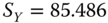 .
. - 2.2 2.2
Refer to Example 2.16 and use the data of Tables 2.12–2.14 for all
 airlines for
  = AirTime,
  = ArrDelay, and
  = DepDelay. Show that the sample statistics are
 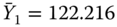 ,
,  ,
,  ,
,  ,
,  ,
,  ,
,  ,
,  ,
,  ,
,  ,
,  ,
,  .
.
Table 2.15 Airlines joint histogram (  ) (Exercise 3).
  = flight time in minutes,
  = arrival delay time in minutes


0.0246 

0.0113 

0.0032 

0.0062 

0.0808 
0.1068 
0.0676 
0.0408 
0.0412 
0.0940 
0.0867 
0.0218 
0.0132 
0.0075 
0.0154 
0.0293 
0.0166 
0.0116 
0.0106 
0.0080 
0.0328 

0.0689 

0.0088 

0.0301 

0.0714 

0.0215 
0.2293 
0.2025 
0.1950 
0.3155 
0.1013 
0.0976 
0.1047 
0.0674 
0.0614 
0.0921 
0.0802 
0.0521 
0.0443 
0.0255 
0.0398 

0.0336 

0.0157 

0.0182 

0.0172 
0.0463 
0.1011 
0.2320 
0.1503 
0.0846 

0.0070 
0.0562 
0.1726 
0.0700 
0.0291 
0.0677 
0.0449 
0.0941 
0.0430 
0.0130 
0.0925 

0.0344 

0.0005 

0.0306 

0.0288 
0.0377 
0.0711 
0.0114 
0.1126 
0.0709 
0.0449 
0.0418 
0.0186 
0.0381 
0.0232 

0.0123 
0.0235 
0.0181 
0.0270 
0.0083 
0.0420 

0.0027 

0.0045 
0.0558 
0.0585 
0.0279 
0.0258 
0.0301 
0.0149 
0.0330 
0.0164 
0.0057 

0.0079 

0.0011 

0.0193 

0.0022 

0.0120 
0.0421 
0.0675 
0.0634 
0.0340 
0.0737 
0.0147 
0.0660 
0.0262 
0.0117 
0.0556 
0.0074 
0.0363 
0.0096 
0.0120 
0.0226 
0.0046 

0.0119 
0.0096 

0.0110 

0.0226 
0.0050 
0.1259 

0.0179 
0.2800 
0.1368 

0.0293 
0.1008 
0.0537 
0.0964 
0.1729 
0.2793 
0.0463 
0.0207 
0.0709 
0.0632 
0.1216 

0.0197 
0.0138 

0.0013 

0.0135 
0.0462 
0.1173 
0.0083 
0.1263 
0.1398 
0.0238 
0.1251 

0.0813 
0.0791 
0.1474 
0.0303 
0.0886 
0.1804 
0.0520 
0.0391 

0.0095 

0.0019 
0.0978 

0.0003 

0.0000 
0.0798 
0.0038 
0.0234 
0.0287 
0.0195 
0.0473 
0.0048 
0.0413 
0.0472 
0.0481 
0.0156 
0.0119 

0.0565 
0.0413 
0.0331 
0.0079 

0.0314 
0.1612 

0.0013 
0.0115 
0.0868 
0.0826 
0.0233 

0.0202 
0.0400 
0.0207 
0.0378 
0.0656 
0.0130 
0.0124 
0.0435 
0.0211 
0.0062 
0.0013 
0.0036 

0.0082 
0.0446 
0.0314 
0.0065 
0.0030 
0.0046 Table 2.16 Airlines joint histogram (
 ) (Exercise 3).
  = flight time in minutes,
  = departure delay time in minutes


0.0835 

0.0227 

0.0165 

0.0106 

0.0636 
0.0767 
0.0532 
0.0114 
0.0319 
0.0924 
0.0381 
0.0292 
0.0224 
0.0111 
0.0423 
0.0547 
0.0122 
0.0107 
0.0120 

0.0978 
0.0273 

0.1238 
0.0079 

0.0550 
0.2361 

0.0703 
0.1844 

0.0410 
0.1543 
0.1399 
0.0789 
0.1024 
0.0896 
0.0718 

0.0312 
0.0459 
0.0654 
0.1447 
0.0559 
0.0527 
0.0681 

0.0436 
0.0580 

0.0417 
0.0600 
0.0377 
0.0889 
0.0347 
0.1246 

0.0255 

0.0525 
0.0628 

0.0583 
0.0705 
0.0546 
0.0550 
0.0405 
0.0896 
0.0448 
0.0510 
0.0472 

0.0471 
0.2165 

0.0470 

0.0116 
0.0595 
0.0615 
0.0966 
0.0971 
0.0201 
0.0357 
0.0436 
0.0535 
0.0368 
0.0213 

0.0451 
0.0187 

0.0066 
0.0275 
0.0377 
0.0068 

0.0230 
0.0297 
0.0161 
0.0505 
0.0316 
0.0107 
0.0230 
0.0248 
0.0084 
0.0111 

0.0115 

0.0214 

0.0496 

0.0072 

0.0135 
0.0227 
0.0394 
0.0551 
0.0110 
0.0526 
0.0151 
0.0499 
0.0234 
0.0154 
0.0511 
0.0188 
0.0534 

0.0413 
0.0186 
0.0466 
0.0136 
0.0069 
0.0427 
0.0076 

0.0662 

0.0714 

0.0252 
0.0303 

0.0976 
0.1368 
0.1640 
0.0648 

0.0661 
0.1411 
0.1143 
0.1195 
0.0884 
0.1887 
0.0951 
0.0782 
0.1121 
0.0905 
0.1694 
0.0784 

0.0541 
0.0634 
0.0159 

0.1019 
0.0460 
0.0887 

0.0194 

0.0358 
0.1639 

0.0611 
0.1158 
0.0435 
0.0897 
0.0675 
0.0721 
0.0812 
0.0468 
0.1167 
0.0444 

0.0256 
0.0377 
0.0947 
0.0450 
0.0361 
0.0241 
0.0138 
0.0359 
0.0271 

0.0216 

0.0019 

0.0148 
0.0120 
0.0432 
0.0044 
0.0202 
0.0278 
0.0090 
0.0302 
0.0170 
0.0063 
0.0265 
0.0084 
0.0008 
0.0258 

0.0104 

0.0289 

0.0192 
0.0292 
0.0633 
0.0183 
0.0295 
0.0413 
0.0195 
0.0210 
0.0314 
0.0214 
0.0082 
0.0063 
0.0274 Table 2.17 Airlines joint histogram (
 ) (Exercise 3).
  = arrival delay time in minutes,
  = departure delay time in minutes


0.0277 

0.1116 

0.0469 

0.0434 

0.1011 
0.0328 
0.1373 
0.0343 
0.0443 
0.0912 
0.0049 
0.0275 
0.0275 

0.1157 
0.0104 

0.0595 

0.0920 
0.0002 
0.3409 

0.1101 
0.1837 
0.1665 

0.0606 
0.1006 
0.2935 
0.0718 
0.0815 
0.1156 
0.0004 
0.1257 
0.0029 
0.0009 
0.2191 

0.0155 

0.0163 

0.0273 

0.0283 
0.0107 
0.0665 
0.0640 
0.0960 
0.0702 

0.0129 
0.0962 
0.1271 
0.1171 
0.0920 
0.0447 
0.0350 

0.0021 
0.0457 
0.0270 
0.1714 

0.0027 
0.0071 

0.0037 

0.0052 
0.0787 
0.0066 
0.0513 
0.0207 
0.0139 
0.0014 
0.0164 
0.0459 
0.0371 

0.0020 
0.1157 
0.1007 
0.1090 
0.0025 
0.0027 
0.0168 

0.0006 
0.0463 
0.0037 
0.0504 
0.0076 

0.0004 
0.0515 
0.0023 
0.0937 
0.0025 
0.0526 

0.0267 

0.0220 

0.0702 

0.0652 

0.0135 
0.0331 
0.0314 
0.0829 
0.0318 
0.0165 
0.0145 
0.0107 
0.0056 
0.0076 
0.0165 
0.0008 
0.0019 

0.1320 

0.1090 
0.0015 

0.0904 

0.0691 
0.2528 
0.1729 

0.0917 
0.2129 
0.1601 
0.0829 
0.1043 
0.1398 
0.1545 
0.1446 

0.0520 
0.0176 
0.1023 
0.0533 
0.0275 
0.0997 

0.0230 
0.0361 
0.0003 

0.0199 
0.0801 
0.0523 

0.0496 

0.0147 
0.0627 

0.0014 
0.0828 
0.1353 
0.0486 
0.1224 
0.0154 
0.1128 
0.1564 
0.0604 
0.1310 
0.1250 
0.0013 
0.0827 
0.1069 
0.0006 

0.0028 

0.0045 
0.0055 

0.0023 
0.0057 
0.0226 

0.0025 
0.0075 
0.0101 
0.0331 
0.0068 
0.0275 
0.0595 
0.0977 
0.0074 
0.1157 
0.1414 
0.0378 
0.0430 
0.0448 

0.0002 
0.0013 
0.0019 
0.0077 
0.0670 - 2.3
2.3
Consider the airline data with joint distributions in Tables 2.15–2.17.
- Using these tables, calculate the sample statistics
 ,
,  ,
,  and
and  ,
,  .
. - How do the statistics of (a) differ from those of Exercise 2.2, if at all? If there are differences, what do they tell us about different aggregations?
- Using these tables, calculate the sample statistics