
Chapter 12
Design and Development of Multivariate Diagnostic Systems
12.0 Introduction
In previous chapters, we have described the importance of data quality and how it can be measured and improved with the critical data element (CDE) view. After ensuring high-quality and reliable data, the data should be used in a meaningful way to derive important insights. The methodology described in this chapter is useful in ensuring high information quality that will help up us to formulate important insights. We usually have to deal with the information based on more than one variable or CDE in order to draw insights, which will need to be used in relation to one another to make important decisions. Systems with more than one CDE or variable can be called multivariate systems. Examples of multivariate systems include medical diagnosis systems, client relationship mechanisms, fraud detection systems, and fire alarm sensor systems. This chapter describes the Mahalanobis-Taguchi Strategy (MTS) and its applicability to developing a multivariate diagnostic system with a measurement scale. The Mahalanobis distance (MD) is used to measure the distances in a multivariate system, and Taguchi's principles are used to measure accuracy of the system and identify important variables that are sufficient for the measurement system. This methodology is becoming increasingly popular, evidenced by the many case applications around the globe.
12.1 The Mahalanobis-Taguchi Strategy
The Mahalanobis-Taguchi Strategy (MTS) is a pattern analysis technique, which is used to conduct system diagnosis through a multivariate measurement scale. In multivariate systems, patterns are difficult to represent in quantitative terms and they are extremely sensitive to correlations between the variables. The importance of correlations in multivariate systems is illustrated by Figure 12.1.
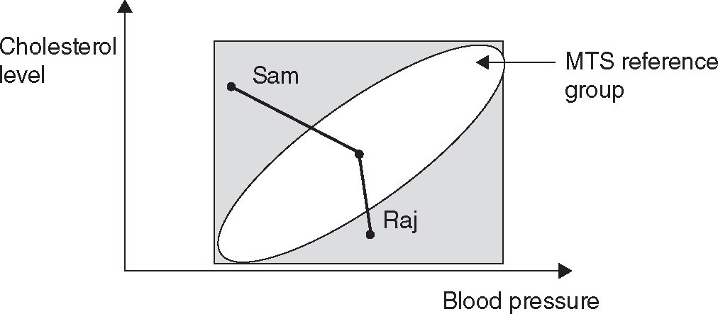
Figure 12.1 Importance of Correlations in Multivariate Systems
In Figure 12.1, if we look at the variable blood pressure and cholesterol levels independently of each other, then we can conclude that both Sam and Raj are normal (within the rectangular area). However, if we consider the correlations between the variables, then we can say that they are somewhat abnormal, as they do not fall within the elliptical area that forms the reference group. Furthermore, we can precisely state that Sam is sicker than Raj, since his distance from the center of the ellipse is larger than that of Raj. Through MTS analysis, we can obtain such insights by expressing patterns in quantitative terms.
The Mahalanobis distance (MD), which was introduced by well-known Indian statistician P. C. Mahalanobis, measures distances of points in multidimensional spaces. Taguchi methods have been successfully applied in many engineering applications to improve the performance of the products/processes/systems. They are proved to be extremely useful and cost effective. In the context of MTS, following two aspects of Taguchi methods are used:
- Signal to noise ratios or S/N ratios: they are used to measure the accuracy of MTS diagnostic system
- Orthogonal arrays: they are used to optimize the diagnostic systems by minimizing the number of variable combinations to study.
In the subsequent sections of this chapter, a detailed discussions on S/N ratios and orthogonal arrays in relation to MTS have been provided.

Figure 12.2 The Gram-Schmidt Process
The Mahalanobis distance has been used extensively in several areas such as spectrographic applications and agricultural applications. Because it takes correlations between the variables into account, the Mahalanobis distance has proved to be superior to other multidimensional distances such as the Euclidean distance. The Mahalanobis distance is calculated by using the following equation:
- Zi = standardized vector of Xi (i = 1 . . . k),
- C = correlation matrix, and
- k = number of CDEs/variables
The Mahalanobis distance can also be calculated by using the Gram-Schmidt orthogonalization process. The Gram-Schmidt process (GSP) can simply be stated as follows: Given linearly independent vectors Z1, Z2, . . . , Zk, there exist mutually perpendicular vectors U1, U2, . . . , Uk with the same linear span. This process is described in Figure 12.2.
12.1.1 The Gram Schmidt Orthogonalization Process
Given linearly independent vectors Z1,Z2, . . . Zk, there exist mutually perpendicular vectors U1,U2, ... Uk with the same linear span (Figure 12.2).
The Gram-Schmidt vectors are constructed sequentially by setting:

where ' denotes transpose of a vector. When calculating MD using the GSP, standardized values for the variables are used. Therefore, in the preceding set of equations Z1, Z2, . . . Zk correspond to standardized values. From this set of equations, it is clear that the transformation process depends largely on the first variable.
Calculation of MD using Gram Schmidt's Orthogonalization Process
Suppose we have a sample of size n, and each sample contains observations on k variables. After standardizing the variables, we will have a set of standardized vectors. Let these vectors be as follows:
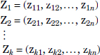
After performing GSP, we have orthogonal vectors as follows:
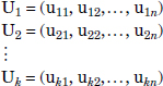
It easily follows that the mean of vectors U1, U2, . . . , Uk is zero. Let s1, s2, . . . sk be standard deviations (s.d.s) of U1,U2, . . . ,Uk, respectively. Since we have a sample of size n, there will be n different MDs. The MD corresponding to the jth observation of the sample is computed using Equation (12.3).
where j = 1 . . . n. The values of MD obtained from Equations (12.1) and (12.3)> are exactly the same, and this can be proved easily.
The most important consideration for developing a multivariate measurement system using the Mahalanobis distance is to have a reference point. While it is easier to obtain a reference point for the scale with a single characteristic, it is not so easy to obtain a single reference point when we are dealing with multiple characteristics. Therefore, in MTS, the reference point corresponding to multiple variables is obtained with the help of a group of observations that are as uniform as possible and still enable us to distinguish their different patterns through the MD. These observations are modified in such a way that their center is located at the origin and the corresponding Mahalanobis distances are scaled so as to make the average distance of this group unity. The set of observations used for the reference is often referred to as the Mahalanobis space (MS) or reference group or normal group. Selection of this group is entirely at the discretion of the decision maker conducting the diagnosis. In fraud analytics, this group can be one where there are no incidences of fraud; in a medical diagnosis application, this group can be a set of people without any health problems; and in stock market predictions, this group could correspond to companies having average steady growth in a three-year period. The observations in this group are similar but not the same. Judicious selection of this group is extremely important for accurate diagnosis or predictions.
After developing the scale, the next step is the validation of the scale, which is done with the help of observations that are outside the Mahalanobis space. If the scale is good, the distances of these observations must be consistent with the decision maker's judgment. In other words, if an observation does not belong to the reference group, then it should have a larger distance. To quantify the diagnostics accuracy, we typically use a signal-to-noise (S/N) ratio metric. S/N ratio captures the magnitude of real effects after making some adjustment for uncontrollable variation (noise) by taking into account the correlation between the true or observed information (i.e., input signals) and the output of the diagnostic system (the Mahalanobis distance). In a multivariate context, S/N ratio can simply be defined as the measure of the accuracy of the diagnostics. A typical multidimensional predictive system that is used in MTS can be described using Figure 12.3.
As mentioned, the output or diagnosis accuracy should correlate well with the input signal, and S/N ratios measure this correlation. The diagnostics are conducted based on the information on the variables defining the system, and they should be “accurate” even in the presence of noise factors such as different places of measurement, operating conditions, and so forth.
If the accuracy of the diagnosis is satisfactory, then we identify a useful subset of variables that is sufficient for the measurement scale with acceptable diagnostic accuracy. Experience shows that, in many cases, the accuracy with useful variables is better than that with the original set of variables. However, in some cases, the accuracy with useful variables might be less—which might still be desirable, as it helps reduce the cost of inspection or measurement. In multidimensional systems, the total number of combinations to be examined would be of the order of several thousands; hence, it is not possible to examine all combinations. Here, we propose use of orthogonal arrays (OAs) to reduce the number of combinations to be tested. OAs are developed to estimate the effects of the variables by minimizing the number of combinations to be examined. They have been in use for quite a long time in the field of experimental design. In MTS, the variables are assigned to different columns of an OAs. Based on S/N ratios obtained from different variable combinations, important variables are identified. The future diagnosis is carried out only with these important variables.

Figure 12.3 Pattern Information or Diagnostic System Used in MTS
12.2 Stages in MTS
From the preceding discussion, the basic stages in MTS can be summarized as follows:
Stage I: Develop Measurement Scale
- Select a Mahalanobis space or reference group with suitable variables and observations that are as uniform as possible.
- Use the Mahalanobis space as a base or reference point of the scale.
Stage II: Validate Measurement Scale
- Identify the conditions outside the Mahalanobis space.
- Compute the Mahalanobis distances of these conditions and check whether they are consistent with the decision maker's judgment.
Stage III: Optimize Measurement Scale
- Optimize the scale by identifying the useful set of variables using orthogonal arrays and signal-to-noise ratios.
Stage IV: Conduct Future Diagnosis
- Monitor the conditions using the scale developed with the help of the useful set of variables. Based on the values of Mahalanobis distances, take appropriate corrective actions.
Figure 12.4 shows the different steps in MTS.
From the preceding discussion, it is clear that orthogonal arrays play a prominent role in the third stage of MTS analysis. Each experimental run in the orthogonal array design matrix uses a subset of variables; the resulting S/N ratios of these subsets are calculated using the distances outside of the reference group.
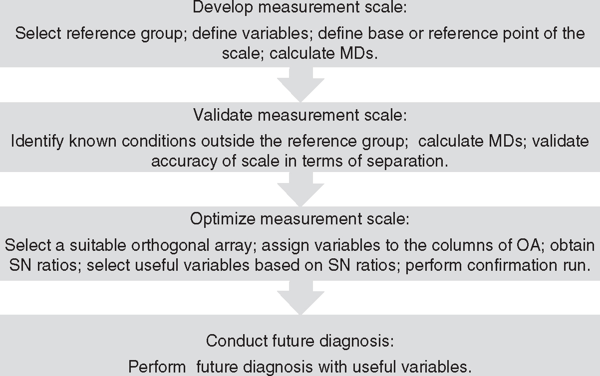
Figure 12.4 Steps in MTS
12.3 The Role of Orthogonal Arrays and Signal-to-Noise Ratio in Multivariate Diagnosis
In the context of MTS, orthogonal arrays are used to estimate the effects of several factors and the effect of interactions by minimizing the number of experiments, and signal-to-noise ratio is used as a measure of diagnosis accuracy. Use of S/N ratios ensures a high level of prediction with useful variables. S/N ratios are computed for all combinations of the orthogonal array using Mahalanobis distances. S/N ratios are also used to select important variables for future diagnosis. Using S/N ratios as the response, average effects of variables are computed at level 1 (presence) and level 2 (absence). Based on these effects, the importance of variables can be determined. The examples provided in this chapter show how we can make such determinations.
12.3.1 The Role of Orthogonal Arrays
In robust engineering, the main role of OAs is to permit engineers to evaluate a product design with respect to robustness against noise and the cost involved. OA is an inspection device to prevent a poor design from going downstream.
Usually, these arrays are denoted as La(bc)
- a = number of experimental runs
- b = number of levels of each factor
- c = number of columns in the array
- L denotes Latin square design
Arrays can have factors with many levels, although two- and three-level factors are most commonly encountered.
In the MTS, orthogonal arrays are used to select the variables of importance by minimizing the different combinations of the original set of variables. The variables are assigned to the different columns of the array. The presence and absence of the variables are considered the levels. Since the variables have only two levels, two-level arrays are used in MTS application. The importance of the variables is judged based on their ability to measure the degree of abnormality on the measurement scale. For each run of an OA, the MDs corresponding to the known abnormal conditions or the conditions outside the MS are computed. We need not consider the MDs corresponding to the reference group because we know that this group is healthy and, based on this group, scale is constructed.
For the purpose of illustration, consider the following example.
Let there be five variables X1, X2, X3, X4, and X5. Let us allocate these variables in the first five columns of the L8(27) array, as shown in Table 12.1. In this table, “1” indicates the level corresponding to the presence of a variable and “2” indicates the level corresponding to the absence of a variable. Consider the first three runs of Table 12.1.
1st Run: 1-1-1-1-1
In this run, the MS is constructed with the variable combination X1-X2-X3-X4-X5. The correlation matrix is of the order 5 × 5. The MDs of abnormals are estimated with this matrix.
2nd Run: 1-1-1-2-2
In this run, the MS is constructed with the variable combination X1-X2-X3. The correlation matrix is of the order 3 × 3. The MDs of abnormals are estimated with this matrix.
Table 12.1 Variable Allocation in L8(27) Array

3rd Run: 1-2-2-1-1
In this run, the MS is constructed with the variable combination X1-X4-X5. The correlation matrix is of the order 3 × 3. The MDs of abnormals are estimated with this matrix.
Based on the MDs of the conditions, outside the MS, corresponding to the runs of an orthogonal array, we can evaluate S/N ratios. Thus, OAs are required for testing the different combinations of the variables to identify the variables of importance based on their ability to measure the conditions outside the MS.
12.3.2 The Role of S/N Ratios in MTS
The S/N ratio tries to capture the magnitude of true information (i.e., signals) after making some adjustment for uncontrollable variation (i.e., noise).
In the case of multivariate diagnosis, the S/N ratio is defined as the measure of the accuracy of the measurement scale for predicting abnormal conditions. S/N ratio is expressed in decibel (dB) units. A higher value for the S/N ratio means lower error of prediction. Note that S/N ratios are calculated using abnormal conditions only, as it is required that the accuracy of the scale be tested based on these conditions.
In multidimensional applications, it is important to identify a useful set of variables that is sufficient to detect the abnormals. It is also important to assess the performance of the given system and the degree of improvement in the performance. In this method, S/N ratios are used to accomplish these objectives.
After obtaining the MDs for the known abnormal conditions corresponding to the various combinations of an OA, S/N ratios are computed for all these combinations to determine the useful set of variables. S/N ratios are important to improve the accuracy of the measurement scale and reduce the cost of diagnosis. The useful set of variables is obtained by evaluating the gain in the S/N ratio, which is the difference between the average S/N ratio when the variable is used in an OA and the average S/N ratio when the variable is not used in an OA. If the gain is positive, then the variable is useful.
12.3.3 Types of S/N Ratios
In MTS application, typically the following types of S/N ratios are used:
- Larger-the-better type
- Nominal-the-best type
- Dynamic type
When the true levels of abnormals are not known, the larger-the-better type of S/N ratios is used if all the observations outside the reference group are abnormals. This is because the MDs for abnormals should be higher. If the observations outside the reference group are a mixture of normals and abnormals, then the nominal-the-best type of S/N ratios is used. When the levels of abnormals are known, the dynamic type of S/N ratios is used. In some cases, it is quite difficult to obtain the levels of severity of the abnormals based on the knowledge of the person conducting the diagnosis. In such situations, if we know the abnormals with different degrees of severity (different categories), dynamic S/N ratios can be used by taking the average of the square root of the MDs (working average) in each category as known levels of abnormals.
Equations for S/N Ratios
Larger-the-Better Type
The procedure for calculating S/N ratios corresponding to a run of an OA is as follows:
Let there be t abnormal conditions. Let D12, D22, . . . , Dt2 be MDs corresponding to the abnormal situations. The S/N ratio (for the larger-the-better criterion) corresponding to the qth run of an OA is given by the following:
Nominal-the-Best Type
The procedure for calculating S/N ratios corresponding to a run of an OA is as follows:
Let there be t abnormal conditions. Let D12, D22, . . . , Dt2 be MDs corresponding to the abnormal situations. The S/N ratio (nominal-the-better type) corresponding to the qth run of an OA is calculated as follows:
where ![]() is the average of the Dis
is the average of the Dis
Dynamic Type
An examples of the dynamic type is a weather forecasting system and the specific case of rainfall prediction. The procedure for calculating S/N ratios corresponding to a run of an OA is as follows:
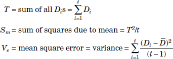
Let there be t abnormal conditions. Let D12, D22, . . . , Dt2 be the MDs corresponding to the abnormal conditions. Let M1, M2, . . . , Mt be the true levels of severity (rainfall values in the rainfall prediction system example).
For each run of the OA, construct the following ANOVA table:
| Source | Degrees of Freedom | Sum of Squares |
| β | 1 | Sβ |
| e | T − 1 | Se |
| Total | T | ST |
In the preceding ANOVA table,
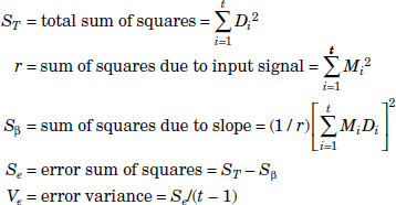
The S/N ratio corresponding to the qth run of OA is given by the following:
In the case of working average methods, true levels of severity (M) are replaced by the average of the square root of MDs.
12.3.4 Direction of Abnormals
One of the main reasons for using the Mahalanobis distance in multivariate diagnosis is its capability of distinguishing abnormalities from a “healthy” or “normal” group. Sometimes, the abnormal conditions arise out of extremely good situations. Therefore, it is important to identify the direction of the abnormalities to enable the distinction between “good” and “bad” abnormalities to be made. This makes the diagnosis process more effective. If the MD is calculated by using the inverse of the correlation matrix (the MTS method), such distinctions cannot be made. However, this can be accomplished if we use the Gram-Schmidt orthogonalization process to calculate the MD. This section outlines a procedure for identifying the direction of abnormals with suitable equations for different cases. The use of this procedure is demonstrated for a graduate student admission system.
The GSP vectors obtained from Equation (12.2) can be written as:
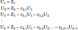
where c2,1, c2,1, . . . , ck,k−1 are Gram-Schmidt vector coefficients.
First, a discussion of the direction of abnormals is presented in detail for a two-variable case. The same logic is extended for a higher number of variables.
In the case of two variables, the distribution of the points forms an elliptical shape. Since the MS is constructed based on this distribution, for simplicity, we can represent this distribution as the MS. It is a well-known fact that the elliptical shape remains unchanged after orthogonal transformation. Therefore, the distribution corresponding to the GSP vectors will also have an elliptical shape.
We know that the mean of the GSP vectors is located at the zero point. For the two-variable case, the mean of U1 and U2 is located at (0,0). All conditions (normal and abnormal) are above or below this point with the exception of the points that match the zero point (mean). Therefore, it is clear that the abnormals are above or below the zero point. Based on the position of the abnormals (above or below zero point) and the value of the MD, we can distinguish between “good” and “bad” abnormals. In the case of two variables, depending on the types of characteristics, we have the following four cases:
- Both U1 and U2: larger-the-better type
- U1: smaller-the-better type; U2: larger-the-better type
- U1: larger-the-better type; U2: smaller-the-better type
- Both U1 and U2: smaller-the-better type
For a two-variable case, the vectors U1 and U2 can be written as follows:
or
For all four of these cases, the rules for identifying the direction of abnormals are described in the following sections.
Case 1: Both U1 and U2—Larger-the-Better Type
An example where the characteristics U1 and U2 are of the larger-the-better type is a student admission system. In this system, U1 could be “GPA” (grade point average) and U2 could be “TOEFL exam score.” In this case, a condition corresponding to very low U1 and U2 is an abnormal, and a condition corresponding to very high U1 and U2 is also an abnormal.
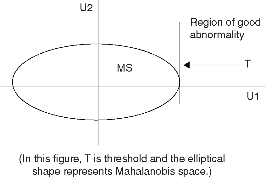
Figure 12.5 Both U1 and U2 are Larger-the-Better Type
For the jth condition to be a good-abnormal, the elements of U1 and U2 should be above zero (positive) and the corresponding MD should be larger than the threshold (T). These conditions can be mathematically represented as:
- u1j > 0 or z1j > 0; u2j > 0 or z2j − c2,1 u1j > 0 or z2j > c2,1 u1j and
- MDj > T
From Equation (12.3), we can write:
The pictorial representation of these rules is given in Figure 12.5.
For this case, the decision rule can be stated as follows: If elements of U1 and U2 corresponding to an abnormal condition are positive and MD is higher than the threshold (T), then the abnormal condition can be classified as “good” abnormality; otherwise, it is a “bad” abnormality.
Case 2: U1—Smaller-the-Better Type and U2—Larger-the-Better Type
An example of this situation is the banking system for granting loans.Here, U1 could be “number of people in a household” and U2 could be “income level of a family.” In this case, a condition corresponding to very high U1 and very low U2 is an abnormal, and a condition corresponding to very low U1 and very high U2 is also an abnormal.

Figure 12.6 U1—Smaller-the-Better Type and U2—Larger-the-Better Type
For the jth condition to be a good-abnormal, the element of U1 should be below zero (negative) and that of U2 should be above zero (positive) and the corresponding MD should be larger than the threshold (T). These conditions can be mathematically represented as follows:
- u1j < 0 or z1j < 0; u2j > 0 or z2j − c2,1 u1j > 0 or z2j > c2,1 u1j and
- MDj > T
From Equation (12.3), we can write:
The pictorial representation of these rules is given in Figure 12.6.
For this case, the decision rule can be stated as follows: If the element of U1 is negative and that of U2 is positive and MD is higher than the threshold (T), then the abnormal condition can be classified as “good” abnormality; otherwise, it is “bad” abnormality.
Case 3: U1—Larger-the-Better Type and U2—Smaller-the-Better Type
An example of this situation is an inspection system, where the characteristic “tensile strength” (U1) is of the larger-the-better type and the characteristic “number of occurrences of a particular defect” (U2) is of the smaller-the-better type. In this case, a condition corresponding to very low U1 and very high U2 is an abnormal, and a condition corresponding to very high U1 and very low U2 is also an abnormal.
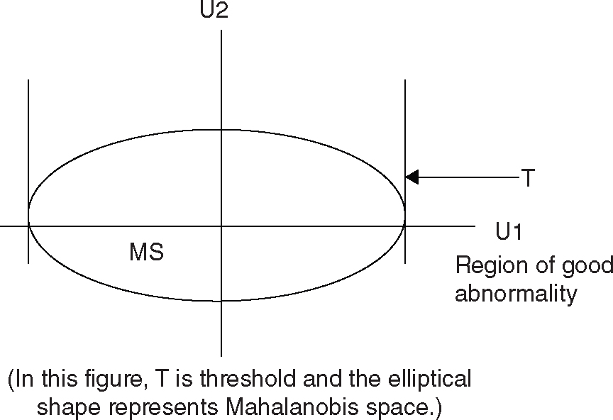
Figure 12.7 U1—Larger-the-Better Type and U2—Smaller-the-Better Type
For the jth condition to be a good-abnormal, the element of U1 should be above zero (positive) and that of U2 should be below zero (negative) and the corresponding MD should be larger than threshold (T). These conditions can be mathematically represented as follows:
- u1j > 0 or z1j > 0; u2j < 0 or z2j − c2,1 u1j < 0 or z2j > c2,1 u1j and
- MDj > T
From Equation (12.3), we can write:
The pictorial representation of these rules is given in Figure 12.7.
For this case, the decision rule can be stated as follows: If the element of U1 is positive and that of U2 is negative and MD is higher than the threshold (T), then the corresponding abnormal condition can be classified as “good” abnormality; otherwise, it is a “bad” abnormality.
Case 4: Both U1 and U2 Are Smaller-the-Better Type
An example of a situation where both the characteristics are of the smaller-the-better type is a printed circuit board inspection system. In this example, the characteristics “number of occurrences of a particular defect” (U1) and “line width reduction after etching process” (U2) are of the smaller-the-better type. In this case, a condition corresponding to very high U1 and U2 is an abnormal, and a condition corresponding to very low U1 and U2 is also an abnormal.
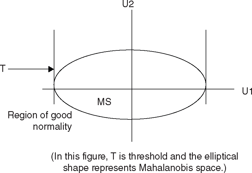
Figure 12.8 Both U1 and U2 Are Smaller-the-Better Type
For the jth condition to be a good-abnormal, the elements of U1 and U2 should be below zero (negative) and the corresponding MD should be larger than the threshold (T). These conditions can be mathematically represented as follows:
- u1j < 0 or z1j < 0; u2j < 0 or z2j − c2,1 u1j < 0 or z2j < c2,1 u1j and
- MDj > T
From Equation (12.3), we can write:
The pictorial representation of these rules is given in Figure 12.8.
For this case, the decision rule can be stated as follows: If the elements of U1 and U2 corresponding to an abnormal condition are negative and MD is higher than the threshold (T), then the abnormal condition can be classified as “good” abnormality; otherwise, it is a “bad” abnormality.
Decision Rule for Higher Dimensions
If there are k variables and the sample size is n, the conditions for the jth abnormal to be good are:
- u1j > 0, if U1 is larger-the-better type (<0 if U1 is smaller-the-better type)
- u2j > 0, if U2 is larger-the-better type (<0 if U2 is smaller-the-better type)

- ukj > 0, if Uk is larger-the-better type (<0 if Uk is smaller-the-better type)
and
or
otherwise, the abnormal condition is bad.
Though this procedure provides guidelines for identifying the direction of abnormals, it is left to the decision maker to decide the type of abnormal conditions. For example, in a student admission system, where the variables are mostly of the higher-the-better type, a student with very high scores on most of the variables can be considered a good-abnormal by the decision maker.
It is important to note that this procedure is applicable only to cases where we have knowledge about the type of variables (such as larger-the-better type or smaller-the-better type).
Graduate Admission System Example
The applicability of this procedure can be demonstrated using the example of a university student admission system. Suppose a student is admitted into the university based on the following three variables:
- Grade point average (GPA): This should be as high as possible on a 4.0 scale.
- GMAT score: This should be as high as possible (maximum score is 1600).
- SAT-Math score: This should be as high as possible (maximum score is 800).
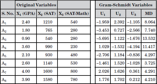
The data corresponding to the reference group along with GSP vectors and MDs are shown in Table 12.2. Since these variables are of the larger-the-better type, this example falls into the first category. There are eight abnormal conditions A1 . . . A8. The abnormal data along with GSP vectors and MDs are given in Table 12.3.
From Table 12.3, it is clear that all of the abnormalities have high MDs. Based on MDs alone, we cannot distinguish between good and bad abnormalities. To make such distinctions, we need to look at GSP vectors. Assuming the threshold (T) is set at 3.0, A7 and A8 can be classified as “good” abnormalities because GSP vectors corresponding to these abnormalities have positive signs and their MDs are higher than threshold. The remaining abnormalities (A1 to A6) can be classified as “bad” abnormalities because not all corresponding GSP vectors have positive signs even though their MDs are higher than threshold.
Table 12.2 Analysis of Reference Group Data

Table 12.3 Analysis of Abnormal Data
12.4 A Medical Diagnosis Example
This example involves a liver disease diagnosis that was carried out by Dr. Kanetaka. The variables considered for the purpose of the diagnosis are as shown in Table 12.4. The healthy group, or reference group, was constructed based on observations of 200 people who did not have any health problems. There were 17 patients with known liver disease problems (these are referred to as abnormal). For this application, different stages of the MTS were applied as described. Figure 12.9 clearly shows the separation between normals and abnormals, indicating the ability of the scale to differentiate between the reference group and the abnormals, which is sufficient to validate the scale.
Table 12.4 Variables in Medical Diagnosis Data
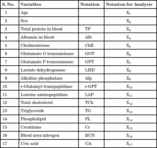
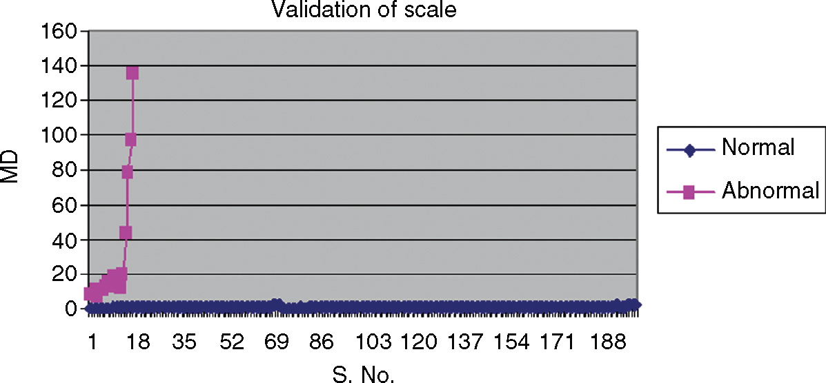
Figure 12.9 Differentiation between Normals and Abnormals (validation of the scale)
Next is the optimization phase. In this phase, the useful set of variables was identified using OAs and S/N ratios. Since there are 17 variables and we required a two-level OA, an L32(231) array was selected. L32(231) array is a two-level OA with 32 treatment combinations (runs) and 31 columns. A list of orthogonal arrays is provided in Appendix C. The 17 variables were allocated to the first 17 columns of this array. The MDs corresponding to the 17 abnormal conditions were computed for all 32 combinations of the variables, and dynamic S/N ratios were calculated. The S/N ratios were obtained by using the procedure given in the Section 12.3. The average responses corresponding to the 17 variables are shown in Table 12.5.
In Table 12.5, Level 1: variable is present; Level 2: variable is not present.
From Table 12.5, it is clear that the variables X4, X5, X10, X12, X13, X14, X15, and X17 have positive gains. That means these variables have higher average responses when they are part of the system (Level 1). Hence, these variables were considered to be useful for a future diagnosis process. The results of the confirmation run showed that the measurement scale (developed with useful variables) can detect the abnormals. This can also be seen from Figure 12.10.
Table 12.5 Average Responses for Dynamic S/N Ratios (in dB units)
For a full-size version of this table go to www.wiley.com/go/highqualitydata.


Figure 12.10 Normals and Abnormals after Optimization
It was also found that the average MD of abnormal conditions with useful variables was higher than that with all the variables. This means the insignificant variables will reduce the accuracy of the MD. Since the gain in S/N ratio for X4 is very small, a combination of the useful variables excluding X4 is run to check the performance of the system. It was found that abnormals have lower MDs with this combination. Therefore, it was decided to retain X4 in the set of useful variables.
12.5 Case Study: Improving Client Experience
This example concerns a financial institution. Following is a summary of this case.
This study focused on improving the measurement of key indicators of client relationship health. The client health was decided based on 49 variables and classified into green (loyal), yellow (vulnerable), and red (at-risk) groups of clients. Prior to this study, the decisions were made based on the client relationship manager's judgment without having any quantitative method. The method was subjective and not capable of identifying or differentiating specific types of risk from the primary client risk factors. The study's primary goal was to develop a metric that quantitatively determines the healthiness of a client based on the aforementioned factors.
The MTS methodology was applied to quantitatively determine client health. With all 49 variables, the MTS scale was constructed and validated. This is shown in Figure 12.11.
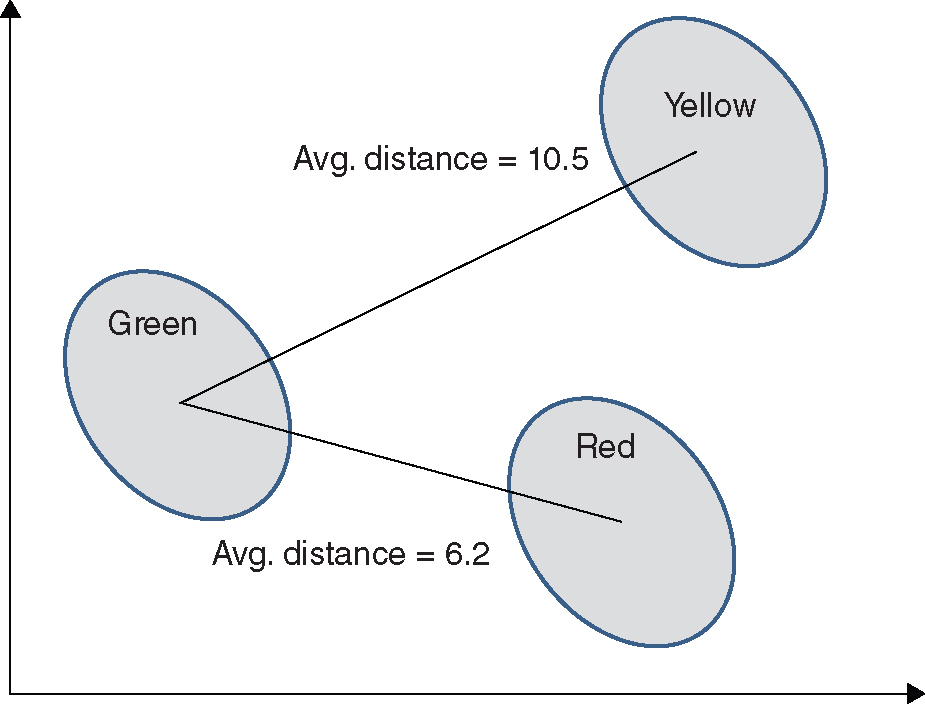
Figure 12.11 Validation of Scale—Distance between Green, Yellow, and Red Clients (with 49 variables)
After performing MTS optimization with an L64 OA, the results were as shown in Table 12.6.
After performing S/N ratio analysis and considering other practical constraints, 11 variables were selected as important. With these 11 variables, the performance of the scale was better than that of the scale with 49 variables in terms of separation. This is clear from Figure 12.12.

Figure 12.12 Separation between Clients (after Optimization, with 11 Variables)
Table 12.6 MTS Optimization with L64 Array

12.5.1 Improvements Made Based on Recommendations from MTS Analysis
A new measurement system was developed by including the 11 attributes from the following:
- Survey
- Volatility within the client
- Volatility within the company
The company was convinced that the performance of the measurement system with these 11 attributes was much more meaningful and objective as compared to traditional subjective evaluations.
12.6 Case Study: Understanding the Behavior Patterns of Defaulting Customers
This case study again concerns a financial institution. Following is a summary of this case.
This project is aimed at understanding the behavioral patterns of the customers that are or may be capable of defaulting on a particular loan. It was decided that a set of 10 variables would be used to explain such behavior patterns. The data from the customers who did not default was used to construct the reference group. After collecting data on default and nondefault customers, the MTS method was applied to construct and validate the scale with the Mahalanobis distance and correlation matrix. Table 12.7 shows the correlations between the 10 variables used in this study.
Figure 12.13 shows the separation between defaulting customers and the reference group. Based on this figure, we can say that the separation is very good, and we can validate the scale.
After conducting the optimization step, the number of variables was reduced to five (X4-X5-X7-X8-X9). With these variables, the separation was also quite good. Figure 12.14 shows the separation between the reference group and the defaulting customers optimization.
Table 12.7 Correlation Matrix
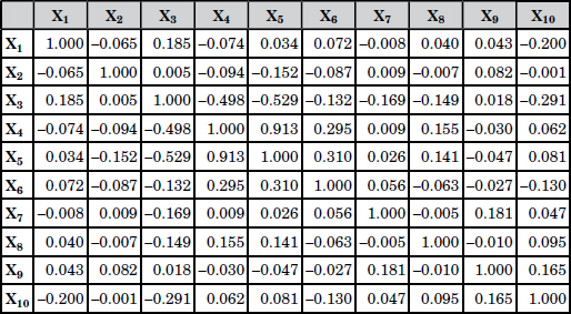
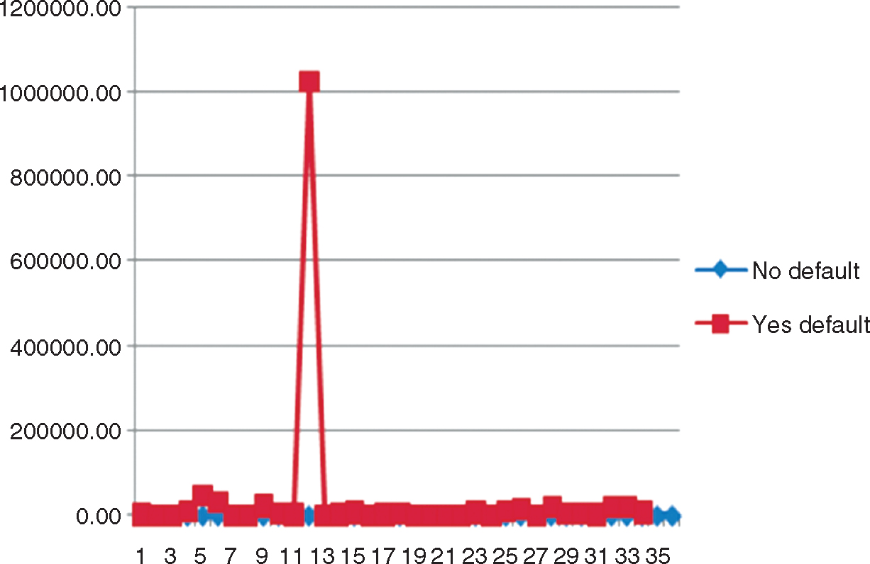
Figure 12.13 MTS Scale Validation
Since X4-X5-X7-X8-X9 are sufficient to distinguish the defaulting customers from the reference group, these variables were used to design strategies for preventing losses attributed to the defaulting customers.

Figure 12.14 Separation with Optimized Scale
12.7 Case Study: Marketing
This study involves an auto marketing application requiring that customers' buying patterns for different segments of the car market be identified. The objective of this study was to recognize the buying patterns of customers owning a particular model. It was decided that the behavior patterns would be explained using MTS analysis incorporating the following steps:
- Construct the reference group for a pattern under consideration (base pattern).
- Consider other patterns as abnormals (conditions outside the reference group).
- Select the useful variables by using orthogonal arrays and S/N ratios.
- Use the useful variables for future diagnosis.
- If there is prior knowledge about the abnormals, then recognize patterns by comparing them with the base pattern.
- Otherwise, repeat steps 1 through 4 for all other patterns and test the new observation against each to decide which pattern it belongs to.
In this case, the buying patterns were to be identified based on customer survey results. The variables considered for the survey were classified under the following categories:
- Personal views
- Purchase reasons
- Demographics
The customer survey data was obtained from a marketing-related database. After combining the variables in the three categories, 55 variables were considered, covering five car segments. As stated, the purpose of this case study was to identify the buying patterns of the five segments based on the 55 variables.
In some cases, the customers were asked to rank the variables on a scale from 1 to 4, where 1 meant strongly agree and 4 meant strongly disagree. After arranging the 55 variables in the desired order, they were denoted as X1, X2, . . . , X55 for the purpose of analysis. Since there were five segments and there was no prior knowledge about these patterns, MTS analysis was performed on all of the segments. For convenience, the five segments are denoted as S1, S2, . . . , S5.
12.7.1 Construction of the Reference Group
For each of the five segments, the reference group was built based on the data set. For example, the reference group for S1 was constructed by taking observations on 55 variables corresponding to that segment. With these reference groups, the corresponding MDs were calculated.
12.7.2 Validation of the Scale
The second stage in the MTS method is validation. The outside conditions for a given segment were chosen from the other segments. It was found that the abnormals, in all of the cases, had higher MDs; thus, the scale was validated.
12.7.3 Identification of Useful Variables
To identify a useful set from the 55 original variables, the L64(263) orthogonal array (OA) was chosen for each segment analysis. The S/N ratios were computed based on the larger-the-better criterion, because prior information about abnormals was not available.
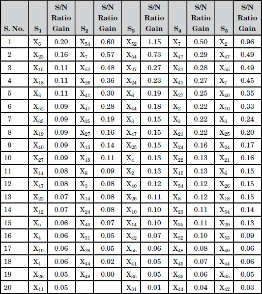
Table 12.8 provides the list of useful variables corresponding to all five segments. Since for each segment a suitable strategy was to be developed with a manageable number of variables, it was decided to restrict the number of variables per segment to 20. The selection of these variables was done based on the magnitude of gains in the S/N ratio.
With the useful set of variables, confirmation runs were conducted for all five segments. The results of the confirmation indicated that these variables were capable of recognizing the given patterns as effectively as in the case with all 55 variables. Figure 12.15 shows the recognition power of the useful variables in the respective car segments.
Decreasing the number of variables in the optimal system helped to reduce the complexity of the multidimensional systems and develop effective strategies to improve sales.
Table 12.8 Useful Variables Corresponding to the Five Segments
12.8 Case Study: Gear Motor Assembly
This case study was conducted at a document company. The purpose of life testing the 127K27330 gear-motor assembly was to measure all the parameters (or variables) and decide on the reusability of these motors. It is important to identify a suitable measure representing these parameters and based on which a decision on the reusability of a motor can be made. Since all of these parameters may not be necessary to make a decision, it is required that a useful set of parameters be identified to determine whether a used 127K27330 gear-motor assembly would be suitable for reuse. For convenience, the 127K27330 motor is simply referred to as the “motor” in the remainder of this section. This problem can be treated as a diagnosis problem, in which the reusability of a motor was decided based on the value of the Mahalanobis distance. Hence, the MTS method was applied to this problem.
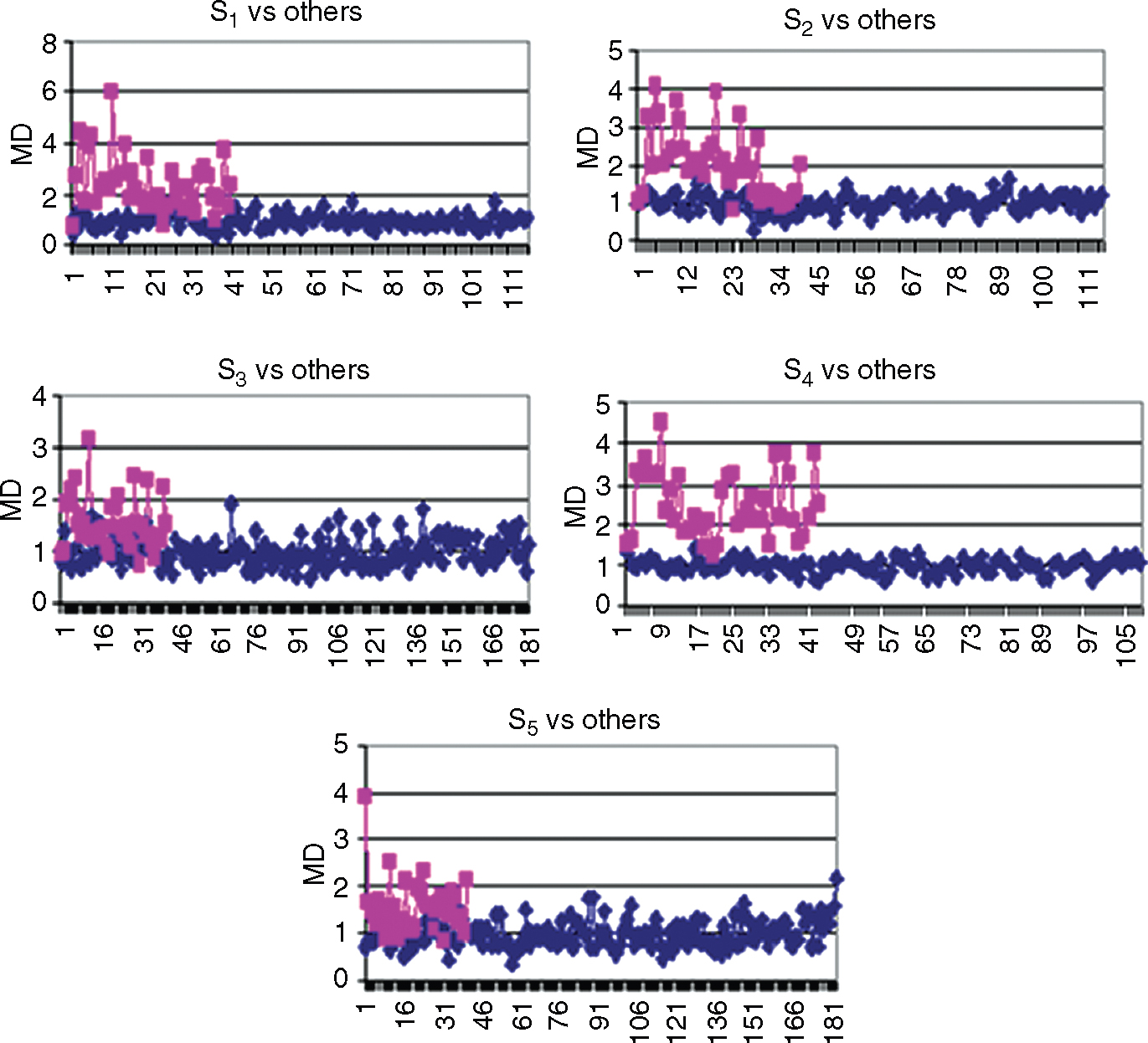
Figure 12.15 Pattern Recognition with a Useful Set of Variables
12.8.1 Apparatus
A diagram of the 127K27330 test fixture is shown in Figure 12.16. From left to right, the holding fixture consists of a hand shield, high-resolution encoder, hysteresis brake, customized brake coupling, the motor, and a Destaco clamp. The motor's output coupling engages the brake coupling, which turns the hysteresis brake, which turns the encoder. The Destaco clamp prevents any lateral movement.
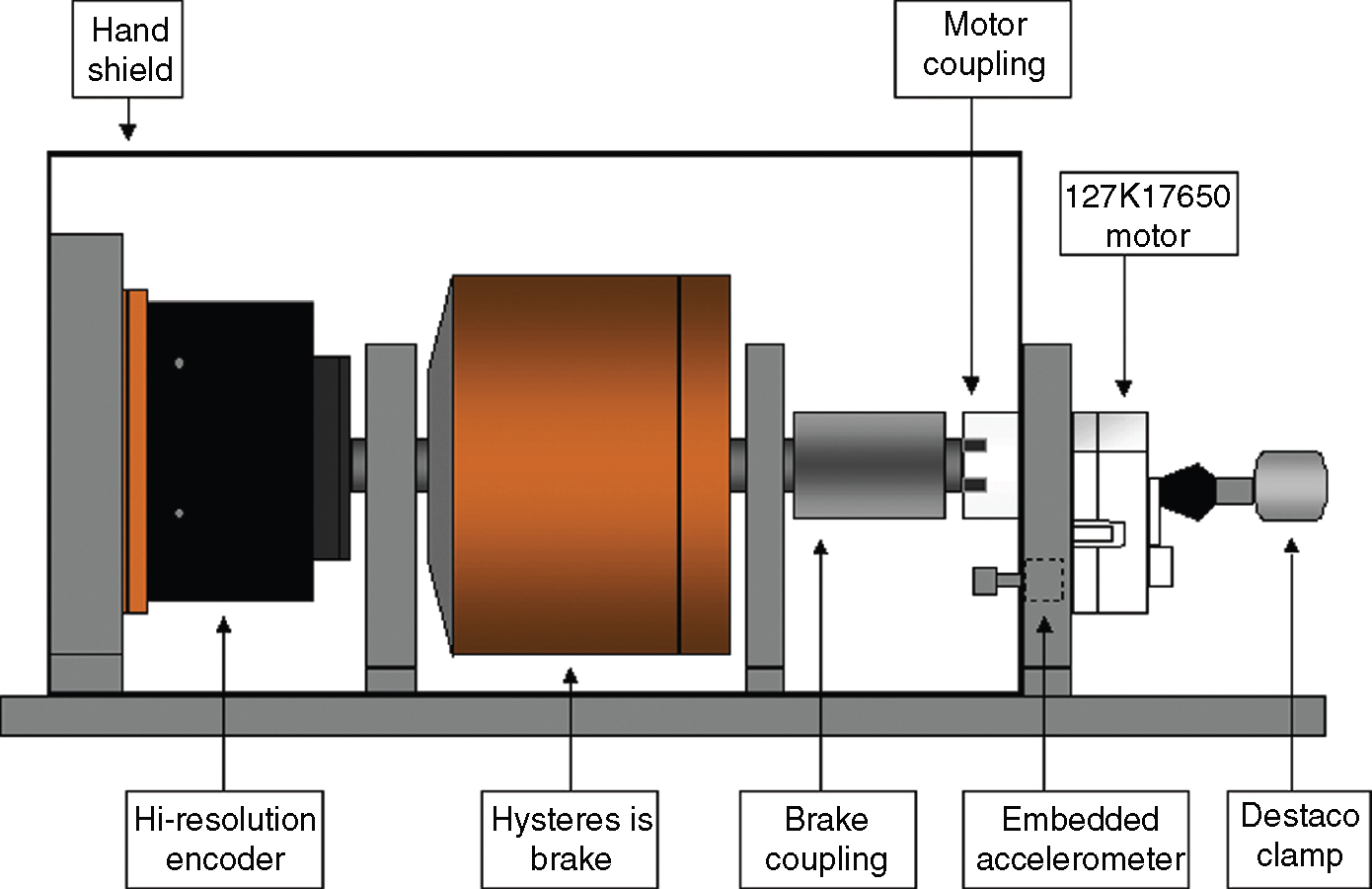
Figure 12.16 127K27330 Test Fixture
12.8.2 Sensors
A PCB accelerometer (Model J352A78, 100 mV/g) was used to measure vibration. This accelerometer was stud mounted in the motor mount plate (see Figure 12.16).A 1-ohm resistor was used for current sensing. A Gurley (Model 8435H, 32,000 pulses/revolution) high-resolution encoder was used to measure motion and speed.
12.8.3 High-Resolution Encoder
Because the speed of the motor is approximately 1.5 rpm, a standard tachometer could not be used, since its output voltage would be negligible. A high-resolution encoder from Gurley (Model 8435H) was used for measuring motor speed. This encoder has a resolution of 32,000 pulses/revolution. A US Digital PC6-84-4 quadrature interpolator was used to increase the resolution of this encoder from 32,000 to 128,000 pulses/revolution.
A LabView example program called Buffered Counting of Events.vi served as the basis for inputting and interpreting the encoder pulse stream.
If, for example, there is an incoming pulse train and it is required that the pulses be counted and the count value accumulated after every 5 milliseconds (ms), here is what needs to be done:
- Make one of the counters generate a pulse train of 5 ms (200 Hz) and connect the OUT of this counter (no. 1) to the GATE of the next counter (no. 2).
- Connect the signal to the SOURCE of counter 2.
- The pulse train generated by counter 1 goes high every 5 ms.
When it goes high for the first time, counter 2 starts counting the signal. It keeps counting until it sees another high at the gate, which would be after 5 ms. At this point, the count value of counter 2 is written to the buffer. Counter 2 is actually still counting. When it sees the next high on the gate, after 5 ms, again the counter value is written to the buffer. Therefore, the buffer would have monotonically increasing values representing the accumulated count of counter 1 after each 5-ms interval. We can do this buffered counting at any interval by changing the 200 Hz (5 ms) to some other value.
To summarize, the output of counter 1 is physically tied to the gate of counter 2. Counter 1 time-stamps the running count of counter 2.
12.8.4 Life Test
The life testing apparatus from the 127K1581 motor test was reused for the 127K27330 life test with a few modifications to the motor baseplate. A QuickBasic program called dc_motor.bas and an optomux/opto22 system provided electronic control. Ten new 127K27330 motors were used for the life test. The parameters were measured at intervals of 10,000 cycles starting from 0 cycles to 120,000 cycles during the life test.
12.8.5 Characterization
After every 10,000 cycles the 10 motors were taken off the test for characterization. The LabView characterization program is called hodaka_dc_motor.vi. The characterization program ran the motor at three different operating conditions: (1) motor voltage (mv) = 21.6 V, brake voltage (bv) = 4.95 V; (2) mv = 21.6 V, bv = 0 V; (3) mv = 12 V, bv = 4.95 V. These levels were specifically chosen to stress the motor and force a separation between new-motor performance and used-motor performance. The 4.95 V brake voltage corresponded to a 1.96-Nm (276.4-oz-in) load. In these tests, a personal computer, generic SA interface box, and National Instruments AT-MIO-16E-10 board were used for data acquisition.
Of the various parameters measured by hodaka_dc_motor.vi, the following parameters, in the three different operating conditions, were considered to be important:
- Current
- Vibration
- Speed
- Count—count measurements of counter 2
Some of the parameters could not be considered, because they were fixed while conducting the life test. Since speed measurements were derived from the counts by taking the derivative of the buffered counts, there was no need to consider both of them. Therefore, the parameter count was dropped from the analysis. We were left with nine variables: current (C), vibration (V), and speed (S) in three operating conditions. The variables were denoted as X1, X2, . . . , X9. The data on these parameters was collected by using hodaka_dc_motor.vi.
After collecting data on these nine variables, the MTS method was used for data analysis.
12.8.6 Construction of the Reference Group or Mahalanobis Space
Motors 1 through 10 were all new when life testing was started. The presumption was that all new motors are good. Therefore, the parameters measured at 0 cycles (corresponding to these motors) were used to construct the Mahalanobis space for the healthy group. When data about the motors was combined, there were numerous observations corresponding to the parameters at 0 cycles. These parameters reached steady state after some point in time. To verify this fact, data on these parameters was plotted on separate graphs. Figure 12.17 shows some of these graphs. From this figure, it is clear that that the parameters attained steady state after some point in time.
To construct the Mahalanobis space (MS), it was not necessary to consider all of the data because the number of observations in the data was large. Therefore, a subset of the original data was used for constructing the MS. The subset selection was done in such a way that it contained an equal number of observations from the steady state and from the transient state. This helped in constructing a uniform MS. Based on this, the MDs corresponding to the observations in the MS were calculated.
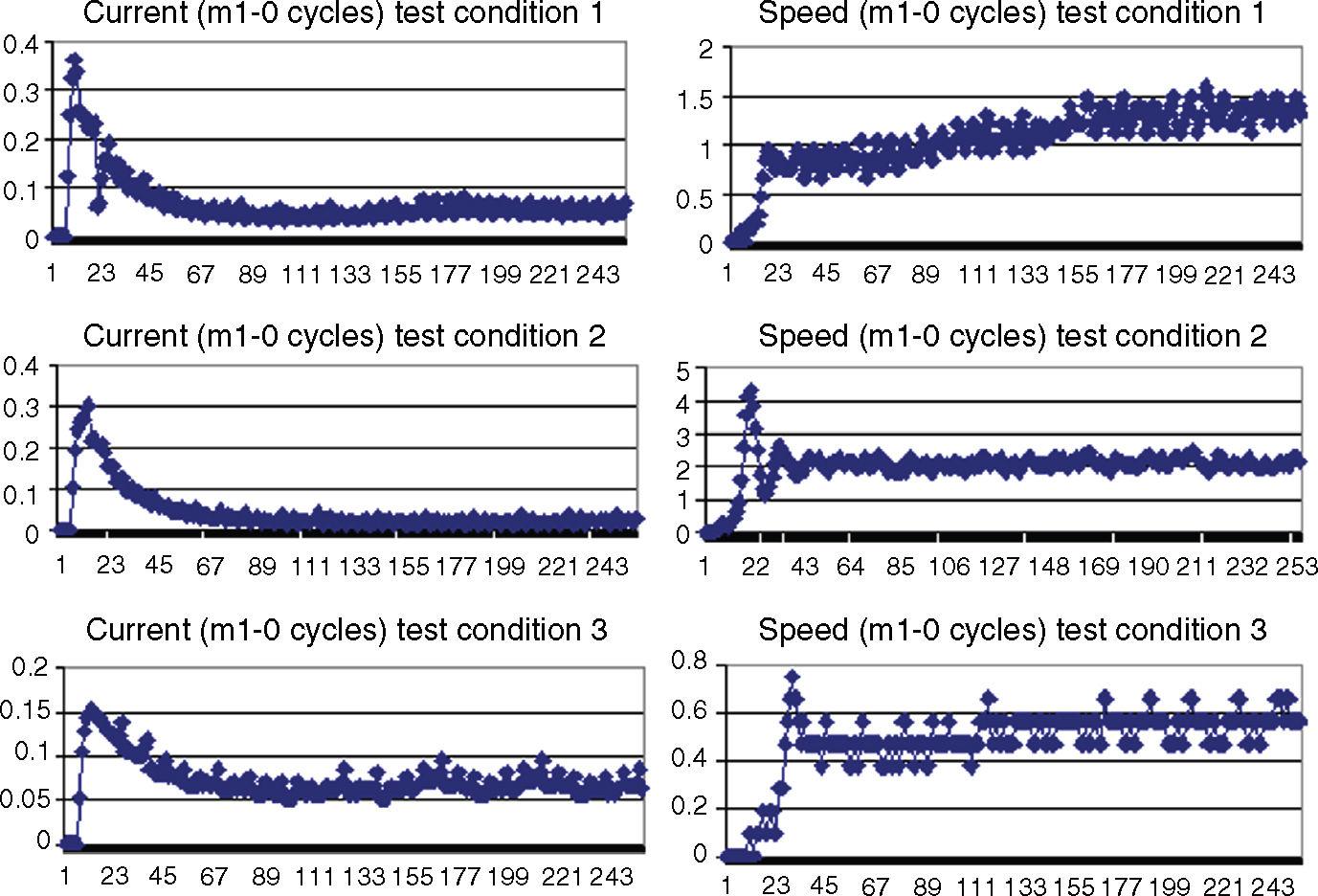
Figure 12.17 Patterns Corresponding to Some Parameters
12.8.7 Validation of the MTS Scale
After constructing the measurement scale, it was necessary to test the accuracy of the scale by measuring the MDs of some known conditions outside the MS. In this application, parameters measured after 10k, 20k . . . , 120k cycles were considered conditions outside the MS. Figure 12.18 shows the average MDs corresponding to these cycles. From this figure, we can say that the scale is good because abnormals have higher-value MDs. It is interesting to note that as the number of cycles increases the average MD also goes up, indicating that the motor performance deteriorates with an increase in the number of cycles.
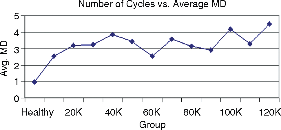
Figure 12.18 MTS Scale Validation
12.8.8 Selection of Useful Variables
In the third stage of the analysis, useful parameters were selected by using orthogonal arrays and S/N ratios. Since there were nine parameters, the L12(211) orthogonal array was used. Since we did not have prior knowledge about the abnormals, the larger-the-better type of S/N ratios was used in both methods. The results of MTS analysis are given in Table 12.9.
In Table 12.9, the variable combination X1-X2-X3-X5-X6-X8-X9 is considered as a useful combination because the variables in this combination have positive gains.
A confirmation run was conducted for the useful variables in both methods. It was found that from abnormal MDs we could distinguish normals and abnormals. Figure 12.19 shows the difference between the original combination and the optimal combination in terms of distinction between normals and abnormals. From this figure, it is clear that the distinction was much better with the optimal combination.
Table 12.9 S/N Ratio Average Responses and Gains (in dB units)
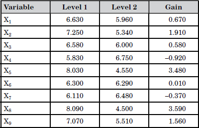
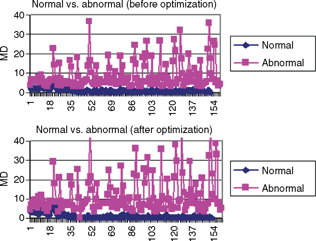
Figure 12.19 MTS Scale Performance Before and After Optimization
12.9 Conclusions
From this chapter, we can draw the following conclusions:
- After ensuring high-quality and reliable data, methods such as MTS are very useful in performing diagnostic analytics to derive important insights from the data.
- While doing analysis with multiple CDEs or variables, it is important to consider the correlation effects, since they affect overall information/data quality levels.
- Methods such as MTS are a great value adds to the analytical toolkit, and they can be easily modified to suit the big data context.
- Sometimes, it is important to identify the direction of abnormals in multivariate systems. With the help of the Gram-Schmidt process, we can determine the direction of the abnormalities, which enables a decision maker to take appropriate action. The S/N ratio can also be used as a strategic decision-making tool, since it can be effectively used to develop a good marketing/sales strategy for products in different regions.