
Chapter 8
Prospective Life Tables
Heather Booth
Australian National University
Canberra, Australia,
Rob J. Hyndman
Monash University
Melbourne, Australia,
Leonie Tickle
Macquarie University
Sydney, Australia,
8.1 Introduction
Prospective life tables depend on forecasting age-specific mortality. Considerable attention has been paid to methods for forecasting mortality in recent years. Much of this work has grown out of the seminal Lee-Carter method (Lee & Carter 1992). Other extrapolative approaches use Bayesian modelling, generalized linear modelling and state-space approaches. Methods for forecasting mortality have been extensively reviewed by Booth (2006) and Booth & Tickle (2008). This chapter covers various extrapolative methods for forecasting age-specific central death rates (also referred to as mortality rates). Also covered is the derivation of stochastic life expectancy forecasts based on mortality forecasts.
The main packages on CRAN for implementing life tables and mortality modelling are demography (see Hyndman 2012) and MortalitySmooth (see Camarda 2012), and we will concentrate on the methods implemented in those packages. However, mention is also made of other extrapolative approaches, and related R packages where these exist.
We will use, as a vehicle of illustration, U.S. mortality data. This can be extracted from the Human Mortality Database (2013) using the demography package.
> library(demography)
> usa <- hmd.mx("USA", "username", "password", "USA")
The username and password are for the Human Mortality Database.
The hmd.mx function downloads all available annual data by single years of age. Note that it is also possible to download data in 5-year age groups and that the methods described in this chapter can accommodate 5-year age groups. We use single years of age and annual years over time.
The object usa contains all the necessary data to forecast mortality:
> names(usa)
[1] "type" "label" "lambda" "year" "age" "pop" "rate"
A useful summary is given by
>usa
Mortality data for USA
Series: female male total
Years: 1933 - 2010
Ages: 0-110
usa is a 'demogdata' object of type 'mortality'. The functions in the demography package are designed to use demogdata objects.
In order to stabilize the high variance associated with high age-specific rates, it is necessary to transform the raw data by taking logarithms. Consequently, the mortality models considered in this chapter are all in log scale.
8.2 Smoothing Mortality Data
Suppose Dx,t is the number of deaths in calendar year t of people aged x,and Ecx,t is the total years of life lived between ages x,and x +1 in calendar year t, which can be approximated by the mid-year (central) population at age x in year t.
Mid-year populations can be obtained from the usa$pop list:
> names(usa$pop)
[1] "female" "male" "total"
For example, the matrix usa$pop$total contains the total population at age x (per row) at mid-year t (per column):
> usa$pop$total[1:5,1:6]
1933 1934 1935 1936 1937 1938
0 1963038 1920566 1940669 1953470 1967325 2012973
1 2034701 1927298 1896434 1924241 1945812 1965169
2 2178069 2106591 2037580 2020441 2063568 2102951
3 2229949 2191411 2126538 2056968 2040318 2086125
4 2274434 2226345 2187956 2122040 2053175 2038711
Similarly, the observed mortality rates, defined as
mx,t=Dx,t/Ecx,t'
are obtained from the list of matrices usa$rate. For example, rates for the total population are obtained by
> usa$rate$total[1:5,1:6]
1933 1934 1935 1936 1937 1938
0 0.061667 0.067866 0.061964 0.062786 0.061008 0.058018
1 0.009459 0.010622 0.008831 0.008895 0.008366 0.007793
2 0.004351 0.004852 0.004171 0.004199 0.004000 0.003563
3 0.003104 0.003230 0.002980 0.002870 0.002681 0.002463
4 0.002386 0.002451 0.002404 0.002272 0.002151 0.001912
Figure 8.1 shows mortality rates for U.S. males in 2003, based on the following R code:
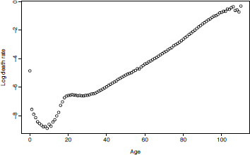
>plot(usa$age, log(usa$rate$male[,"2003"]), xlab= "Age", ylab="Log death rate")
Because usa is a 'demogdata' object, this graph can also be obtained by
>plot(usa, series="male", years=2003, type="p", pch=1)
This example shows that the mortality rates follow a smooth function with some observational error. The observational error has higher variance at very old ages (because the populations are small) and at childhood ages (because the mortality rates are low). (Note that observed mortality rates at very old ages can exceed 1 because the number of deaths at age x may exceed the mid-year population aged x.)
Thus, we observe {xi,mxi,t},t=1,...,n,i=1,...,p, , where
log mxi,t=ft(x∗i)+σt(x∗i)εt,i,
log denotes the natural logarithm, ft(x) is a smooth function of x,x∗i is the mid-point of age interval xi,n is the number of years and p is the number of ages in the observed data set, εt,i is an iid random variable and σt(x) allows the amount of noise to vary with x.
Then the observational variance, of σ2t(x), can be estimated assuming deaths are Poisson distributed (Brillinger 1986). Thus mx,t has approximate variance Dxt/(Ecx,t)2, , and the variance of log mx,t (via a Taylor approximation) is
σ2t(x)≈1/Dx,t.
Life tables constructed from the smoothed ft(x) data have lower variance than tables constructed from the original mt,x data, and thus provide better estimates of life expectancy. To estimate f, we can use a nonparametric smoothing method such as kernel smoothing, loess, or splines. Two smoothing methods for estimating ft(x) have been widely used, and both involve regression splines. We will briefly describe them here.
8.2.1 Weighted Constrained Penalized Regression Splines
Hyndman & Ullah (2007) proposed using constrained and weighted penalized regression splines for estimating ft(x) The weighting takes care of the heterogeneity due to σt(x) and a monotonic constraint for upper ages can lead to better estimates.
Following Hyndman & Booth (2008), we define weights proportional to the approximate inverse variances, wx,tαDx,t, , and use weighted penalized regression splines (Wood 2003, He & Ng 1999) to estimate the curve ft(x) in each year. Weighted penalized regression splines are preferred because they can be computed quickly and allow monotonicity constraints to be imposed relatively easily.
We apply a qualitative constraint to obtain better estimates of ft(x) especially when σt(x) is large. We assume that ft(x) is monotonically increasing for x>b for some b (say, b = 65 years). This monotonicity constraint allows us to avoid some of the noise in the estimated curves for high ages, and is not unreasonable for this application (after middle age, the older you are, the more likely you are to die). We use a modified version of the approach described in Wood (1994) to implement the monotonicity constraint.
Figure 8.2 shows the estimated smooth curve ft(x) for the U.S. male mortality data plotted in Figure 8.1. This is easily implemented in the demography package using the following code:
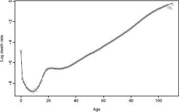
Smoothed male mortality rates for single years of age, United States 2003. The smooth curve, ft(x) , is estimated using weighted penalized regression splines with a monotonicity constraint for ages greater than 65.
smus <- smooth.demogdata(usa)
plot(usa, years=2003, series="male", type="p", pch=1, col="gray")
lines(smus, years=2003, series="male")
8.2.2 Two-Dimensional P-Splines
The above approach assumes ft(x) is a smooth function of x, but not of t. Hyndman & Ullah (2007) argued that the occurrence of wars and epidemics meant that !ft(x) should not be assumed to be smooth over time. In the absence of wars and epidemics, it is reasonable to assume smoothness in both the time and age dimensions. For this reason, we use data from 1950 in this subsection.
> usa1950 <- extract.years(usa, years=1950:2010)
Currie et al. (2004) proposed using two-dimensional splines. We will call this approach the Currie-Durban-Eilers or CDE method.
The CDE method adopts the generalized linear modelling (GLM) framework for the Poisson deaths Dx,t with two-dimensional P-splines. Here
Dx,t~P(Ecx,t.exp[s(x,t)])
where the number of deaths Dx,t will be proportional to the exposure, Ecx,t and ft(x)=exp[s(x,t)] will denote the mortality rate.
This is implemented in the MortalitySmooth package in R (Camarda 2012) and compared with the Hyndman & Ullah (2007) approach using the following code:
> library(MortalitySmooth)
> Ext <- usa1950$pop$male
> Dxt <- usa1950$rate$male * Ext
> fitBIC <- Mort2Dsmooth(x=usa1950$age, y=usa1950$year, Z=Dxt, offset=log(Ext))
> par(mfrow=c(1,2))
> plot(fitBIC$x, log(usa1950$rate$male[,"2003"]), xlab="Age", ylab="Log death rate",
+ main="USA: male death rates 2003", col="gray")
> lines(fitBIC$x, log(fitBIC$fitted.values[,"2003"]/Ext[,"2003"]))
> lines(smus,year=2003, series="male", lty=2)
> legend("topleft",lty=1:2, legend=c("CDE smoothing", "HU smoothing"))
> plot(fitBIC$y, log(Dxt["65",]/Ext["65",]), xlab="Year", ylab="Log death rate",
+ main="USA: male death rates age 65", col="gray")
> lines(fitBIC$y, log(fitBIC$fitted.values["65",]/Ext["65",]))
> lines(smus$year, log(smus$rate$male["65",]), lty=2)
> legend("bottomleft", lty=1:2, legend=c("CDE smoothing", "HU smoothing"))
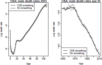
Figure 8.3 shows the estimated smooth curve, ft(x) , for the U.S. male mortality data using the bivariate P-spline (CDE) method (Currie et al. 2004) and the univariate penalized regression spline method of Hyndman & Ullah (2007). Note that the univariate method is not smooth in the time dimension (right panel), but gives a better estimate for the oldest ages due to the monotonic constraint.
> par(mfrow=c(1,2))
> year=usa1950$year[seq(1,62,by=3)]
> age=usa1950$age[seq(1,111,by=3)]
> persp(age, year, log(usa1950$rate$male[seq(1,111,by=3), seq(1,62,by=3)]), theta=-30,
+ main="Observed death rates", col=grey(.93), shade=TRUE, xlab="Age", ylab="",
+ zlab="Log death rate", ticktype="detailed",cex.axis=0.6, cex.lab=0.6)
> persp(age, year, predict(fitBIC)[seq(1,111,by=3),seq(1,62,by=3)], theta=-30,
+ main="Smoothed death rates", col=grey(.93), shade=TRUE, xlab="Age", ylab="",
+ zlab="Log death rate", ticktype="detailed", cex.axis=0.6, cex.lab=0.6)
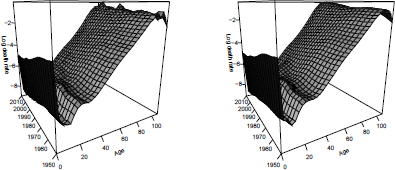
Figure 8.4 shows smoothing of the 1950-2010 dataset. On the left are observed death rates mt,x and on the right are the estimated smoothed rates, ft(x)
8.3 Lee—Carter and Related Forecasting Methods
The Lee-Carter (LC) method introduced in Lee & Carter (1992) for forecasting mortality rates uses principal components analysis to decompose the age-time matrix of log central death rates into a linear combination of age and time parameters. The time parameter is used in forecasting.
LC has spawned numerous variants and extensions. The two main variants of LC are Lee-Miller (LM) (Lee & Miller 2001) and Booth-Maindonald-Smith (BMS) (Booth et al. 2002). Others result from different combinations of possible options. These variants are collectively referred to as “LC methods” . A major extension of this approach uses functional data models (FDM); first proposed by Hyndman & Ullah (2007), it was further developed by Hyndman & Booth (2008) and Hyndman & Shang (2009). Again, various combinations of options produce variations within the collectively labeled “HU methods” .
We identify six methods by their proponents; these are listed in Table 8.1 where the defining features of the models are shown. Most authors referring to the “Lee-Carter method” actually refer to the generic model in which all available data are used, there is no adjustment of the time parameter prior to forecasting, and fitted rates are used as jump-off rates; Booth et al. (2006) labeled this “LCnone” . Note that within the options listed in Table 8.1 there are twenty-four possible combinations (4 adjustment options × 3 data period options × 2 jump-off options) for the LC methods. For the HU methods, additional options have been defined by varying the data period option to include 1950 (Shang et al. 2011). Clearly, any date can be used for the start of the data period.
Lee-Carter and Hyndman-Ullah methods by defining features.
Method |
Data Period |
Smoothing |
Adjustment to Match |
Jump-off Rates |
Reference |
Lee-Carter Methods |
|||||
LC |
All |
No |
Dt |
Fitted |
Lee & Carter (1992) |
LM |
1950 |
No |
e(0) |
Observed |
Lee & Miller (2001) |
BMS |
Linear |
No |
Dx,t |
Fitted |
Booth et al. (2002) |
LCnone |
All |
No |
- |
Fitted |
- |
Hyndman-Ullah Methods |
|||||
HU |
- |
Yes |
- |
Fitted |
Hyndman & Ullah (2007) |
HUrob |
- |
Yes |
- |
Fitted |
Hyndman & Ullah (2007) |
HUw |
- |
Yes |
- |
Fitted |
Hyndman & Shang (2009) |
In this section, we begin with the complete available dataset usa, for which ages range from 0 to 110+ and years range from 1933 to 2010.
> usa
Mortality data for USA
Series: female male total
Years: 1933 - 2010
Ages: 0-110
Appropriate age ranges and fitting periods are defined for each method.
As the Lee-Carter methods do not incorporate smoothing, it is advisable to avoid erroneous rates at the oldest ages when using these methods.
> usa.90 <- extract.ages(usa, ages=0:90)
In this example, the upper age group is then 90+.
8.3.1 Lee—Carter (LC) Method
The model structure proposed by Lee & Carter (1992) is given by
log(mx,t)=ax+bxkt+εx,t,(8.1)
where ax is the age pattern of the log mortality rates averaged across years, bx is the first principal component reflecting relative change in the log mortality rate at each age, kt is the first set of principal component scores by year t and measures the general level of the log mortality rates, and εx,t is the residual at age x and year t. The model assumes homoskedastic error and is estimated using a singular value decomposition.
The LC model in Equation (8.1) is over-parameterized in the sense that the model structure is invariant under the following transformations:
{ax,bx,kt}↦{ax,bx/c,ckt},
{ax,bx,kt}↦{ax−cbx,bx,kt+c}.
In order to ensure the model's identifiability, Lee & Carter (1992) imposed two constraints, given as
∑nt=1kt=0, ∑xpx=x1bx=1.
In addition, the LC method adjusts kt by refitting to the total number of deaths. This adjustment gives more weight to high rates, thus roughly counterbalancing the effect of using a log transformation of the mortality rates. The adjusted kt is then extrapolated using ARIMA models. Lee & Carter (1992) used a random walk with drift (RWD) model, which can be expressed as
kt=kt−1+d+et,
where d is known as the drift parameter and measures the average annual change in the series, and et is an uncorrelated error. It is notable that the RWD model provides satisfactory results in many cases (Tuljapurkar, Li & Boe 2000, Lee & Miller 2001, Lazar & Denuit 2009). From this forecast of the principal component scores, the forecast age-specific log mortality rates are obtained using the estimated age effects ax and bx , and setting εx,t=0 , in Equation (8.1).
The LC method is implemented in the R demography package as follows:
> lc.male <- lca(usa.90, series="male")
> forecast.lc.male <- forecast(lc.male, h=20)
The estimated age parameters ax and bx, and the estimated time parameter kt are respectively obtained using lc.male$ax, lc.male$bx and lc.male$kt. Similarly, the forecast time parameter (rescaled to zero in the jump-off year 2010) is obtained using forecast.lc.male$kt.
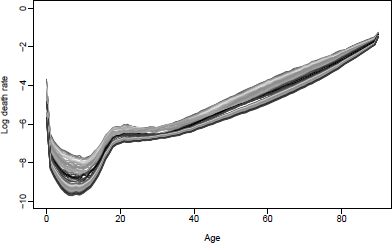
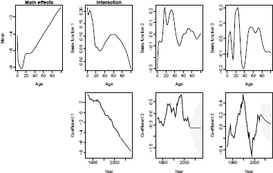
The data (Figure 8.5), model parameters (Figure 8.6) and forecasts can be viewed via
> plot(usa.90, series="male")
> plot(lc.male)
> plot(forecast.lc.male, plot.type="component")
> plot(usa.90, series="male", ylim=c(-10,0), lty=2)
> lines(forecast.lc.male)
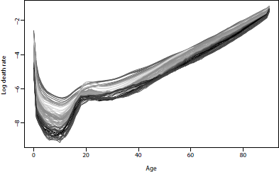
U.S. male mortality rates, 1933-2010. Note the emergence of the “accident hump” at about age 20 and the effect of deaths due to AIDS at about ages 25-44 in 1985-1995.
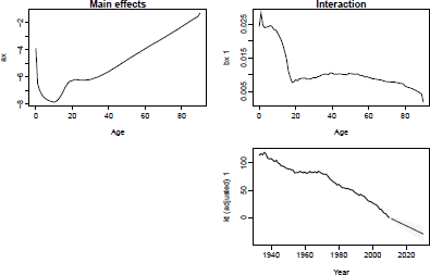
LC model and forecast, U.S. male mortality. Fitting period = 1933-2010; forecasting horizon = 20 years.
The LC method without adjustment of kt (LCnone) is achieved by choosing the adjustment option adjust="none".
> lcnone.male <- lca(usa.90, series="male", adjust="none")
The effect of the LC adjustment of kt is seen in Figure 8.7 via
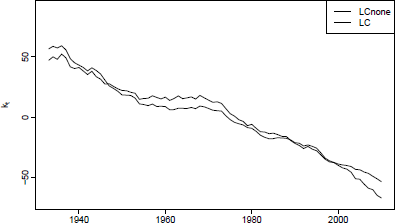
> plot(lcnone.male$kt, ylab="kt",ylim=c(-70,90), xlab="")
> lines(lc.male$kt, lty=2)
> legend("topright", lty=1:2, legend=c("LCnone","LC"))
Differences between these two lines in the first and last years of the fitting period can have a substantial effect on the forecast.
An alternative, and more efficient, approach to estimating a Lee-Carter model was described by Brouhns et al. (2002); it involves embedding the method in a Poisson regression model, and using maximum likelihood estimation. This can be achieved in R using, for example,
> lca(usa, series="male", adjust="dxt")
8.3.2 Lee—Miller (LM) Method
The LM method is a variant of the LC method. It differs from the LC method in three ways:
- The fitting period begins in 1950;
- The adjustment of kt
- involves fitting to the life expectancy e(0) in year t;
- The jump-off rates are the observed rates in the jump-off year instead of the fitted rates.
In their evaluation of the LC method, Lee & Miller (2001) found that the pattern of change in mortality rates was not constant over time, which is a strong assumption of the LC method. Consequently, the adjustment of historical principal component scores resulted in a large estimation error. To overcome this, Lee & Miller (2001) adopted 1950 as the commencing year of the fitting period due to different age patterns of change for 1900-1949 and 1950-1995. This fitting period had previously been used by Tuljapurkar et al. (2000).
In addition, the adjustment of kt was done by fitting to observed life expectancy in year t, rather than by fitting to total deaths in year t. This has the advantage of eliminating the need for population data. Further, Lee & Miller (2001) found a mismatch between fitted rates for the final year of the fitting period and observed rates in that year. This jump-off error was eliminated by using observed rates in the jump-off year.
The LM method is implemented as follows:
> lm.male <- lca(usa.90, series="male", adjust="e0", years=1950:max(usa$year))
> forecast.lm.male <- forecast(lm.male, h=20, jumpchoice = "actual")
The LM method has been found to produce more accurate forecasts than the original LC method (Booth et al. 2005, 2006).
8.3.3 Booth—Maindonald—Smith (BMS) Method
The BMS method is another variant of the LC method. The BMS method differs from the LC method in three ways:
- The fitting period is determined on the basis of a statistical ‘goodness of fit' criterion, under the assumption that the principal component score k1 is linear;
- The adjustment of Kt involves fitting to the age distribution of deaths rather than to the total number of deaths;
- The jump-off rates are the fitted rates under this fitting regime.
A common feature of the LC method is the linearity of the best fitting time series model of the first principal component score, but Booth, Maindonald & Smith (2002) found the linear time series to be compromised by structural change. By first assuming the linearity of the first principal component score, the BMS method seeks to achieve the optimal ‘goodness of fit' by selecting the optimal fitting period from all possible fitting periods ending in year n. The optimal fitting period is determined based on the smallest ratio of the mean deviances of the fit of the underlying LC model to the overall linear fit.
Instead of fitting to the total number of deaths, the BMS method uses a quasi-maximum likelihood approach by fitting the Poisson distribution to model age-specific deaths, and using deviance statistics to measure the ‘goodness of fit' (Booth, Maindonald & Smith 2002). The jump-off rates are taken to be the fitted rates under this adjustment.
The BMS method is implemented thus:
> bms.male <- bms(usa.90 series="male", minperiod = 30, breakmethod = "bms")
> forecast.bms.male <- forecast(bms.male, h=20)
It is advisable to review the deviances (Figure 8.8) and the automatically chosen fitting period, which is based on a local minimum of the ratio of total to base mean deviances.
> plot(bms.male$mdevs, main="Mean deviances for base and total models", xlab="")
> bms.male$year[1]
[1] 1967
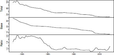
Mean deviances for base and total models and their ratio, U.S. male mortality, 1933-2010.
Estimated kt and forecast rates (Figure 8.9) are obtained via
> plot(bms.male$kt)
> plot(usa.90, series="male", years=bms.male$year[1]:max(usa$year),
+ ylim=c(-10,0), lty=2, main="BMS method: observed (1979-2010)
and forecast (2011-2030) rates")
> lines(forecast.bms.male)
Observed (1979-2010) and forecast (2011-2030) mortality rates using the BMS method for U.S. males.
An alternative implementation using the lca() function, which permits all possible variants to be produced, is:
> bms.male <- lca(usa.90, series="male", adjust="dxt", chooseperiod=TRUE,
+ minperiod = 30, breakmethod = "bms")
> forecast.bms.male <- forecast(bms.male, h=20)
Forecasts from the BMS method have been found to be more accurate than those from the original LC method and of similar accuracy as those from the LM method (Booth et al. 2005, 2006).
8.3.4 Hyndman—Ullah (HU) Method
Using the functional data analysis paradigm of Ramsay & Silverman (2005), Hyndman & Ullah (2007) proposed a nonparametric method for modeling and forecasting log mortality rates. This approach extends the LC method in four ways:
- The log mortality rates are smoothed prior to modeling;
- Functional principal components analysis is used;
- More than one principal component is used in forecasting;
- The forecasting models for the principal component scores are typically more complex than the RWD model.
The log mortality rates are smoothed using penalized regression splines as described in Section 8.2. To emphasize that age, x, is now considered a continuous variable, we write mt(x) to represent mortality rates for age x∈[x1,xp] in year t. We then define zt(x)= logmt(x) and write
zt(xi)=ft(xi)+σt(xi)εt,i,, i=1,...,p, t=1,...,n,(8.2)
where ft(xi) denotes a smooth function of x as before; σt(xi) allows the amount of noise to vary with xi in year t, thus rectifying the assumption of homoskedastic error in the LC model; and εt,i is an independent and identically distributed standard normal random variable.
Given continuous age x, functional principal components analysis (FPCA) is used in the decomposition. The set of age-specific mortality curves is decomposed into orthogonal functional principal components and their uncorrelated principal component scores. That is,
ft(x)=a(x)+∑Jj=1bj(x)k(x)kt,j+et(x),(8.3)
where a(x) is the mean function estimated by ˆa(x)=1n∑nt=1ft(x);{b1(x),...bJ(x)} is a set of the first J functional principal components; {kt,1,...,kt,J} is a set of uncorrelated principal component scores; et(x) is the residual function with mean zero; and J<n is the number of principal components used. Note that we use a(x) rather than ax to emphasise that x is not treated as a continuous variable.
Multiple principal components are used because the additional components capture nonrandom patterns that are not explained by the first principal component (Booth, Maindon- ald & Smith 2002, Renshaw & Haberman 2003, Koissi, Shapiro & Hognas 2006). Hyndman & Ullah (2007) found J=6 to be larger than the number of components actually required to produce white noise residuals, and this is the default value. The conditions for the existence and uniqueness of kt,j are discussed by Cardot, Ferraty & Sarda (2003).
Although Lee & Carter (1992) did not rule out the possibility of a more complex time series model for the kt series, in practice an RWD model has typically been employed in the LC method. For higher order principal components, which are orthogonal by definition to the first component, other time series models arise for the principal component scores. For all components, the HU method selects the optimal time series model using standard model-selection procedures (e.g. AIC). By conditioning on the observed data I={z1(x),...,zn(x)} and the set of functional principal components B={b1(x),...,bJ(x)}, , the h-step-ahead forecast of zn+h(x) can be obtained by
ˆzn+h|n(x)=Ε[zn+h(x)|I,B]=ˆa(x)+∑Jj=1bj(x)ˆkn+h|n,j,
where ˆkn+h|n,j denotes the h-step-ahead forecast of kn+h,j using a univariate time series model, such as the optimal ARIMA model selected by the automatic algorithm of Hyndman & Khandakar (2008), or an exponential smoothing state space model (Hyndman et al. 2008). Because of the orthogonality of all components, it is easy to derive the forecast variance as
ˆυn+h|n(x)=var[zn+h(x)|I,B]=σ2a(x)+∑Jj=1b2j(x)un+h|n,j+υ(x)+σat(x),
where σ2a is the variance of !ˆa(x);un+h,n,j is the variance of ! kn+h,j|k1,j,...,kn,j (obtained from the time series model); ! υ(x) is the variance of ! et(x) and σt(x) is defined in (8.2). This expression is used to construct prediction intervals for future mortality rates in R.
For the Hyndman-Ullah methods, we return to the complete dataset usa.
> usa
Mortality data for USA
Series: female male total
Years: 1933 - 2010
Ages: 0-110
In order to avoid the war years, the fitting period commences in 1950. Given that smoothing is employed, the age range is 0 to 100+.
> usa1950.100 <- extract.years(extract.ages(usa, 0:100), years=1950:max(usa$year))
> usa1950.100
Mortality data for USA
Series: female male total
Years: 1950 - 2010
Ages: 0 - 100
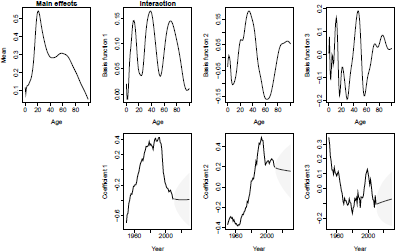
The HU method is implemented as below. The model and forecast are seen in Figures 8.10 and 8.11.
> smus1950.100 <- smooth.demogdata(usa1950.100)
> fdm.male <- fdm(smus1950.100, series="male", order=3)
> forecast.fdm.male <- forecast.fdm(fdm.male, h=20)
> plot(forecast.fdm.male, plot.type="component")
> plot(smus1950.100, series="male", ylim=c(-10,0), lty=2, main ="HU method:
+ observed (1950-2010) and forecast (2011-2030) rates")
> lines(forecast.fdm.male)
HU model and forecast, U.S. male mortality. Fitting period = 1950-2010; forecasting horizon = 20 years.
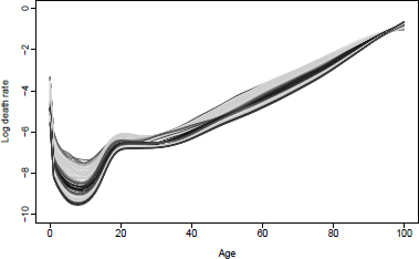
Observed (1950-2000) and forecast (2011-2030) mortality rates using the HU method for U.S. males.
8.3.5 Robust Hyndman-Ullah (HUrob) Method
The presence of outliers can seriously affect the performance of modelling and forecasting. The HUrob method is designed to eliminate their effect. This method utilizes the reflection- based principal component analysis (RAPCA) algorithm of Hubert, Rousseeuw & Verboven (2002) to obtain projection-pursuit estimates of principal components and their associated scores. The integrated squared error provides a measure of the accuracy of the principal component approximation for each year (Hyndman & Ullah 2007). Outlying years would result in a larger integrated squared error than the critical value obtained by assuming normality of et(x) (see Hyndman & Ullah 2007, for details). By assigning zero weight to outliers, the HU method can then be used to model and forecast mortality rates without the possible influence of outliers.
The HUrob method is implemented as follows:
> fdm.male <- fdm(smus1950.100, series="male", method="rapca")
> forecast.fdm.male <- forecast.fdm(fdm.male, h=20)
> plot(smus1950.100, series="male", ylim=c(-10,0), lty=2, main ="HUrob method:
+ observed (1950-2010) and forecast (2011-2030) rates")
> lines(forecast.fdm.male)
8.3.6 Weighted Hyndman-Ullah (HUw) Method
The HU method does not weight annual mortality curves in the functional principal components analysis. However, it might be argued that more recent experience has greater relevance to the future than more distant experience. The HUw method uses geometrically decaying weights in the estimation of the functional principal components, thus allowing these quantities to be based more on recent data than on data from the distant past.
The weighted functional mean a∗(x) is estimated by the weighted average
ˆa∗(x)=∑nt=1wtft(x),(8.4)
where {wt=β(1−β)n−t,t=1,...,n} denotes a set of weights, and 0<β<1 1denotes the weight parameter. Hyndman & Shang (2009) describe how to estimateβ fl from the data.
The set of weighted curves {wt[ft(x)−ˆa∗(x)];t=1,...,n} is decomposed using FPCA:
ft(x)=ˆa∗(x)+∑Jj=1b∗j(x)kt,j+et(x),(8.5)
where {b∗1(x),...,b∗J(x)} is a set of weighted functional principal components. By conditioning on the observed data I={z1(x),...,zn(x)} and the set of weighted functional principal components B∗ , the h-step-ahead forecast of zn+h(x) can be obtained by
ˆzn+h|n(x)=Ε[zn+h(x)|I,B∗]=ˆa∗(x)+∑Jj=1b∗j(x)ˆkn+h|n,j.
The HUw method is implemented as follows:
> fdm.male <- fdm(smus1950.100, series="male", method="classical", weight=TRUE, beta=0.1)
> forecast.fdm.male <- forecast.fdm(fdm.male, h=20)
> plot(smus1950.100, series="male", ylim=c(-10,0), lty=2, main = "HUw method:
+ observed (1950-2010) and forecast (2011-2030) rates")
lines(forecast.fdm.male)
8.4 Other Mortality Forecasting Methods
Other extrapolative mortality forecasting methods are included here for completeness, but are not considered in detail as the methods are not fully implemented in packages available on CRAN.
A number of methods have been developed to account for the significant impact of cohort (year of birth) in some countries. In the United Kingdom, males born around 1931 have experienced higher rates of mortality improvement than earlier or later cohorts (Willets 2004); less marked effects have also been observed elsewhere (Cairns 2009).
The Renshaw and Haberman (RH) (2006) extension to Lee-Carter to include cohort effects can be written as1
log(mx,t)=ax+b1xkt+b2xγt−x+εx,t,(8.6)
where ax is the age pattern of the log mortality rates averaged across years kt represents the general level of mortality in year t,γt−x represents the general level of mortality for the cohort born in year (t−x),b1x and b2x measure the relative response at age x to changes in kt and γt−x , respectively, and εx,t is the residual at age x. The fitted kt t and γt−x parameters are forecast using univariate time series models. The model can be implemented using the ilc functions (Butt & Haberman 2009).
A subsequent related model in which b2x is set equal to 1 at all ages (Haberman & Renshaw 2011) was found to resolve some forecasting issues associated with the original. The Age-Period-Cohort (APC) model (Currie 2006) incorporates age, time and cohort effects that are independent in their effects on mortality,
log(mx,t)=ax+kt+γt−x+εx,t.(8.7)
The two-dimensional P-spline method of Currie et al. (2004) has already been described in Section 8.2. Forecast rates are estimated simultaneously with fitting the mortality surface. Implementation of the two-dimensional P-spline method to produce mortality forecasts uses the MortalitySmooth package. Forecasts of U.S. male mortality rates and plots of age 65 and age 85 forecast rates with prediction intervals can be produced as follows, following the commands already shown in Section 8.2:
> library(MortalitySmooth)
> forecastyears <- 2011:2030
> forecastdata <- list(x=usa1950$age, y=forecastyears)
> CDEpredict <- predict(fitBIC, newdata=forecastdata, se.fit=TRUE)
> whiA <- c(66,86)
> plot(usa1950, series="male", age=whiA-1, plot.type="time",
+ xlim=c(1950,2030), ylim=c(-6.2,-1), xlab="years",
+ main="USA: male projected death rates using 2-dimensional CDE method", col=c(1,2))
> matlines(forecastyears, t(CDEpredict$fit[whiA,]), lty=1, lwd=2)
> matlines(forecastyears, t(CDEpredict$fit[whiA,]+2*CDEpredict$se.fit[whiA,]), lty=2)
> matlines(forecastyears, t(CDEpredict$fit[whiA,]-2*CDEpredict$se.fit[whiA,]), lty=2)
> legend("bottomleft", lty=1, col=1:2, legend=c("Age 65", "Age 85"))
In addition to being applied in the age and period dimensions, the two-dimensional P-spline method can incorporate cohort effects by instead being applied to age-cohort data.
Cairns et al. (2006a) have forecast mortality at older ages using a number of models for logit (qx,t)=log[qx,t/(1−qx,t)], , where qx,t is the probability that an individual aged x at time t will die before time t+1. . The original CBD model (Cairns et al. 2006a) is
logit(qx,t)=k1t+(x−ˉx)k2t+εx,t,(8.8)
where ˉx is the mean age in the sample range. Later models (Cairns 2009) incorporate a combination of cohort effects and a quadratic term for age:
logit(qx,t)=k1t+(x−ˉx)k2t+γt−x+εx,t,(8.9)
logit(qx,t)=k1t+(x−ˉx)k2t+((x−ˉx)2−ˆσ2x)+γt−x+εx,t,(8.10)
logit(qx,t)=k1t+(x−ˉx)k2t+(xc−x)γt−x+εx,t,(8.11)
where the constant parameter xc is to be estimated and the constant ˆσ2x is the mean of (x−ˉx)2 Other authors (e.g., Plat 2009) have proposed related models.
The LifeMetrics R software package implements the Lee-Carter method (using maximum likelihood estimation and a Poisson distribution for deaths) along with RH, APC, P-splines and the four CBD methods. The software, which is not part of CRAN, is available from www.jpmorgan.com/pages/jpmorgan/investbk/solutions/lifemetrics/software. The software and the methods it implements is described in detail in Coughlan et al. (2007).
De Jong & Tickle (2006) (DJT) tailor the state space framework to create a method that integrates model estimation and forecasting, while using B-splines to reduce dimensionality and build in the expected smooth behaviour of mortality over age. Compared with Lee-Carter, the method uses fewer parameters, produces smooth forecast rates and offers the advantages of integrated estimation and forecasting. A multi-country evaluation of out-of-sample forecast performance found that LM, BMS, HU and DJT gave significantly more accurate forecast log mortality rates relative to the original LC, with no one method significantly more accurate than the others (Booth et al. 2006).
8.5 Coherent Mortality Forecasting
In modelling mortality for two or more sub-populations of a larger population simultaneously, it is usually desirable that the forecasts are non-divergent or “coherent” . The Product-Ratio method (Hyndman et al. 2013) achieves coherence through the convergence to a set of appropriate constants of forecast age-specific ratios of death rates for any two sub-populations. The method makes use of functional forecasting (HU methods).
The method is presented here in terms of forecasting male and female age-specific death rates; extension to more than two sub-populations is straightforward (Hyndman et al. 2013). Let st,F(x)=exp[ft,F(x)] denote the smoothed female death rate for age x and year t=1,...,n. Similar notation applies for males.
Let the square roots of the products and ratios of the smoothed rates for each sex be
pt(x)=√st,M(x)st,F(x) and rt(x)=√st,M(x)/st,F(x).
These are modeled by functional time series models:
log[pt(x)]=μp(x)+∑Kk=1βt,kϕk(x)+et(x),(8.12a)
log[rt(x)]=μr(x)+∑Lℓ=1γt,ℓψℓ(x)+wt(x),(8.21b)
where the functions {ϕk(x)} and {ψℓ(x)} are the principal components obtained from decomposing .{pt(x)} and {rt(x)}, , respectively, and βt,k and γt,ℓ are the corresponding principal component scores. The function μp(x) is the mean of the set of curves {pt(x)}, , and µr(x) is the mean of {rt(x)}. The error terms, given by et(x) and wt(x) , have zero mean and are serially uncorrelated.
The coefficients {βt,1,...,βt,K} and {γt,1,...,γt,L} are forecast using time series models, as detailed in Section 8.3.4. To ensure the forecasts are coherent, the coefficients {γt,ℓ} are constrained to be stationary processes. The forecast coefficients are then multiplied by the basis functions, resulting in forecasts of the curves pt(x) and rt(x) for future t. If pn+h|n(x) and rn+h|n(x) are h-step forecasts of the product and ratio functions, respectively, then forecasts of the sex-specific death rates are obtained using sn+h|n,M(x)=pn+h|n(x)rn+h|n(x) and sn+h|n,F(x)=pn+h|n(x)/rn+h|n(x). The method makes use of the fact that the product and ratio behave roughly independently of each other provided the sub-populations have approximately equal variances. (If there are substantial differences in the variances, the forecasts remain unbiased but less efficient.)
The Product-Ratio method is illustrated in Figure 8.12, Figure 8.13 and Figure 8.14 and implemented as follows:
> usa.pr <- coherentfdm(smus1950.100, weight=TRUE, beta=0.05)
> usa.pr.f <- forecast(usa.pr, h=20)
> plot(usa.pr.f$product, plot.type="component", components=3)
> plot(usa.pr.f$ratio$male, plot.type="component", components=3)
> par(mfrow=c(1,2))
> plot(usa.pr$product$y, ylab="Log of geometric mean death rate", font.lab=2,
+ lty=2, las=1, ylim=c(-10,-1), main="Product function")
> lines(usa.pr.f$product)
> plot(sex.ratio(smus1950.100), ylab="Sex ratio of rates: M/F", ylim=c(0.7,3.5),
+ lty=2, las=1, font.lab=2, main="Ratio function")
> lines(sex.ratio(usa.pr.f))
> plot(smus1950.100, series="male", lty=2, ylim=c(-11,-1), main="Males")
> lines(usa.pr.f$male)
> plot(smus1950.100, series="female", lty=2, ylim=c(-11,-1), main="Females")
> lines(usa.pr.f$female)
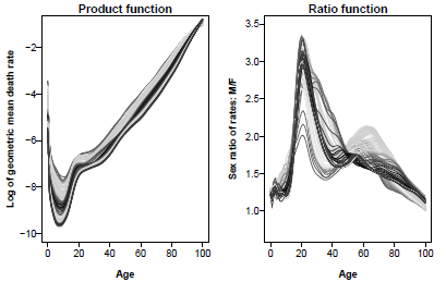
Observed(1950-2010) and forecast(2011-2030) product and ratio functions, U.S. mortality.
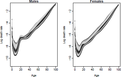
Observed(1950-2010) and forecast(2011-2030) male and female mortality rates using the product-ratio method with functional data models, United States.
8.6 Life Table Forecasting
The methods described in this chapter generate forecast mx rates, which can then be used to produce forecast life table functions using standard methods (e.g. Chiang 1984). Assuming that mx rates are available for ages 0,1,...,ω−1,ω+, the lifetable function in demography generates life table functions from a radix of l0=1 as follows for single years of age to ω−1:
qx=mx/(1+(1−ax)mx),(8.13)
dx=lxqx,(8.14)
lx+1=lx−dx,(8.15)
Lx=lx−dx(1−ax),(8.16)
Tx=Lx+Lx+1+⋅⋅⋅+Lω−1+Lω+, ex=Tx/lx,(8.18)
where ax=0.5 for x=1,...,ω−1, and a0 values (which allow for the fact that deaths in this age group occur earlier than midway through the year of age on average) are from Coale et al. (1983). For the final age group, qω+=1,Lω+=lx/mx, and Tω+=Lω+. For life tables commencing at an age other than zero, the same formulae apply, generated from a radix of 1 at the commencing age.
The demography package produces life tables using lifetable, and life expectancies using the function life.expectancy. For forecast life expectancies, flife.expectancy is used to produce the point forecast and the prediction interval. Additionally, e0 is a shorthand wrapper for flife.expectancy with age=0. The mx x rates on which the life table is based can be the rates applying in a future forecast year t, in which case a period or cross-sectional life table is generated, or can be rates that are forecast to apply to a certain cohort, in which case a cohort life table is generated. All functions use the cohort argument to give cohort rather than period life tables and life expectancies.
For example, to generate the cross-sectional life table for males in 1980, we use:
> lifetable(usa, series="male", year=1980, type="period")
Period lifetable for USA : male
Year: 1980
mx qx lx dx Lx Tx ex
0 0.0142 0.0140 1.0000 0.0140 0.9871 69.9883 69.9883
1 0.0011 0.0011 0.9860 0.0011 0.9854 69.0012 69.9835
2 0.0007 0.0007 0.9849 0.0007 0.9845 68.0157 69.0584
3 0.0006 0.0006 0.9842 0.0006 0.9839 67.0312 68.1089
4 0.0005 0.0005 0.9836 0.0004 0.9834 66.0473 67.1491
:
99 0.4066 0.3379 0.0051 0.0017 0.0043 0.0123 2.3891
100 0.4249 1.0000 0.0034 0.0034 0.0080 0.0080 2.3533
To generate the cohort life expectancy for males aged 65 by year in which aged 65 (using the coherent functional model obtained in Section 8.5), we use:
> usa.pr <- coherentfdm(smus1950.100, weight=TRUE, beta=0.05)
> usa.pr.f40 <- forecast(usa.pr,h=40)
> flife.expectancy(usa.pr.f40$male, age=65, type="cohort")
Point Forecast
1976 14.45048
1977 14.54158
1978 14.63950
1979 14.75728
1980 14.88563
2013 19.30161
2014 19.39335
2015 19.48484
To obtain prediction intervals for future life expectancies, we simulate the forecast log mortality rates as described in Hyndman & Booth (2008). Briefly, the simulated forecasts of log mortality rates are obtained by adding disturbances to the forecast basis function coefficients kt,j which are then multiplied by the fixed basis functions, bj(x) (assuming Equation 8.3). Then we calculate the life expectancy for each set of simulated log mortality rates. Prediction intervals are constructed from percentiles of the simulated life expectancies. This is all implemented in the demography package.
Using the coherent functional model obtained in Section 8.5, we can forecast period life expectancies (Figure 8.15) as follows:
> e0.fcast.m <- e0(usa.pr.f, PI=TRUE, series="male")
> e0.fcast.f <- e0(usa.pr.f, PI=TRUE, series="female")
> plot(e0.fcast.m, ylim=c(65,85), col="blue", fcol="blue", ylab="Years",
+ main="Product-Ratio method: coherent life expectancy forecasts")
> par(new=TRUE)
> plot(e0.fcast.f, ylim=c(65,85), col="red", fcol="red",main="")
> legend("topleft", lty=c(1,1),lwd=c(2,2), col=c("red", "blue"),
+ legend=c("female","male"))
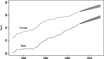
Observed(1950-2010) and forecast(2011-2030) male and female period life expectancy using the product-ratio method with functional data models, United States.
An alternative approach to life expectancy forecasting is direct modeling, rather than via mortality forecasts. This is the approach taken by Raftery et al. (2013) who use a Bayesian hierarchical model for life expectancy, and pool information across countries in order to improve estimates. Their model is implemented in the bayesLife package, available on CRAN.
8.7 Life Insurance Products
Connections between demographic functions, described in this chapter, and life contingencies (described in Chapter 7) can be made using the function probs2lifetable() in library lifecontingencies. The input used in this function is a vector of probabilities, either px or qx
To generate period qx rates that can be input into the lifecontingencies package, we simply use the lifetable function for either observed (past) or forecast rates:
> lifetable1980 <- lifetable(smus1950.100, series="male", year=1980, type="period")
> qx1980 <- lifetable1980$qx
> lifetable2025 <- lifetable(usa.pr.f$male, series="male", year=2025, type="period")
> qx2025 <- lifetable2025$qx
If we want to use cohort probabilities, we will in most cases need to use both observed mx,t and forecast ˆmx,t. Using the computations described above, and smoothed U.S. male rates at ages 0 to 100+ for 1950 to 2010, we obtain
> usa.pr <- coherentfdm(smus1950.100, weight=TRUE, beta=0.05)
> usa.pr.f150 <- forecast(usa.pr, h=150)
The matrix smus1950.100$rate$male contains past rates, mx,t, and usa.pr.f150$male $rate$male contains forecast rates, ˆmx,t. . We define the combined matrix, com.mx:
> com.mx <- cbind(smus1950.100$rate$male[1:nrow(usa.pr.f150$male$rate$male),], + usa.pr.f150$male$rate$male)
The cohort mortality rate for males born in 1950 is obtained using
> birthyear <- 1950
> mx <- com.mx[1:nrow(com.mx),(birthyear-1950+1):ncol(com.mx)]
> cohort.mx <- diag(mx)
> plot(log(cohort.mx), main="Cohort mortality rates, US males born in 1950",
+ ylab="Log death rate", xlab="Age")
Figure 8.16 shows the mortality rate surface as a function of x and t. The diagonal line is the cohort rate of mortality for males born in 1950.
> mat3d<-persp(seq(0,99,by=3),seq(1950,1950+209,by=5),
+ log(com.mx[seq(1,100,by=3),seq(1,210,by=5)]), theta=-30,
+ xlab="Age", ylab="Year", zlab="Log death rate", ticktype="detailed",
+ col=grey(.93), shade=TRUE)
> xyz3d <- tranS3d(0:100,birthyear+0:100, log(cohort.mx), mat3d)
> lines(xyz3d, col="red", lwd=2)
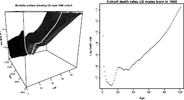
Observed (1950-2010) and forecast (2011-2150) rates, showing cohort rates for U.S. males born in 1950.
Based on vector cohort.mx, we compute qx using the equations given in Section 8.6. Note that Chapters 7 and 8 use slightly different assumptions for the construction of the life table, and therefore calculated life expectancy and other life table quantities will differ between the two for the same set of input qx rates.
8.8 Exercises
- 8.1 Download the Human Mortality Database (HMD) mortality data for Denmark and plot male mortality rates at single ages 0 to 95+ for the 20th century.
- 8.2 Using data from 1950 for Danish females aged 0-100+, smooth the data by the Currie-Durban-Eilers and Hyndman-Ullah methods. Plot the two smoothed curves and the observed data for 1950 and 2000.
- 8.3 Download HMD data for Canada. Using data for the total population, compare forecast life expectancy for the next 20 years from the Lee-Carter and Lee-Miller methods.
- 8.4 Apply the Booth-Maindonald-Smith method to total mortality data for Canada. What is the fitting period? How does this forecast compare with the Lee-Miller forecast in terms of life expectancy after 20 years?
- 8.5 Using female data for Japan (from HMD), apply the Hyndman-Ullah method and plot the first three components. Plot forecast mortality rates for the next 20 years. How does the forecast differ from a forecast of the same data using the Lee-Carter method without adjustment?
- 8.6 Using male data for Japan, apply the Hyndman-Ullah method to forecast 20 years ahead, and plot male and female observed and forecast life expectancies on the same graph.
- 8.7 Apply the product-ratio method of coherent forecasting to data by sex for Japan. Plot past and future product and ratio functions. Add coherent male and female forecast life expectancies to the previous life expectancy graph.
- 8.8 Plot the sex difference over time in observed life expectancy, in independently forecast life expectancy and in coherently forecast life expectancy.
1For clarity, models have been written in a standardised format which may in some cases differ from the form used by the authors originally. ax and bx terms are used for age-related effects, kt terms for period-related effects, and γt-x terms for cohort-related effects. Models originally expressed in terms of the force of mortality are expressed in terms of the central death rate; these are equivalent under the assumption of a constant force of mortality over each year of age.