Chapter 12

Yield Curves and Interest Rates Models

Sergio S. Guirreri

Accenture S.p.A.
Milan, Italy

12.1 A Brief Overview of the Yield Curve and Scenario Simulation

In recent years, the simulation of scenarios of macroeconomic variables has became a crucial issue. Institutional operators, such as national banks, insurance companies, and investment banks must evaluate different scenarios of financial and macroeconomic variables before adopting a monetary policy or promoting a new pension plan. Economic variables such as interest rates and monetary aggregates are often studied by economists to forecast the path of the economy or to predict an ongoing recession. The relationship among interest rates at different maturities contains relevant information about future economic activities. A research of the Federal Reserve Bank (Estrella & Mishkin (1996)) emphasizes the role of the yield curve as a predictor of an ongoing recession. There is a strong relationship among the yield curve, monetary policy, and investor expectations. The monetary policy and the changes in investor expectations affect the slope of the term structure of interest rates; therefore it has been shown that the role of the yield curve is as an indicator of an ongoing recession, or to forecast the future inflation (Estrella & Ttubin (2006)). The interest rates are also used for other purposes such as pricing derivatives, evaluating investment projects, or computing risk measures; thus, a good representation of the evolution of the yield curve in the long horizon is a key risk factor for decision makers.

Scenarios of the yield curve represent different states of the world economy; therefore a simulation model of the yield curve is a useful tool, both for a decision makers and for a forecaster. In fact, the more trustworthy are the scenarios simulated and the more accurate will be the risk assessment of a future choice for a decision maker, while for a forecaster the more accurate will be the forecasting model.

In continuous-time classical actuarial pricing, the value (at time t) of a future payoff (as time τ > t) denoted $F_{\tau }\text{ is }{V}_t\left(F_{\tau }\right)=e^{-r\left(\tau -t\right)}{F}_{\tau }$ where r denotes the discount factor, or interest rate. In Chapter 7, a discrete interest rate was considered, and was denoted i. In that context, if t and Y are discrete, $V_t\left(F_{\tau }\right)={(1+i)}^{-(\tau -t)}{F}_T$ But in both cases, r and i were considered as constant, which might not be realistic. Thus, more generally, one can assume that $V_t\left(F_{\tau }\right)=B(t,{\rm T})F_{\tau }$ where B(t,τ) is the value of a risk-free asset, at time t, that will pay 1 at time τ (with τ > t). This product is usually called a zero-coupon bond. If such products were exchanged on markets, for all possible maturities τ, and all times t, then prices of those bounds could be used as discount factors. Unfortunately, only some of them can be observed, and therefore it is necessary to extrapolate B(t, τ)'s based on some observed values.

But more than zero-coupon prices, it may be interesting to model instantaneous (stochas­tic) rates $r_s$ , such that

$V_t\left(F_{\tau }\right)={\text{?}}_{\text{ℚ}}\left(\exp \left(\int {}_t^{\tau }{r}_{s}ds\right)F_{\tau }\right)$ ,

where Q denotes the risk-neutral measure (assumed here to be unique; see Privault (2008) for more details).

At time t, the dynamic of forward rates is given either by the yield to maturity curve, defined as

$\tau \mapsto y(t,\tau )=\frac{1}{\tau -t}\int \begin{array}{c}\tau \\ t\end{array}{r}_{s}ds$

or instantaneous forward curve, defined as

$\tau \mapsto y_f(t,\tau )=-\frac{\partial }{\partial \tau }\log B(t,\tau )=-\frac{\partial }{\partial \tau }\log \left(\exp \left(\int \begin{array}{c}\tau \\ t\end{array}{r}_{s}ds\right)\right)$ .

For convenience, in this chapter, we will consider the case where t = 0, and denote yf (t) and y(t,τ), respectively, the instantaneous forward rate, and the yield to maturity.

The financial and economic literature have proposed two different frameworks to fit the evolution of the yield curve. The first one is based on term-structure models designed for pricing purposes (Vasicek (1977), Cox et al. (1985), Duffie & Kan (1996)). In Vasicek (1977), short rate is supposed to satisfy

$d{r}_t=a\left(b-r_t\right)dt+\sigma d{W}_t$ ,

while in Cox et al. (1985),

$d{r}_t=a\left(b-r_t\right)dt+\sqrt{r_t}\sigma d{W}_t$ .

The second one is based models that attempt to provide a statistical description of the evolution of rates in the objective measure (Nelson & Siegel (1987), Svensson (1994)). Recently, it has been shown (Diebold & Li (2006)) that a dynamic approach based on the factor of Nelson-Siegel's model can reproduce key features of U.S. interest rate curves with good forecasting performances.

Some key factors of the yield curve are that the linear correlation between the short and long term rates, and correlations at different lags, are very high; the marginal distributions of the yield curve differ from the Normal distribution; and the time series of each interest rate are not stationary. Some statistical methodologies that have been recently applied to estimate the previous features of the term structure of interest rates are the vector auto­regressive model (VAR) and the copula approach.

In particular the VAR model is able to capture most of the key factors of the yield curve such as the cross and lagged correlation, but it is limited to simulating the interest rates because the marginal distributions are assumed Gaussian (Ang & Piazzesi (2003)). The marginal distributions of interest rates are significantly different from the Gaussian distribution, especially when, by the first differences, the interest rates are transformed into stationary time series. For this reason, the Gaussian vector auto-regressive model is not able to capture the entire feature of the term structure interest rates.

The copula method (Cherubini et al. (2004)) allows us to model the dependence structure independently of the marginal distributions. One may construct a multivariate distribution with different marginals with the copula function that describes the dependence structure. The main limit of the model based on this approach is that they focused on estimating copula, when data are dependent, and did not supply the VAR dynamics.

Recently, a new methodology has been proposed to generate the scenario of the term structure of interest rates (Consiglio & Guirreri (2011)) using the VARTA (Vector Au­toregressive To Anything) approach of Biller & Nelson (2003). In this framework, the two authors are able to simulate a scenario of the yield curve in the long horizon replicating: the correlation among interest rates, the autocorrelation at different lags of each rate time series, and the marginals distribution, using the Johnson' distributions (Johnson (1949)). The non-stationarity of the interest rates time series is one limit of the IRTA (Interest Rates To Anything) methodology, whereas the second one is the number of interest rates that the IRTA is able to simulate. The latter issue can be solved by simulating the coefficients of Nelson-Siegel's model, using the VARTA approach, and then build the term structure of the interest rates using the number of pillars as input (Guirreri (2010)).

Rebonato et al. (2005) emphasize the role of the scenarios simulation of the yield curve in the real world. The yield curve is a key factor in numerous applications; some examples are the following:

• Evaluation of potential future exposure (PFE) for counter party credit risk assessment: In order to evaluate the PFE, the relevant yield curve must be simulated, typically using a Monte Carlo procedure, and the conditional exposure in the various states of the world computed.
• Assessment of the hedging performance of interest rate option models: In this context, one wants to judge the quality of a model from its assumptions. One method is to shock the real-world yield curve by a few eigenvalues obtained from the orthogonalization of the covariance matrix. The hedging strategy suggested by a simple diffusive pricing model with deterministic volatilities will produce a good replication of the payoff of a plain-vanilla option. This is more likely to be due, however, to the very simplified nature of the yield curve evolution rather than to any intrinsic virtues of the modeling approach.
• Assessment of different investment strategies in interest rate-sensitive investment portfolios (Asset/Liability management): Investment portfolios are usually evaluated with reference to the net interest income (NII) that they generate. It is not a complex issue to generate a favorable NII over a short period of time, but it is essential to compare the NII performance of competing interest rate-based portfolios, evaluating over a suitably long time horizon.
• Economic capital calculations: These techniques estimate the marginal contribution of a new investment or a business activity to a total loss profile. In these applications, the evolution of the yield curve plays an important role because the loss profile is affected by the interest rates not only directly, but also indirectly via the depositors' behavior or mortgage prepayment patterns.

There are three main reasons why scenario analysis is often preferred over alternative approaches (Steehouwer (2005)). The first reason is the flexibility it offers to model the often complex interactions and relations within and between the components of an ALM problem.

The second reason for the popularity of scenario analysis is that it offers great possibil­ities for learning about the problem under consideration in addition to just obtaining some “optimal” solution.

The third reason is that the strong visual aspects of scenario analysis cause the models and the solutions obtained to be more easily accepted by decision makers. In conclusion, the scenarios play an important role in strategic policy-making processes of institutions such as pension funds, insurance companies, and banks.

Macroeconomic scenarios are fundamental inputs for Asset and Liability Management (ALM) models. The output of ALM models strongly depends on the input scenarios. For this reason, it is of paramount importance to have a scenario generator as reliable as possible. Reliability, in this respect, means that the distribution of the set of scenarios resembles as much as possible the empirical one.

The concepts of scenario analysis, also called Monte Carlo simulation or stochastic simulation, are often applied to study financial tools and modeling the economic risk and return factors. An economic scenario is a possible future evolution of all relevant (uncertain) macroeconomic (and other) variables. Usually, a large number of scenarios of economic variables is generated, for example, several hundreds with a horizon of 15 years. Together with the strategic policy under consideration, these are fed into a model that states all relations between policy instruments, scenario variables, and relevant output measures with respect to the objectives of the stakeholders1. With the system of the above relations at hand, the model simulates what would happen to the objectives of the stakeholders if the policy under consideration were applied during the simulation period. For example, the output of the model could be the future evolution of the solvency ratio of an insurance company for each of the economic scenarios.

It is important to note that the scenarios should be neutral with respect to the ob­jectives and constraints of the various stakeholders. The scenarios represent one and the same independent, macroeconomic world in which the economic entity under investigation and its stakeholders need to operate and which they cannot change by themselves. Based on the scenarios, different risk and return measures can be calculated. Examples of such measures are the probability of the solvency ratio falling below the legally required 100% (a risk measure) or the expected return on equity during the next 15 years (a return measure). In the next step, decision makers have to evaluate these risk and return numbers of the policy under consideration and decide whether, for example, the expected return on equity is above or below the expectations.

The following sections will focus on the Nelson-Siegel's model and Svensson's model using the R package YieldCurve; see Guirreri (2012)

12.2 Yield Curves

12.2.1 Description of the Datasets

Interest rates of the central bank of the United States, the Federal Reserve, can be down­loaded from the Fed website 2 selecting the variables in scope. We will use, for different dates t and different maturities $\tau$ , interest rates $y\left(t,\tau \right)$ . Usually, maturities are given (1 year, 2 years, 10 years, etc.), and thus, for all maturities, we do have a time series $t\mapsto y\left(t,\tau \right)$ . In­terest rates are a collection of time series $\left(y\left(t,\tau \right)\right)$ . One can either use functional time series from the ftsa library (as in Chapter 9), or extensible time series from the xts library. The package YieldCurve involves the following datasets:

1. FedYieldCurve: an xts object that contains the interest rates of the Federal Reserve, from January 1982 to December 2012. The interest rates are Market yield on U.S. Treasury securities constant maturity (CMT)3 at different maturities (3 months, 6 months, 1 year, . . . , 10 years), quoted on investment basis and have been gathered with monthly frequency.
2. ECBYieldCurve: an xts object that consists of a collection of interest rates of the European Central Bank 4 at different maturities.

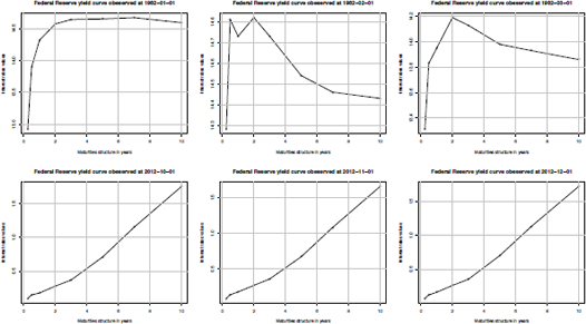
We visualized the Fed yield curve at the several selected dates. Indeed, the first 3 and the last 3 months were selected from the dateset FedYieldCurve.

>  require(xts)

>  require(YieldCurve)

>  data(FedYieldCurve)

>  first(FedYieldCurve,'3 month')

   R_3M  R_6M R_1Y R_2Y R_3Y R_5Y  R_7Y R_10Y

1982-01-01 12.92  13.90 14.32  14.57 14.64 14.65 14.67 14.59

1982-02-01 14.28  14.81 14.73  14.82 14.73 14.54 14.46 14.43

1982-03-01 13.31  13.83 13.95  14.19 14.13 13.98 13.93 13.86

>   last(FedYieldCurve,'3 month')

   R_3M  R_6M R_1Y R_2Y  R_3Y  R_5Y  R_7Y R_10Y

2012-10-01 0.10  0.15  0.18 0.28 0.37   0.71  1.15  1.75

2012-11-01 0.09  0.14  0.18 0.27 0.36   0.67  1.08  1.65

2012-12-01 0.07  0.12  0.16 0.26 0.35   0.70  1.13  1.72

>  mat.Fed<-c(3/12, 0.5, 1,2,3,5,7,10)

>  par(mfrow=c(2,3))

>  for(i in c(1,2,3,370,371,372)){

+ plot(mat.Fed, FedYieldCurve[i,], type="o",

xlab="Maturities structure in years", ylab="Interest rates values")

+ title(main=paste("Federal Reserve yield curve observed at", time(FedYieldCurve[i], sep=" ")))

+ grid()

}

The interest rate surface can also be visualized in Figure 12.2.

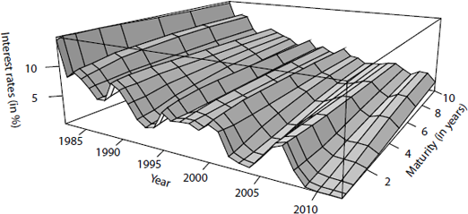
> persp(1982:2012,maturity,FedYieldCurve[seq(2,nrow(FedYieldCurve),by=12),],

+ theta=30,xlab="Year",ylab="Maturity (in years)",

+ zlab="Interest rates (in %)",ticktype = "detailed",shade=.2,expand=.3)

12.2.2 Principal Component Analysis

As mentioned previously in Vasicek (1977), the short rate is modeled, assuming that $d{r}_t=a\left(b-r_t\right)dt+\sigma d{W}_t$ , and the the rest of the curve is derived from it. This can be seen as a one-factor model. But it is clearly not enough to obtain stylized facts discussed in the previous section. Litterman & Scheikman (1991) looked at the treasury yield curve, and obtained that only a few factors were necessary because only a three eigenvalues were significant. Those three factors could actually be used to model the level of the yield curve, the slope of the curve, and the curvature of the curve.

To perform a principal component analysis, let $\mathit{Y}=\left[{\mathit{Y}}_1,\mathrm{...},{\mathit{Y}}_m\right]$ be the collection of all time series, in matrix form. Vector ${\mathit{Y}}_j$ is the time series associated to jth maturity. Classically, we should normalize the data by subtracting the mean from each of the data dimensions. The goal is to find the linear combination of the ${\mathit{Y}}_j$ 's with maximum variance. Thus, we have to solve

$\underset{||\mathit{u}||=1}{\max }\left\{{\mathit{u}}^{\prime }{\mathit{X}}^{\prime }\mathit{X}\mathit{u}\right\}.$

Because ${\mathit{X}}^{\prime }\mathit{X}$ is a positive definite matrix, it admits a decomposition $\mathit{P}\mathit{\Delta }{\mathit{P}}^{\mathit{\prime }}$ , where P is an orthogonal matrix, and $\mathit{\Delta }$ is a diagonal matrix, containing all eigenvalues. Assume that eigenvalues are ordered in decreasing order, $\mathit{\Delta }=\text{diag}\left({\lambda }_1,\cdots ,{\lambda }_m\right),then {\lambda }_1\ge \cdots \ge {\lambda }_n>0$ (because ${\mathit{X}}^{\mathit{\prime }}\mathit{X}$ is positive definite). Let F = XP. Columns of F are called factors. By construction, note that those factors are orthogonals. And the ${\mathit{X}}_t$ 's are linear combinations of the factors because $\mathit{X}=\mathit{F}{\mathit{P}}^{\mathit{\prime }}$ :

${\mathit{X}}_t=\sum _{j=1}^m{\mathit{P}}_{j,t}{\mathit{F}}_j.$

To perform such a decomposition, use the princomp function:

>   M <- as.matrix(FedYieldCurve)

>   pca.rates <- princomp(M, scale=TRUE)

As mentioned previously, three factors are clearly sufficient, as those first three explain 99.9% of the total variance,

>   summary(pca.rates)

>   summary(pca.rates)

Importance of components:

        Comp.1  Comp.2  Comp.3   Comp.4

Standard deviation   8.5598756 1.16055974 0.2557040238 0.1246520910

Proportion of Variance   0.9808032  0.01802943 0.0008752298 0.0002079918

Cumulative Proportion  0.9808032 0.99883266 0.9997078851 0.9999158769

        Comp.5    Comp.6   Comp.7  Comp.8

Standard deviation   5.544781e-02  3.941926e-02  0.0341450611  2.214145e-02

Proportion of Variance   4.115435e-05 2.080003e-05  0.0000156064  6.562348e-06

Cumulative Proportion  9.999570e-01  9.999778e-01  0.9999934377 1.000000e+00

The three factors can be visualized in Figure 12.3.

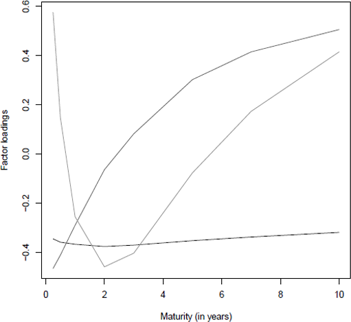
>   factor.loadings <- pca.rates$loadings[,1:3]

>   matplot(maturity,factor.loadings,type="l", lwd=c(2,1,1),

+ lty=c(1,1,2),xlab = "Maturity (in years)", ylab = "Factor loadings")

The first one is (almost) flat and corresponds to the level of the yield curve. The second one is a monotone function, which will explain the slope of the curve. And the third one is a convex function that will explain the curvature of the curve.

The evolution of weights ${\mathit{P}}_{j,t}$ for j = 1, 2, 3 can be visualized in Figure 12.4.

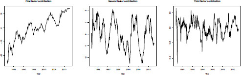
>   vtime=seq(1981+11/12,length=nrow(M),by=1/12)

>   for(j in 1:3) plot(vtime,pca.rates$scores[,j],type="l",xlab="Year")

12.3 Nelson—Siegel Model

The core of this section is the Nelson-Siegel model and the dynamic approach used by Diebold & Li (2006) to model and forecast the yield curve. The Nelson-Siegel model is widely used among central banks and financial analysts, and its popularity is due to its flexible and parsimonious form. In Diebold & Li (2006), it is observed that the Nelson- Siegel model fits both the cross section and time series of yields remarkably well, in many countries and periods. They described the yield curve evolution using the Nelson-Siegel model, giving an interpretation to the three factors as level, slope, and curvature of the term structure interest rates. To model the dynamics of the whole yield curve, Diebold and Li estimate an auto-regressive model for each of the three coefficients.

The aim of Nelson & Siegel (1987) was to define a parsimonious model to be flexible enough to describe the various shapes and features of the yield curve. The most frequent shapes of the yield curve are the humped and S forms. Nelson and Siegel focused on a class of functions that could be able to generate the typical form of the yield curve. This class of functions is related to the Laguerre functions, which consist of a polynomial term and an exponential decay term. The instantaneous forward rate, yf, at maturity $\tau$ is described by the following relation:

$yf\left(\tau \right)={\beta }_0+{\beta }_1\exp \left(-\frac{\tau }{\dot{\lambda }}\right)+{\beta }_2\left[\frac{\tau }{\dot{\lambda }}\exp \left(-\frac{\tau }{\dot{\lambda }}\right)\right](12.1)$

where $\dot{\lambda }$ is a time constant related to the maturity $\tau$ and $\left({\beta }_0,{\beta }_1,{\beta }_2\right)$ are unknown param­eters. Equation (12.1) can be viewed as a constant plus a Laguerre function (see furthers details in Heiberger & Neuwirth (1953)). The yield to maturity can be obtained from the instantaneous forward rate:

$y\left(\tau \right)=\frac{1}{\tau }\int {}_0^{\tau }yf\left(x\right)dx(12.2)$

Substituting Equation (12.1) in (12.2) and solving the integral, we obtain the Nelson-Siegel yield curve:

$y\left(\tau \right)={\beta }_0+{\beta }_1\left(\frac{1-\exp \left(-\frac{\tau }{\dot{\lambda }}\right)}{\frac{\tau }{\dot{\lambda }}}\right)+{\beta }_2\left(\frac{1-\exp \frac{\tau }{\dot{\lambda }}}{\frac{\tau }{\dot{\lambda }}}-\exp \left(-\frac{\tau }{\dot{\lambda }}\right)\right),(12.3)$

where ${\beta }_0$ represents the long-term component that does not decay to zero in the limit.

The coefficient ${\beta }_1$ has the loading factor

$\frac{1-\exp \left(-\frac{\tau }{\dot{\lambda }}\right)}{\frac{\tau }{\dot{\lambda }}}$

that approaches 1 as $\tau \to 0$ and decays quickly to 0 as $\tau \to 0+\infty ;$ hence ${\beta }_1$ identifies the short-term component.

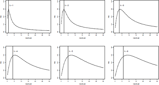
The factor loading of ${\beta }_2$ models a hump shape, starting at zero and reaching its maximum and then decreasing to zero; thus the coefficient ${\beta }_2$ can be viewed as the medium-term factor. It is interesting to note that the instantaneous yield is governed by the long and short term, $y\left(0\right)={\beta }_0+{\beta }_1$ .

The parameter $\dot{\lambda }$ controls the decay of the regressors and determines at which maturity the medium-term factor reaches its maximum, namely the position of the hump. In partic­ular, large values of $\dot{\lambda }$ produce slow decay in the regressors and better fitting on the longer maturity, while small values of $\dot{\lambda }$ produce a quick decay in the regressors and a better fit on the short maturity.

The following R code will help us to understand the role of each component of Equation (12.3):

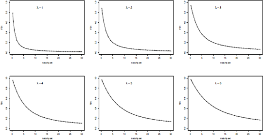
>   factorBeta1 <- function(lambda, Tau)

+ {

+   (1-exp(-Tau/lambda)) / (Tau/lambda)

+}

>   maturity.set<-c(3/12,6/12,seq(1:30))

>   lambda.set <- c(0.5,i,2,3,4,5)

>   par(mfrow=c(2,3))

>   for(i in 1:length(lambda.set)){

+ FB1 <- factorBeta1(lambda.set[i],maturity.set)

+ plot(maturity.set, FB1, type="o", ylim=c(0,i))

+ text(12,0.9, substitute(list(lambda) == group("",list(x),MM),list(x=i)),cex=1.5)

+}

>  factorBeta2 <- function(lambda, Tau)

+ {

+ (1-exp(-Tau/lambda)) / (Tau/lambda) - exp(-Tau/lambda)

+}

>   par(mfrow=c(2,3))

>  for(i in 1:length(lambda.set)){

+ FB2 <- factorBeta2(lambda.set[i],maturity.set)

+ plot(maturity.set, FB2, type="o", ylim=c(0,0.4))

+ text(i+2,0.35, substitute(list(lambda) == group("",list(x),""),list(x=i)),

  cex=1.5)

+ abline(v=i, lty=2)

+}

Therefore, the loading factors of ${\beta }_1$ and ${\beta }_2$ depend on $\tau$ , that is, a set of maturities for which we want to represent the rate curve, and λ , that is, an unknown key factor for the Nelson-Siegel model. More generally, to fit, Equation (12.3) should use nonlinear methods to estimate the set of unknown parameters $\left({\beta }_0,{\beta }_1,{\beta }_2,\dot{\lambda }\right)$ , when facing some problem related to this method, such as time computing, performance, constrains verification.

To avoid the implementation of some nonlinear optimization algorithms, the R package YieldCurve has been used as one of the ideas behind the paper of Diebol-Li. The two main ideas of Diebold & Li (2006) were

1. Estimating the Nelson-Siegel model as a linear model,fixing a $\dot{\lambda }$ value for each period;
2. Forecasting the term structure of interest rates based on the parameters of the Nelson-Siegel model, instead of each single interest rate used in the structure of the rate curve.

The first point was developed in the function NelsonSiegel() of the R package YieldCurve fixing a grid of $\dot{\lambda }$ and for each value an estimate of the Nelson{Siegel model, by ordinary least square (OLS), has been obtained. The best estimate of $\widehat{\lambda }$ is the value that maximizes the medium-term factor loading:

${\max }_{{\dot{\lambda }}_j}\left[\frac{1-\exp \left(-\frac{{\tau }_j}{{\dot{\lambda }}_j}\right)}{\frac{{\tau }_j}{{\dot{\lambda }}_j}}-\exp \left(-\frac{{\tau }_j}{{\dot{\lambda }}_j}\right)\right],j=1,\mathrm{...},n (12.4)$

In correspondence with each ${\widehat{\lambda }}_j$ I is estimated by OLS parameters $\left({\widehat{\beta }}_{0,j},{\widehat{\beta }}_{1,j},{\widehat{\beta }}_{2,j}\right)$. The best fitting of the Equation (12.3) is obtained for parameters $\left({\widehat{\beta }}_0,{\widehat{\beta }}_1,{\widehat{\beta }}_2,\widehat{\lambda }\right)$ that minimize the sum of the square of residuals:

${\min }_{{\widehat{\beta }}_{0,j},j,{\widehat{\beta }}_{1,j},{\widehat{\beta }}_{2,j},{\widehat{\lambda }}_j}{\sum _j\left[yobs-{\widehat{y}}_j\left(\tau \right)\right]}^2,j=1,\mathrm{...},n,(12.5)$

where yobs is the yield curve observed and ${\widehat{y}}_j\left(\tau \right)$ corresponds to the yield curve fitted by the Nelson-Siegel model with the parameters $\left({\widehat{\beta }}_{0,j},{\widehat{\beta }}_{1,j},{\widehat{\beta }}_{2,j},{\widehat{\lambda }}_j\right)$. The above estimation method avoids a non-trivial problem due to the presence of multiple local optima in the cross section of coupon bond prices, as the function to optimize is not guaranteed to be convex.

12.3.1 Estimating the Nelson-Siegel Model with R

The estimation of the yield curve shown in the graph (12.1) can be done using the Nelson- Siegel model (12.3) implemented in the function Nelson.Siegel(), where the input argu­ments are

• rate: It can be a vector or a matrix with interest rates observed at several periods, one row for each day. The default class of the rate object is xts.
• maturity: It is a vector that represents the structure of the interest rate and it must have the same length as the number of columns of the rate object.

Recall that at time t, Equation (12.3) is

$y\left(t,\tau \right)={\beta }_0\left(t\right)+{\beta }_1\left(t\right)\left(\frac{1-\exp \left(-\frac{\tau }{\dot{\lambda }\left(t\right)}\right)}{\frac{\tau }{\dot{\lambda }\left(t\right)}}\right)+{\beta }_2\left(t\right)\left(\frac{1-\exp \left(-\frac{\tau }{\dot{\lambda }\left(t\right)}\right)}{\frac{\tau }{\dot{\lambda }\left(t\right)}}-\exp \left(-\frac{\tau }{\dot{\lambda }\left(t\right)}\right)\right)\cdot \left(12.6\right)$

Thus, at each time t, four coefficients are estimated:

>   Fed.Ratel <- Nelson.Siegel(first(FedYieldCurve, '3 month'), mat.Fed)

>   Fed.Rate1

	  beta_0  beta_1  beta_2  lambda

1982-01-01 14.34594  -1.76249751  3.650061 0.9999507

1982-02-01 14.14681 0.05426534  2.219142 0.9999507

1982-03-01 13.61065  -0.54316951  2.708078 0.9999507

>   Fed.Rate2 <- Nelson.Siegel(last(FedYieldCurve, '3 month'), mat.Fed)

>   Fed.Rate2

	   beta_0 beta_1 beta_2 lambda

2012-10-01 6.752246  -6.62480  -6.609233 0.183919

2012-11-01 6.292996  -6.17330  -6.111852 0.183919

2012-12-01 6.590762  -6.49626  -6.364102 0.183919

The output of the function is the estimation of the Nelson-Siegel coefficients and the λ parameter for each period. Comparing the coefficients of the two outputs, Fed.Rate1 and Fed.Rate2, can be noted as the long-run component ${\widehat{\beta }}_0$ , has d significantly change; and, in the same way, the slope and the curvature of the yield curve.

Proceeding with the estimation of the yield curve for each period in the dataset FedYieldCurve, one can observe the behavior of the multivariate time series of the Nelson- Siegel coefficient to obtain some information on the trend of the term structure of interest rates.

>   system.time(Nelson.Siegel(FedYieldCurve, mat.Fed))

 user system elapsed
 18.93 0.08  19.30

>   Fed.Rates <- Nelson.Siegel(FedYieldCurve, mat.Fed)

>   first(Fed.Rates,'year')

	   beta_0   beta_1  beta_2 lambda

1982-01-01 14.34594 -1.76249751 3.65006071 0.9999507

1982-02-01 14.14681 0.05426534 2.21914158 0.9999507

1982-03-01 13.61065 -0.54316951 2.70807842 0.9999507

1982-04-01 13.61517 -0.51818755 2.75748648 0.9999507

1982-05-01 13.52630 -1.16619236 2.39279341 0.9999340

1982-06-01 14.13378 -1.43747932 3.23769741 0.9999507

1982-07-01 13.84696 -2.49133196 3.69440615 0.9999507

1982-08-01 13.02162 -4.77732118 4.90917816 0.9999507

1982-09-01 12.10749 -4.77732737 6.11249115 0.9999507

1982-10-01 11.02616 -3.75388964 2.73096552 0.9999340

1982-11-01 10.80609 -2.77592647 0.51759030 0.9999507

1982-12-01 10.84695 -2.96572285 0.05023213 0.9999507

>  last(Fed.Rates,'year')

	   beta_0   beta_1  beta_2 lambda

2012-01-01 5.067016 -5.002900  -5.291108 0.2869276

2012-02-01 5.415061 -5.293744  -5.645563 0.2656801

2012-03-01 5.266186 -5.166166  -5.092655 0.2869276

2012-04-01 5.520023 -5.401772  -5.608334 0.2656801

2012-05-01 6.755632 -6.641670  -6.408147 0.1839190

2012-06-01 5.829454 -5.717205  -5.360561 0.1839190

2012-07-01 5.942878 -5.805087  -5.918784 0.1839190

2012-08-01 6.007142 -5.890642  -5.770203 0.1938867

2012-09-01 6.877328 -6.739946  -6.945611 0.1839190

2012-10-01 6.752246 -6.624800  -6.609233 0.1839190

2012-11-01 6.292996 -6.173300  -6.111852 0.1839190

2012-12-01 6.590762 -6.496260  -6.364102 0.1839190

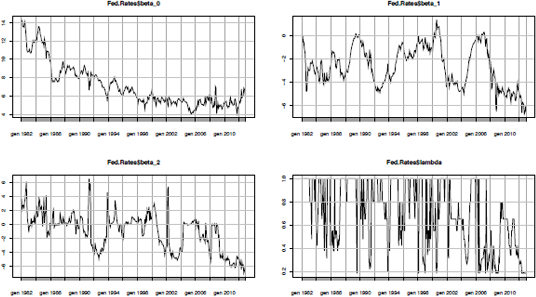
>  par(mfrow=c(2,2))

>  plot(Fed.Rates$beta_0, main='Beta_0 coefficient', ylab='Values')

>  plot(Fed.Rates$beta_1, main='Beta_1 coefficient', ylab='Values')

>  plot(Fed.Rates$beta_2, main='Beta_2 coefficient', ylab='Values')

>  plot(Fed.Rates$lambda, main='Lambda coefficient', ylab='Values')

From the trend of the ${\beta }_0$ it is evident that the long-term interest rate decreases during the last years, the time series of the slope, ${\beta }_1$ , increases over the crisis period, while the hump of the term structure is located in the long period5 and tends to be an inverted hump.

To obtain the interest rates from the Nelson-Siegel estimates, they have developed the function NSrates(), where the input variables are

1. Coeff: A vector or matrix of the Nelson-Siegel function, such as returned from the Nelson.Siegel(), indeed the Fed.Rates object.
2. maturity: A vector that represents the structure of the yield curve, indeed the mat.Fed object.

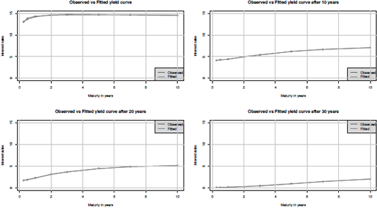
For example, if we want to obtain the estimated interest rates, we can run the following code:

>   Fed.yield.curve <- NSrates(Fed.Rates, mat.Fed)

>   par(mfrow=c(2,2))

>   plot(mat.Fed, as.numeric(FedYieldCurve[1,]), type="o", col=2,

+ ylab="Interest rates", xlab="Maturity in years", ylim=c(0,15))

>   lines(mat.Fed, as.numeric(Fed.yield.curve[1,]), type="o", col=3)

>   title(main="Observed vs Fitted yield curve")

>   legend('bottomright', legend=c("Observed","Fitted"),col=c(2,3), lty=1, bg='gray90')

>   grid()

>   plot(mat.Fed, as.numeric(FedYieldCurve[120,]), type="o", col=2,

+ ylab="Interest rates", xlab="Maturity in years", ylim=c(0,i5))

>   lines(mat.Fed, as.numeric(Fed.yield.curve[120,]), type="o", col=3)

>   title(main="Observed vs Fitted yield curve after 10 years")

>   legend('bottomright', legend=c("Observed","Fitted"),col=c(2,3), lty=1, bg='gray90')

>   grid()

>   plot(mat.Fed, as.numeric(FedYieldCurve[240,]), type="o", col=2,

+ ylab="Interest rates", xlab="Maturity in years", ylim=c(0,15))

>   lines(mat.Fed, as.numeric(Fed.yield.curve[240,]), type="o", col=3)

>   title(main="Observed vs Fitted yield curve after 20 years")

>   legend('topright', legend=c("Observed","Fitted"),col=c(2,3), lty=1, bg='gray90')

>   grid()

>   plot(mat.Fed, as.numeric(FedYieldCurve[360,]), type="o", col=2,

+ ylab="Interest rates", xlab="Maturity in years", ylim=c(0,15))

>   lines(mat.Fed, as.numeric(Fed.yield.curve[360,]), type="o", col=3)

>   title(main="Observed vs Fitted yield curve after 30 years")

>   legend('topright', legend=c("Observed","Fitted"),col=c(2,3),

+ lty=1, bg='gray90')

>   grid()

The graphic in Figure 12.8 shows the evolution of the yield curve since 1982 in steps of 10 years. [It is evident as the curve is shifted down, ${\beta }_0$ coefficient, whereas the curvature, ${\beta }_2$ coefficient, is changed from a “positive” to “negative” hump.] To better understand therole of each coefficient of the Nelson-Siegel model we can run the following code for the curvature using the estimated value of the last period and keeping fixed all other coefficients:

>   last(Fed.Rates,'month')

   beta_0 beta_1  beta_2 lambda

2012-12-01 6.590762 -6.49626 -6.364102  0.183919

>   b0<-rep(6.590762,21)

>   b1<-rep(-6.496260,21)

>   b2<-seq(-10, 10,by=1) # create a sequence of fictive beta_2 coeff

>   lambda<-rep(0.1839190,21)

>   B<-ts(cbind(b0,b1,b2,lambda), start=c(2000,1,1),

+ frequency=12)#create a time series object

>   B<-as.xts(B,REclass="FALSE)# trasform the time series object in xts

>   A<- NSrates(B ,mat.Fed)#create the fictive yield curves

#   create an interactive plot shows the movement of the yield curve

#   at different values of beta_2

>   for(i in 1:nrow(A))

+ {

+ plot(mat.Fed, A[i,],type="l", ylim=c(-1,6))

+ title(main=paste("beta_2",B[i,3], sep="="))

+ par(ask=TRUE)

+}

12.4 Svensson Model

12.4.1 Estimating the Svensson Model with R

The Nelson-Siegel model has optimal performance and returns good results if the maturities are not longer than 15 years. When the term structure is more complex, fitting by the Nelson-Siegel model is unsatisfactory. This is due to the convexity effect that tends to pull down the yields on longer-term securities, giving the yield curve a concave shape at longer maturities. Svensson proposed an extension of the Nelson-Siegel approach by increasing its flexibility and improving the fitting on a richer term structure. Svensson methodology assumes that the spot rates are governed by six parameters according to the following functional form:

$y\left(\tau \right)={\beta }_0+{\beta }_1\left(\frac{1-\exp \left(-\frac{\tau }{{\lambda }_1}\right)}{\frac{\tau }{{\lambda }_1}}\right)+{\beta }_2\left(\frac{1-\exp \left(-\frac{\tau }{{\lambda }_1}\right)}{\frac{\tau }{{\lambda }_1}}-\exp \left(-\frac{\tau }{{\lambda }_1}\right)\right)+{\beta }_3\left(\frac{1-\exp \left(-\frac{\tau }{{\lambda }_2}\right)}{\frac{\tau }{{\lambda }_2}}-\exp \left(-\frac{\tau }{{\lambda }_2}\right)\right)(12.7)$

Equation (12.7) is equal to Equation (12.3) when ${\beta }_3$ is set to zero. The factor loading of the coefficient ${\beta }_3$ captures a second “hump” of the yield curve at longer maturities, and ${\lambda }_2$ indicates the position of the second hump. A survey of the Bank for International Settlements (2005) showed that many central banks use the Nelson-Siegel-Svensson model to describe the evolution of the yield curve.

The estimation methodology implemented in the R package YieldCurve is similar to that used for the Nelson-Siegel model:

1. Two vectors of maturities, in the medium- and long-term ranges, have been selected: ${\omega }_1={\left(1,\mathrm{...},n_1\right)}^{\text{'}}\text{and }{\omega }_2={\left(1,\mathrm{...},n_2\right)}^{\text{'}}$
2. A grid of estimations of ${\lambda }_1\text{ and }{\lambda }_{\text{2}}$ is obtained, respectively, by maximizing the ${\beta }_1\text{ and }{\beta }_{\text{3}}$ factor loadings:
   

   ${\widehat{\lambda }}_{1j}=\underset{{\lambda }_1}{\max }\left[\frac{1-\exp \left(-\frac{{\omega }_{1j}}{{\lambda }_1}\right)}{\frac{{\omega }_{1j}}{{\lambda }_1}}-\exp \left(-\frac{{\omega }_{1j}}{{\lambda }_1}\right)\right],j=1,\mathrm{...},n_1(12.8)$

   
   

   ${\widehat{\lambda }}_{2j}=\underset{{\lambda }_2}{\max }\left[\frac{1-\exp \left(-\frac{{\omega }_{2j}}{{\lambda }_2}\right)}{\frac{{\omega }_{2j}}{{\lambda }_2}}-\exp \left(-\frac{{\omega }_{2j}}{{\lambda }_2}\right)\right],i=1,\mathrm{...},n_2(12.9)$

   
   
3. Substituting ${\widehat{\lambda }}_{1j}$ and ${\widehat{\lambda }}_{2j}$ into Equation (12.7), a linear function is obtained that can be rewritten as

   ${\mathbf{y}}_{obs}={\mathbf{X}}_{\left({\widehat{\lambda }}_{1j};{\widehat{\lambda }}_{2i}\right)}\mathit{\beta }+\mathbf{\in }(12.10)$

   where

   $\mathit{\beta }={\left({\beta }_0,{\beta }_1,{\beta }_2,{\beta }_3\right)}^{\prime }$

   ${\mathbf{y}}_{obs}={\left(y_{obs}\left({\tau }_1\right),\mathrm{...},y_{obs}\left({\tau }_n\right)\right)}^{\text{'}}$

   are, respectively, the vector of the parameters and the observed interest rates at different maturities, and

   ${\mathbf{\text{X}}}_{\left({\widehat{\lambda }}_{1j};{\widehat{\lambda }}_{2i}\right)}={\left(\begin{array}{c}1\\ ⋮\\ 1\end{array}\begin{array}{c}{f}_1\left({\tau }_1;{\widehat{\lambda }}_{1j}\right)\\ ⋮\\ f_1\left({\tau }_n;{\widehat{\lambda }}_{1j}\right)\end{array}\begin{array}{c}{f}_2\left({\tau }_1;{\lambda }_{1j}\right)\\ ⋮\\ f_2\left({\tau }_n;{\widehat{\lambda }}_{1j}\right)\end{array}\begin{array}{c}{f}_3\left({\tau }_1;{\widehat{\lambda }}_{2i}\right)\\ ⋮\\ f_3\left({\tau }_n;{\widehat{\lambda }}_{2i}\right)\end{array}\right)}_{\left(n\times 4\right)},$

   where $\left[f_1\left(\mathit{\tau };{\widehat{\mathit{\lambda }}}_1\right),f_2\left(\mathit{\tau };{\widehat{\mathit{\lambda }}}_1\right),f_3\left(\mathit{\tau };{\widehat{\mathit{\lambda }}}_2\right)\right]$ are the factor loadings of $\left({\beta }_1,{\beta }_2,{\beta }_3\right)$6 and $\in$ is a white noise vector.

We obtain a grid of estimators for the parameters of Equation (12.7) using the ordinary least squares method:

$\widehat{\beta }{}_{ij}={\left({\mathbf{X}}_{ij}{}^T\mathbf{\sum }{{}_{\mathbf{\in }}}^{-1}{\mathbf{X}}_{ij}\right)}^{-1}\left({\mathbf{X}}_{ij}{}^T\mathbf{\sum }{{}_{\mathbf{\in }}}^{-1}{\mathbf{y}}_{obs}\right),\forall i,j (12.11)$

The optimal solution ${\widehat{\mathbf{\Theta }}}^{\ast }=\left({\widehat{\beta }}^{\ast }{}_0,{\widehat{\beta }}^{\ast }{}_1,{\widehat{\beta }}^{\ast }{}_2,{\widehat{\beta }}^{\ast }{}_3,{\widehat{\lambda }}^{\ast }{}_1,{\widehat{\lambda }}^{\ast }{}_2\right)$ corresponds to those $\widehat{\mathbf{\Theta }}ij$ , that minimize the sum of the squares of the residuals:

${\widehat{\mathbf{\Theta }}}^{\ast }={\text{minimize}}_{{\widehat{\mathbf{\Theta }}}_{ij}}{\left[\widehat{\mathbf{y}}\left(\mathit{\tau };{\widehat{\mathbf{\Theta }}}_{ij}\right)-{\mathbf{y}}_{obs}\left(\mathit{\tau }\right)\right]}^2\forall i,j,(12.12)$

where $\widehat{\mathbf{y}}\left(\mathit{\tau };{\widehat{\mathbf{\Theta }}}_{ij}\right)$ is the term structure fitted with the parameters ${\widehat{\mathbf{\Theta }}}_{ij}$ .

1A stakeholder is a third party who temporarily holds money or property while its owner is still being determined. In a business context, a stakeholder is a person or organization that has a legitimate interest in a project or entity.

2 http://www.federalreserve.gov/datadownload/Build.aspx?rel=Hl5.

3More information on the Treasury yield curve can be found at the following website, http://www.treasury.gov/resource-center/data-chart-center/interest-rates/Pages/yieldmethod.aspx.

4The interest rate can be downloaded from the ECB's website, http://www.ecb.europa.eu/stats/money/yc/html/index.en.html.

5The λ parameter in the YieldCurve package is represented as the inverse of the Nelson-Siegel representation, such as $\lambda =\frac{1}{\dot{\lambda }}$

6For simplicity we will refer to the matrix $X_{({\widehat{\lambda }}_{1j};{\widehat{\lambda }}_{2i})}$ indicating only the indexes i and j.