To understand perspective projection, which we will discuss in Chapter 5, we need to be familiar with 3D rotations. These and other transformations will be discussed in this chapter. They are closely related to matrix multiplication, which is the subject we start with.
A matrix (plural matrices) is a rectangular array of numbers enclosed in brackets (or parentheses). For example,
is a 2 × 4 matrix: it consists of two rows and four columns. If a matrix consists of only one row, we call it a row matrix or row vector. In the same way, we use the term column matrix or column vector for a matrix that has only one column.
If A and B are matrices and the number of columns of A is equal to the number of rows of B, we can compute the matrix product AB. This product is another matrix, which has as many rows as A and as many columns as B. We will discuss this in detail for a particular case with regard to the dimensions of A and B: we will use a 2 × 3 matrix A and a 3 × 4 matrix B. Then the product $C = AB exists and is a 2 × 4 matrix. It will be clear that the matrix product AB can be computed for A and B of other dimensions in a similar way, provided the number of columns of A is equal to the number of rows of B.
Writing
and similar expressions for both the matrix B and the product matrix C = AB, we have
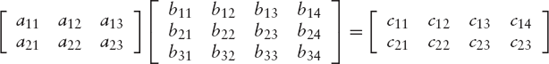
Each element cij (found in row i and column j of the product matrix C) is equal to the dot product of the ith row of A and the jth column of B. For example, to find c23, we need the numbers a21, a22 and a23 in the second row of A and b13, b23 and b33 in the third column of B. Using these two sequences as vectors, we can compute their dot product, finding
c23 = (a21, a22, a23) · (b13, b23, b33) = (a21b13 + a22b23 + a23b33)
In general, the elements of the above matrix C are computed as follows:
cij = (ai1, ai2, ai3) · (b1j, b2j, b3j) = ai1b1j + ai2b2j + ai3b3j
A transformation T is a mapping
| v → Tv = v′ |
such that each vector v (in the vector space we are dealing with) is assigned its unique image v′. Let us begin with the xy-plane and associate with each vector v the point P, such that
| v = OP |
Then the transformation T is also a mapping
| P → P′ |
for each point P in the xy-plane, where OP′ = v′.
A transformation is said to be linear if the following is true for any two vectors v and w and for any real number λ:
| T(v + w) = T(v) + T(w) |
| T(λv) = λ T(v) |
By using λ = 0 in the last equation, we find that, for any linear transformation, we have
| T(0)= 0 |
We can write any linear transformation as a matrix multiplication. For example, consider the following linear transformation:
We can write this as the matrix product
or as the following:
The notation of (3.1) is normally used in standard mathematics textbooks; in computer graphics and other applications in which transformations are combined, the notation of (3.2) is also popular because it avoids a source of mistakes, as we will see in a moment. We will therefore adopt this notation, using row vectors.
It is interesting to note that, in {(3.2)}, the rows of the 2 × 2 transformation matrix are the images of the unit vectors (1, 0) and (0, 1), respectively, while these images are the columns in (3.1). You can easily verify this by substituting [1 0] and [0 1] for [x y] in (3.2), as the bold matrix elements below illustrate:
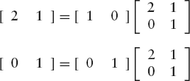
This principle also applies to other linear transformations. It provides us with a convenient way of finding the transformation matrices.
To rotate all points in the xy-plane about O through the angle φ, we can now easily write the transformation matrix, using the rule we have just been discussing. We simply find the images of the unit vectors (1, 0) and (0, 1). As we know from elementary trigonometry, rotating the points P(1, 0) and Q(0, 1) about O through the angle φ gives P′(cos φ, sin φ) and Q′(– sin φ, cos φ). It follows that (cos φ, sin φ) and (– sin φ, cos φ) are the desired images of the unit vectors (1, 0) and (0, 1), as Figure 3.1 illustrates.
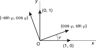
Then all we need to do is to write these two images as the rows of our rotation matrix:
To see rotation in action, let us rotate an arrow about the origin O. Before this rotation, the arrow is vertical, points upward and can be found to the right of O. We will rotate this angle through 120° about the origin O, which is the center of the canvas. Figure 3.2 shows the coordinate axes (intersecting at O) and the arrow before and after the rotation.
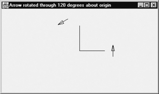
If we change the dimensions of the window, the origin remains in the center and the sizes of the arrows and of the circle on which they lie change accordingly, while this circle remains a circle. Recall that we also placed the origin at the center of the canvas in the Isotrop.java program in Section 1.4, when dealing with the isotropic mapping mode. The following program also uses this mapping mode and contains the same methods iX and iY for the conversion from logical to device coordinates:
// Arrow.java: Arrow rotated through 120 degrees about the logical
//             origin O, which is the center of the canvas.
import java.awt.*;
import java.awt.event.*;

public class Arrow extends Frame
{  public static void main(String[] args){new Arrow();}

   Arrow()
   {  super("Arrow rotated through 120 degrees about origin");
      addWindowListener(new WindowAdapter()
         {public void windowClosing(WindowEvent e){System.exit(0);}});
      setSize (400, 300);
      add("Center", new CvArrow());
      show();
   }
}
class CvArrow extends Canvas
{ int centerX, centerY, currentX, currentY;
float pixelSize, rWidth = 100.0F, rHeight = 100.0F;
void initgr()
{ Dimension d = getSize();
int maxX = d.width - 1, maxY = d.height - 1;
pixelSize = Math.max(rWidth/maxX, rHeight/maxY);
centerX = maxX/2; centerY = maxY/2;
}
int iX(float x){return Math.round(centerX + x/pixelSize);}
int iY(float y){return Math.round(centerY - y/pixelSize);}
void moveTo(float x, float y)
{ currentX = iX(x); currentY = iY(y);
}
void lineTo(Graphics g, float x, float y)
{ int x1 = iX(x), y1 = iY(y);
g.drawLine(currentX, currentY, x1, y1);
currentX = x1; currentY = y1;
}
void drawArrow(Graphics g, float[]x, float[]y)
{ moveTo(x[0], y[0]);
lineTo(g, x[1], y[1]);
lineTo(g, x[2], y[2]);
lineTo(g, x[3], y[3]);
lineTo(g, x[1], y[1]);
}
public void paint(Graphics g)
{ float r = 40.0F;
float[] x = {r, r, r-2, r+2},
y = {−7, 7, 0, 0};
initgr();
// Show coordinate axes:
moveTo (30, 0); lineTo(g, 0, 0); lineTo(g, 0, 30);
// Show initial arrow:
drawArrow(g, x, y);
float phi = (float)(2 * Math.PI / 3),
c = (float)Math.cos(phi), s = (float)Math.sin(phi),r11 = c, r12 = s, r21 = -s, r22 = c;
for (int j=0; j<4; j++)
{ float xNew = x[j] * r11 + y[j] * r21,
yNew = x[j] * r12 + y[j] * r22;
x[j] = xNew; y[j] = yNew;
}
// Arrow after rotation:
drawArrow(g, x, y);
}
}The logical coordinates of the four relevant points of the arrow are stored in the arrays x and y, and the variables r11, r12, r21 and r22 denote the elements of the rotation matrix. When programming rotations, we should be careful with two points. First, with a constant angle φ, we should compute cos φ and sin φ only once, even though they occur twice in the rotation matrix. Second, a serious and frequently occurring error is modifying x[j] too early, that is, while we still need the old value for the computation of y[j], as the following, incorrect fragment shows:
x[j] = x[j] * r11 + y[j] * r21; // ???
y[j] = x[j] * r12 + y[j] * r22;
There is no such problem if we use temporary variables xNew and yNew (although only the former is really required), as is done in the program.
Suppose that we want to perform scaling with scale factors sx for x and sy for y and with point O remaining at the same place; the latter is also expressed by referring to O as a fixed point or by a scaling with reference to O. This can obviously be written as
which can also be written as a very simple matrix multiplication:
There are some important special cases:
Consider the linear transformation given by
| (1, 0) → (1, 0) |
| (0, 1) → (a, 1) |
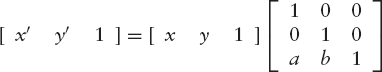
Since the images of the unit vectors appear as the rows of the transformation matrix, we can write this transformation, known as shearing, as
or
This set of equations expresses that each point (x, y) moves a distance ay to the right, which has the effect of shearing along the x-axis, as illustrated in Figure 3.3. We can use this transformation to turn regular characters into italic ones; for example, L becomes L.
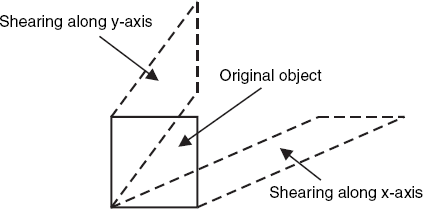
Shearing along the y-axis, also depicted in Figure 3.3, can be similarly expressed as
or
Shifting all points in the xy-plane a constant distance in a fixed direction is referred to as a translation. This is another transformation, which we can write as:
| x′ = x + a |
| y′ = y + b |
We refer to the number pair (a, b) as the shift vector, or translation vector. Although this transformation is a very simple one, it is not linear, as we can easily see by the fact that the image of the origin (0, 0) is (a, b), while this can only be the origin itself with linear transformations. Consequently, we cannot obtain the image (x′, y′) by multiplying (x, y) by a 2 × 2 transformation matrix T, which prevents us from combining such a matrix with other transformation matrices to obtain composite transformations. Fortunately, there is a solution to this problem as described in the following section.
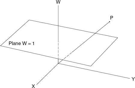
To express all the transformations introduced so far as matrix multiplications in order to combine various transformation effects, we add one more dimension. As illustrated in Figure 3.4, the extra dimension W makes any point P = (x, y) of normal coordinates have a whole family of homogeneous coordinate representations (wx, wy, w) for any value of w except 0. For example, (3, 6, 1), (0.3, 0.6, 0.1), (6, 12, 2), (12, 24, 4) and so on, represent the same point in two-dimensional space. Similarly, 4-tuples of coordinates represent points in three-dimensional space. When a point is mapped onto the W = 1 plane, in the form (x, y, 1), it is said to be homogenized. In the above example, point (3, 6, 1) is homogenized, and the numbers 3, 6 and 1 are homogeneous coordinates. In general, to convert a point from normal coordinates to homogeneous coordinates, add a new dimension to the right with value 1. To convert a point from homogeneous coordinates to normal coordinates, divide all the dimension values by the rightmost dimension value, and then discard the rightmost dimension.
Having introduced homogeneous coordinates, we are able to describe a translation by a matrix multiplication using a 3 × 3 instead of a 2 × 2 matrix. Using a shift vector (a, b), we can write the translation of Section 3.3 as the following matrix product:
Since we cannot multiply a 3 × 3 by a 2 × 2 matrix, we will also add a row and a column to linear transformation matrices if we want to combine these with translations (and possibly with other non-linear transformations). These additional rows and columns simply consist of zeros followed by a one at the end. For example, we can use the following equation instead of 3.3 (in Section 3.2) for a rotation about O through the angle φ:
A linear transformation may or may not be reversible. For example, if we perform a rotation about the origin through an angle φ and follow this by another rotation, also about the origin but through the angle -φ, these two transformations cancel each other out. Let us denote the rotation matrix of Equation (3.3) (in Section 3.2) by R. It follows that the inverse rotation, through the angle -φ instead of φ, is described by the equation
[ x′ y′ ] = [ x y ] R−1
where
The second equality in this equation is based on
| cos - φ = cos φ |
| sin − φ = - sin φ |
Matrix R−1 is referred to as the inverse of matrix R. In general, if a matrix A has an inverse, this is written A−1 and we have
| AA−1 = A−1 A = I |
where I is the identity matrix, consisting of zero elements except for the main diagonal, which contains elements one. For example, in the case of a rotation through φ, followed by one through -φ, we have
The identity matrix clearly maps each point to itself, that is,
| [x y]I = [x y] |
Not all linear transformations are reversible. For example, the one that projects each point onto the x-axis is not. This transformation is described by
which we can also write as
The 2 × 2 matrix in this equation has no inverse. This corresponds to the impossibility of reversing the linear transformation in question: since any two point P1(x, y1) and P2(x, y2) have the same image P′(x, 0), it is impossible to find a unique point P of which P′ is the image.
A (square) matrix has an inverse if and only if its determinant is non-zero. Recall that we have discussed determinants in Section 2.3. For example, the determinant
is equal to cos φ × cos φ - (- sin φ × sin φ) = cos2 φ + sin2 φ = 1. Since this value is non-zero for any angle φ, the corresponding matrix
has an inverse.
Exercise 3.4 shows how to compute the inverse of any 2 × 2 matrix that has a non-zero determinant. A useful application of this follows in Exercise 3.5.
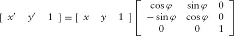
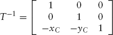
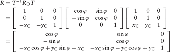
So far we have only performed rotations about the origin O. A rotation about any point other than O is not a linear transformation, since it does not map the origin onto itself. It can nevertheless be described by a matrix multiplication, provided we use homogeneous coordinates. A rotation about the point C(xC, yC) through the angle φ can be performed in three steps:
A translation from C to O, described by [x′ y′ 1] = [x y 1]T−1, where
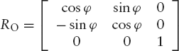
A rotation about O through the angle φ described by [x′ y′ 1] = [x y 1] RO, where
A translation from O to C, described by [x′ y′ 1] = [x y 1]T, where
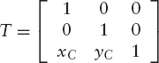
Note that we deliberately use the notations T−1 and T, since these two matrices are each other's inverse. This is understandable, since the operations of translating from C to O and then back from O to C cancel each other out.
The purpose of listing the above three matrices is that we can combine them by forming their product. Therefore, the desired rotation about point C through the angle φ can be described by
| [x′ y′ 1] = [x y 1]R |
where
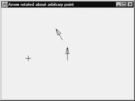
To see this general type of rotation in action, we will now discuss a program which rotates an arrow through 30° about a point selected by the user. Initially, one arrow, pointing vertically upward, appears in the center of the canvas. As soon as the user clicks a mouse button, a second arrow appears. This is the image of the first one, resulting from a rotation through an angle of 30° about the cursor position. This position is displayed as a crosshair cursor in Figure 3.5.
This action can be done repeatedly, in such a way that the most recently rotated arrow is again rotated when the user clicks, and this last rotation is performed about the most recently selected point. Since the rotation is counter-clockwise, the new arrow would have appeared below the old one in Figure 3.5 if the user had selected a point to the right instead of to the left of the first arrow. Program ArrowPt.java shows how this rotation is computed.
// ArrowPt.java: Arrow rotated through 30 degrees
//    about a point selected by the user.
import java.awt.*;
import java.awt.event.*;

public class ArrowPt extends Frame
{  public static void main(String[] args){new ArrowPt();}
ArrowPt()
{ super("Arrow rotated about arbitrary point");
addWindowListener(new WindowAdapter()
{public void windowClosing(WindowEvent e){System.exit(0);}});
setSize (400, 300);
add("Center", new CvArrowPt());
setCursor(Cursor.getPredefinedCursor(Cursor.CROSSHAIR_CURSOR));
show();
}
}
class CvArrowPt extends Canvas
{ int centerX, centerY, currentX, currentY;
float pixelSize, xP = 1e9F, yP,
rWidth = 100.0F, rHeight = 100.0F;
float[] x = {0, 0, −2, 2}, y = {−7, 7, 0, 0};
CvArrowPt()
{ addMouseListener(new MouseAdapter()
{ public void mousePressed(MouseEvent evt)
{ xP = fx(evt.getX()); yP = fy(evt.getY());
repaint();
}
});
}
void initgr()
{ Dimension d = getSize();
int maxX = d.width - 1, maxY = d.height - 1;
pixelSize = Math.max(rWidth/maxX, rHeight/maxY);
centerX = maxX/2; centerY = maxY/2;
}
int iX(float x){return Math.round(centerX + x/pixelSize);}
int iY(float y){return Math.round(centerY - y/pixelSize);}
float fx(int x){return (x - centerX) * pixelSize;}
float fy(int y){return (centerY - y) * pixelSize;}
void moveTo(float x, float y)
{ currentX = iX(x); currentY = iY(y);
}void lineTo(Graphics g, float x, float y)
{ int x1 = iX(x), y1 = iY(y);
g.drawLine(currentX, currentY, x1, y1);
currentX = x1; currentY = y1;
}
void drawArrow(Graphics g, float[]x, float[]y)
{ moveTo(x[0], y[0]);
lineTo(g, x[1], y[1]);
lineTo(g, x[2], y[2]);
lineTo(g, x[3], y[3]);
lineTo(g, x[1], y[1]);
}
public void paint(Graphics g)
{ initgr();
// Show initial arrow:
drawArrow(g, x, y);
if (xP > 1e8F) return;
float phi = (float)(Math.PI / 6),
c = (float)Math.cos(phi), s = (float)Math.sin(phi),
r11 = c, r12 = s,
r21 = -s, r22 = c,
r31 = -xP * c + yP * s + xP, r32 = -xP * s - yP * c + yP;
for (int j=0; j<4; j++)
{ float xNew = x[j] * r11 + y[j] * r21 + r31,
yNew = x[j] * r12 + y[j] * r22 + r32;
x[j] = xNew; y[j] = yNew;
}
// Arrow after rotation:
drawArrow(g, x, y);
}
}In contrast to program Arrow.java of Section 3.2, this new program ArrowPt.java uses the 3 × 3 rotation matrix displayed in Equation (3.6), as you can see in the fragment
float xNew = x[j] * r11 + y[j] * r21 + r31,
      yNew = x[j] * r12 + y[j] * r22 + r32;
The matrix elements r31 and r32 of the third row of the matrix depend on the point (xP, yP), selected by the user and acting as the center C(xC, yC) in our previous discussion. As in program Isotrop.java of Section 1.4, the device coordinates of the selected point P are converted to logical coordinates by the methods fx and fy.
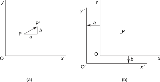
In the preceding sections, we have used a fixed coordinate system and applied transformations to points given by their coordinates for that system, using certain computations. We can use exactly the same computations for a different purpose, leaving the points unchanged but changing the coordinate system. It is important to bear in mind that the direction in which the coordinate system moves is opposite to that of the point movement. We can see this very clearly in the case of a translation. In Figure 3.6(a) we have a normal translation with any point P(x, y) mapped to its image P′(x′, y′), where
| x′ = x + a |
| y′ = y + b |
which can be written in matrix form as shown in Equation (3.4) (in Section 3.4). In Figure 3.6(b) we do not map the point P to another point but we express the position of this point in the x′y′-coordinate system, while coordinates x and y are given. As you can see, a translation upward and to the right in (a), corresponds with a movement of the coordinate system downward and to the left in (b): these two directions are exactly each other's opposite. It follows that the inverse translation matrix would have applied if, in (b), we had moved the axes in the same direction as that of the point translation. The same principle applies to other transformations, such as rotations, for which the inverse of the transformation matrix exists. We will use this principle in the next section.
Let us use a right-handed three-dimensional coordinate system, with the positive x-axis pointing toward us, the y-axis pointing to the right and the z-axis pointing upward, as shown in Figure 3.7.
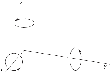
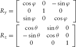
This figure also shows what we mean by rotations about the axes. A rotation about the z-axis through a given angle implies a rotation of all points in the xy-plane through that angle. For example, if this angle is 90°, the image of all points of the positive x-axis will be those of the positive y-axis. In the same way, a rotation about the x-axis implies a similar rotation of the yz-plane and a rotation about the y-axis implies a similar rotation of the zx-plane. Note that we deliberately write zx in that order: when we are dealing with the x-, y- and z-axes in a cyclic way, x follows z. It is important to remember this when we have to write down the transformation matrices for the rotations about the x-, y- and z-axis through the angle φ:
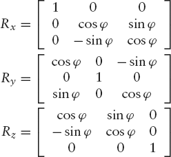
These matrices are easy to construct. Matrix Rz is derived in a trivial way from the well-known 2 × 2 rotation matrix of Equation (3.3) (in Section 3.2). If you check this carefully, you will not find the other two matrices difficult. First, there is a 1 on the main diagonal in the position that corresponds to the axis of rotation (1 for x, 2 for y and 3 for z). The other elements in the same row or column as this matrix element 1 are equal to 0. Second, we use the elements of the 2 × 2 matrix just mentioned for the remaining elements of the 3 × 3 matrices, beginning just to the right and below the element 1, if that is possible; if not, we remember that x follows z. For example, in Ry, the first element, cos φ, of this imaginary 2 × 2 matrix is placed in row 3 and column 3 because the element 1 has been placed in row 2 and column 2. Then, since we cannot place sin φ to the right of this element cos φ as we would like, we place it instead in column 1 of the same third row. In the same way, we cannot place – sin φ below cos φ, as it occurs in Equation (3.3), so instead we put it in the first row of the same third column, and so on.
We should remember that the above matrices should be applied to row vectors. For example, using the above matrix Rx, we write
| [x′ y′ z′] = [x y z] Rx |
to obtain the image (x′, y′, z′) of point (x, y, z) when the latter is subjected to a rotation about the x-axis through an angle φ.
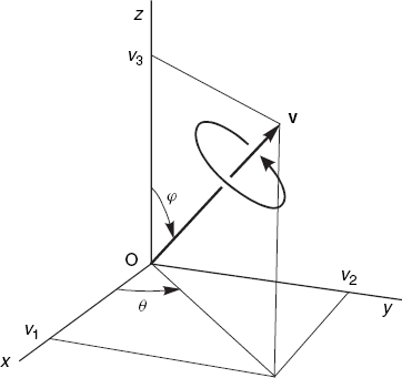
To prepare for a three-dimensional rotation about an arbitrary axis, let us first perform such a rotation about an axis through the origin O. Actually, the rotation will take place about a vector, so that we can define its orientation, as illustrated by Figure 3.8.
If a point is rotated about the vector v through a positive angle α, this rotation will be such that it corresponds to a movement in the direction of the vector in the same way as turning a (right-handed) screw corresponds to its forward movement.
Instead of its Cartesian coordinates (v1, v2, v3), we will use the angles θ and φ to specify the direction of the vector v. The length of this vector is irrelevant to our present purpose. As you can see in Figure 3.8, θ is the angle between the positive x-axis and the projection of v in the xy-plane and φ is the angle between the positive z-axis and the vector v. If v1, v2 and v3 are given and we want to find {θ} and φ, we can compute them in Java in the following way, writing theta for {θ} and phi for φ:
theta = Math.atan2(v2, v1);
phi = Math.atan2(Math.sqrt(v1 * v1 + v2 * v2), v3);
We will now derive a rather complicated 3 × 3 rotation matrix, which describes the rotation about the vector v through an angle α. First, we will change the coordinate system such that v will lie on the positive z-axis. This can be done in two steps:
A rotation of the coordinate system about the z-axis, such that the horizontal component of v lies on the new x-axis.
A rotation of the coordinate system about the new y-axis though the angle φ.
As discussed at the end of the previous section, coordinate transformations require the inverses of the matrices that we would use for normal rotations of points. Referring to Section 3.8, we now have to use the following matrices Rz−1 and Ry−1 for the above steps 1 and 2, respectively:
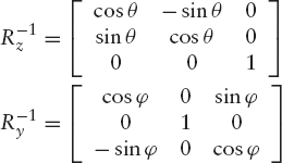
To combine these two coordinate transformations, we have to use the product of these two matrices. Before doing this matrix multiplication, let us first find the matrices of some more operations that are required.
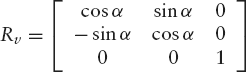
Now that the new positive z-axis has the same direction as the vector v, the desired rotation about v through the angle α is also a rotation about the z-axis through that angle, so that, expressed in the new coordinates, we have the following rotation matrix:
Although this may seem to be the final operation, we must bear in mind that we want to express the image point P′ of an original point P in terms of the original coordinate system. This implies that the first two of the above three transformations are to be followed by their inverse transformations, in reverse order. Therefore, in this order, we have to use the following two matrices after the three above:
The resulting matrix R, to be used in the equation
| [x′ y′ z′] = [x y z]R |
to perform a rotation about v through the angle α, can now be found as follows:
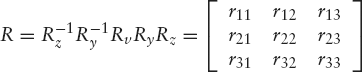
where the matrix elements rij are rather complicated expressions in φ, θ and α. Before discussing how to compute these, let us first turn to the original problem, which was the same as the above, except that we want to use any point A(a1, a2, a3) as the start point of vector v. We can do this by performing, in this order:
a translation that shifts the point A to the origin O;
the desired rotation using the above matrix R;
the inverse of the translation just mentioned.
As discussed in Sections 3.4 and 3.6, we need to use homogeneous coordinates in order to describe translations by matrix multiplications. Since we use 3 × 3 matrices for linear transformations in three-dimensional space, we have to use 4 × 4 matrices in connection with these homogenous coordinates. Based on the coordinates a1, a2 and a3 of the point A on the axis of rotation, the following matrix describes the translation from A to O:
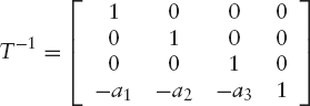
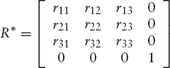
After this translation, we perform the rotation about the vector v, which starts at point A, using the above matrix R, which we write as R* after adding an additional row and column in the usual way:
Finally, we use a translation from O back to A:
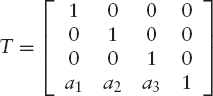
Writing RGEN for the desired general (4 × 4) rotation matrix, we have
| RGEN = T−1R*T |
Since RGEN is a 4 × 4 matrix, we use it as follows:
| [x′ y′ z′ 1] = [x y z 1] RGEN |
Since we are now dealing with points in three-dimensional space, let us begin by defining the following class to represent such points:
// Point3D.java: Representation of a point in 3D space.
class Point3D
{  float x, y, z;
   Point3D(double x, double y, double z)
   {  this.x = (float)x;
      this.y = (float)y;
      this.z = (float)z;
   }
}
As we normally have a great many points that are to be rotated, it is worthwhile to compute the matrix RGEN beforehand. Although this could be done numerically, it is also possible to make our program slightly faster by doing this symbolically, that is, by expressing all matrix elements rij of RGEN in six constant values for the rotation: the angles φ, θ and α and the coordinates a1, a2 and a3 of point A on the axis of rotation. Instead of writing these matrix elements here in the usual mathematical formulas (which would be quite complicated), we may as well immediately present the resulting Java code. This has been done in the class Rotate3D below.
The actual rotation is performed by the rotate method, which is called as many times as there are relevant points (usually the vertices of polyhedra). Prior to this, the method initRotate is called only once, to build the above matrix RGEN. There are actually two methods initRotate, of which we can choose one as we like. The first accepts two points A and B to specify the directed axis of rotation AB and computes the angles {θ} and φ. The second accepts these two angles themselves instead of point B:
// Rota3D.java: Class used in other program files
//    for rotations about an arbitrary axis.
// Uses: Point3D (discussed above).
class Rota3D
{  static double r11, r12, r13, r21, r22, r23,
                 r31, r32, r33, r41, r42, r43;

/* The method initRotate computes the general rotation matrix

            | r11  r12  r13  0 |
       R =  | r21  r22  r23  0 |
            | r31  r32  r33  0 |
            | r41  r42  r43  1 |

   to be used as [x1  y1  z1  1] = [x  y  z  1] R
   by the method 'rotate'.
   Point (x1, y1, z1) is the image of (x, y, z).
   The rotation takes place about the directed axis
   AB and through the angle alpha.
*/
   static void initRotate(Point3D a, Point3D b,
      double alpha)
   {  double v1 = b.x - a.x,
             v2 = b.y - a.y,
             v3 = b.z - a.z,
         theta = Math.atan2(v2, v1),
         phi = Math.atan2(Math.sqrt(v1 * v1 + v2 * v2), v3);
initRotate(a, theta, phi, alpha);
}
static void initRotate(Point3D a, double theta,
double phi, double alpha)
{ double cosAlpha, sinAlpha, cosPhi, sinPhi,
cosTheta, sinTheta, cosPhi2, sinPhi2,
cosTheta2, sinTheta2, pi, c,
a1 = a.x, a2 = a.y, a3 = a.z;
cosPhi = Math.cos(phi); sinPhi = Math.sin(phi);
cosPhi2 = cosPhi * cosPhi; sinPhi2 = sinPhi * sinPhi;
cosTheta = Math.cos(theta);
sinTheta = Math.sin(theta);
cosTheta2 = cosTheta * cosTheta;
sinTheta2 = sinTheta * sinTheta;
cosAlpha = Math.cos(alpha);
sinAlpha = Math.sin(alpha);
c = 1.0 - cosAlpha;
r11 = cosTheta2 * (cosAlpha * cosPhi2 + sinPhi2)
+ cosAlpha * sinTheta2;
r12 = sinAlpha * cosPhi + c * sinPhi2 * cosTheta * sinTheta;
r13 = sinPhi * (cosPhi * cosTheta * c - sinAlpha * sinTheta);
r21 = sinPhi2 * cosTheta * sinTheta * c - sinAlpha * cosPhi;
r22 = sinTheta2 * (cosAlpha * cosPhi2 + sinPhi2)
+ cosAlpha * cosTheta2;
r23 = sinPhi * (cosPhi * sinTheta * c + sinAlpha * cosTheta);
r31 = sinPhi * (cosPhi * cosTheta * c + sinAlpha * sinTheta);
r32 = sinPhi * (cosPhi * sinTheta * c - sinAlpha * cosTheta);
r33 = cosAlpha * sinPhi2 + cosPhi2;
r41 = a1 - a1 * r11 - a2 * r21 - a3 * r31;
r42 = a2 - a1 * r12 - a2 * r22 - a3 * r32;
r43 = a3 - a1 * r13 - a2 * r23 - a3 * r33;
}
static Point3D rotate(Point3D p)
{ return new Point3D(
p.x * r11 + p.y * r21 + p.z * r31 + r41,
p.x * r12 + p.y * r22 + p.z * r32 + r42,
p.x * r13 + p.y * r23 + p.z * r33 + r43);
}
}Note that the actual rotation of points is done very efficiently in the method rotate at the end of this class. This is important because it will be called for each relevant point of the object to be rotated. Remember, the more time-consuming method initRotate is called only once.
Let us now see this class Rota3D in action. Although it can be used for any rotation axis and any angle of rotation, it is used here only in a very simple way so that we can easily check the result, even without graphics output. As Figure 3.9 shows, we have chosen the axis AB parallel to the diagonals 0–2 and 4–6 of the cube. The cube has a height 1 and point A has coordinates (0, 0, 2).
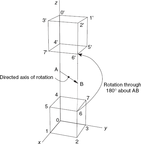
The following program uses the above classes Point3D and Rota3D to perform the rotation shown in Figure 3.9:
// Rota3DTest.java: Rotating a cube about an axis
//    parallel to a diagonal of its top plane.
//    Uses: Point3D, Rota3D (discussed above).
public class Rota3DTest
{  public static void main(String[] args)
{ Point3D a = new Point3D (0, 0, 1), b = new Point3D (1, 1, 1);
double alpha = Math.PI;
// Specify AB as directed axis of rotation
// and alpha as the rotation angle:
Rota3D.initRotate(a, b, alpha);
// Vertices of a cube; 0, 1, 2, 3 at the bottom,
// 4, 5, 6, 7 at the top. Vertex 0 at the origin O:
Point3D[] v = {
new Point3D (0, 0, 0), new Point3D (1, 0, 0),
new Point3D (1, 1, 0), new Point3D (0, 1, 0),
new Point3D (0, 0, 1), new Point3D (1, 0, 1),
new Point3D (1, 1, 1), new Point3D (0, 1, 1)};
System.out.println(
"Cube rotated through 180 degrees about line AB,");
System.out.println(
"where A = (0, 0, 1) and B = (1, 1, 1) ");
System.out.println("Vertices of cube:");
System.out.println(
" Before rotation After rotation");
for (int i=0; i<8; i++)
{ Point3D p = v[i];
// Compute P1, the result of rotating P:
Point3D p1 = Rota3D.rotate(p);
System.out.println(i + ": " +
p.x + " " + p.y + " " + p.z + " " +
f(p1.x) + " " + f(p1.y) + " " + f(p1.z));
}
}
static double f(double x){return Math.abs(x) < 1e-10 ? 0.0 : x;}
}Since we have not yet discussed how to produce perspective views, we produce only text output in this program, as listed below:
Cube rotated through 180 degrees about line AB,
where A =  (0, 0, 2)  and B =  (1, 1, 2)
Vertices of cube:
    Before rotation    After rotation
0:  0.0 0.0 0.0        0.0 0.0 4.0
1:  1.0 0.0 0.0        0.0 1.0 4.0
2:  1.0 1.0 0.0        1.0 1.0 4.0
3:  0.0 1.0 0.0        1.0 0.0 4.0
4: 0.0 0.0 1.0 0.0 0.0 3.0 5: 1.0 0.0 1.0 0.0 1.0 3.0 6: 1.0 1.0 1.0 1.0 1.0 3.0 7: 0.0 1.0 1.0 1.0 0.0 3.0
EXERCISES
3.1 In Section 3.2 we discussed scaling with reference to the origin O, that is, with O as a fixed point. It is also possible to use a different fixed point, say C(xC, yC), but, for such a scaling in two-dimensional space, we need a 3 × 3 matrix M (and homogenous coordinates), writing
| [x′ y′ 1] = [x y 1]M |
Using scale factors sx and sy for x and y again, find this matrix M.
Hint: You can perform a translation from C to O, followed by a scaling as discussed in Section 3.2, but described by a 3 × 3 matrix, followed by a translation back from O to C. Alternatively, you can start with the following system of equations, which shows very clearly what actually happens:
3.2 Describe scaling in three-dimensional space with reference to a point C and three scale factors sx, sy and sz. Find the 4 × 4 matrix (similar to matrix M of Exercise 3.1) for this transformation.
3.3 How can you apply shearing with reference to a point other than O (such that this point will remain at the same place)? Write a program that draws a square and an approximate circle, both before and after shearing, setting the constant a used at the end of Section 3.2 equal to 0.5. Apply shearing to these two figures with reference to their centers; in other words, the center of the square will remain at the same place and so will the center of the circle.
3.4 (This exercise prepares for the next one.) If the determinant D = a11a22 - a12a21 of the matrix
is non-zero, then the matrix
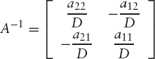
is the inverse of A, that is,
3.5 Our way of testing whether a given point P lies in a triangle ABC, discussed in Section 2.8, resulted in the method insideTriangle, which assumes that A, B and C are counter-clockwise. Develop a different method for the same purpose, based on the vectors a = (a1, a2) = CA and b = (b1, b2) = CB (see Figure 2.6 in Section 2.5). Let us write
CP = p = (p1, p2) = λa + μb
or, in the form of a matrix product,
Since we saw in Exercise 3.4 how to compute the inverse of a 2 × 2 matrix, we can now compute λ and μ as follows:
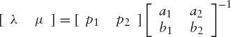
The point P lies in triangle ABC (or on one of its edges) if and only if λ ≥ 0, μ ≥ 0 and λ + μ ≤ 1. Write the class TriaTest, which we can use as follows:
Point2D a, b, c, p;
TriaTest tt = new TriaTest(a, b, c);
if (tt.area2() != 0 && tt.insideTriangle(p)) ...
   // Point P within triangle ABC.
As in Section 2.5, the method area2 returns twice the area of triangle ABC, preceded by a minus sign if ABC is clockwise. This return value is also equal to the determinant of the 2 × 2 matrix in Equation (3.7). We must not call the TriaTest method insideTriangle if this determinant is zero, since in that case the inverse matrix of Equation (3.8) does not exist (see Exercise 3.4).