Although programming is a very creative activity, often requiring entirely new (little) problems to be solved, we can sometimes benefit from well-known algorithms, published by others and usually providing more efficient or more elegant solutions than those we would have been able to invent ourselves. This is no different in computer graphics. This chapter is about some well-known graphics algorithms for (a) computing the coordinates of pixels that comprise lines and circles, (b) clipping lines and polygons, and (c) drawing smooth curves. These are the most primitive operations in computer graphics and should be executed as fast as possible. Therefore, the algorithms in this chapter ought to be optimized to avoid time-consuming executions, such as multiplication, division, and calculations on floating point numbers.
We will now discuss how to draw lines by placing pixels on the screen. Although, in Java, we can simply use the method drawLine without bothering about pixels, it would be unsatisfactory if we had no idea how this method works. We will be using integer coordinates, but when discussing the slope of a line it would be very inconvenient if we had to use a y-axis pointing downward, as is the case with the Java device coordinate system. Therefore, in accordance with mathematical usage, the positive y-axis will point upward in our discussion.
Unfortunately, Java lacks a method with the sole purpose of putting a pixel on the screen, so that we define the following, rather strange method to achieve this:
void putPixel(Graphics g, int x, int y)
{  g.drawLine(x, y, x, y);
}
We will now develop a drawLine method of the form
void drawLine(Graphics g, int xP, int yP, int xQ, int yQ)
{ ...
}
which only uses the above putPixel method for the actual graphics output.
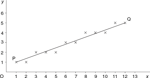
Figure 4.1 shows a line segment with endpoints P(1, 1) and Q(12, 5), as well as the pixels that we have to compute to approximate this line.
To draw the line of Figure 4.1, we then write
drawLine(g, 1, 1, 12, 5);
Let us first solve the problem for situations such as Figure 4.1, in which point Q lies to the right and not lower than point P. More precisely, we will be dealing with the special case
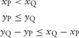
where the last condition expresses that the angle of inclination of line PQ is not greater than 45°. We then want to find exactly one integer y for each of the integers
| xp, xp + 1, xp + 2, . . . , xQ |
Except for the first and the last (which are given as yp and yQ) the most straightforward way of computing these y-coordinates is by using the slope
so that, for each of the given integer x-coordinates, we can find the desired integer y-coordinate by rounding the value
| yexact = yP + m(x - xP) |
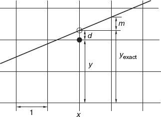
to the nearest integer. Since two such successive x-coordinates differ by 1, the corresponding difference of two successive values of yexact is equal to m. Figure 4.2 shows this interpretation of m, as well as that of the 'error'
Since d is the error we make by rounding yexact to the nearest integer, we can require d to satisfy the following condition:
The following first version of the desired drawLine method is based on this observation:
void drawLine1(Graphics g, int xP, int yP, int xQ, int yQ)
{  int x = xP, y = yP;
   float d = 0, m = (float)(yQ - yP)/(float)(xQ - xP);
for (;;)
{ putPixel(g, x, y);
if (x == xQ) break;
x++;
d += m;
if (d >= 0.5){y++; d--;}
}
}This version is easy to understand if we pay attention to Figure 4.2. Since the first call to putPixel applies to point P, we begin with the error d = 0. In each step of the loop, x is increased by 1. Assuming for the moment that y will not change, it follows from Equation (4.3) that the growth of d will be the same as that of yexact, which explains why d is increased by m. We then check the validity of this assumption in the following if-statement. If d is no longer less than 0.5, this violates Equation (4.4), so that we apply a correction, consisting of increasing y and decreasing d by 1. The latter action makes Equation (4.4) valid again. By doing these two actions at the same time, Equation (4.3) also remains valid.
We use drawLine1 as a basis for writing a faster version, which no longer uses type float. This is possible because the slope variable m represents a rational number, that is, an integer numerator divided by an integer denominator, as Equation (4.2) shows. Since the other float variable, d, starts with the value zero and is altered only by adding m and −1 to it, it is also a rational number. In view of both the denominator xQ – xP of these rational numbers and the constant 0.5 used in the if-statement, we will apply the scaling factor
| c = 2 (xQ – xp) |
to m, to d and to this constant 0.5, introducing the int variables M and D instead of the float variables m and d. We will also use Δx instead of the constant 0.5.
These new values M, D and Δx are c times as large as m, d and 0.5, respectively:
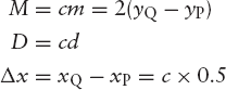
In this way we obtain the following integer version, which is very similar to the previous one and equivalent to it but faster. In accordance with the Java naming conventions for variables, we write m and d again instead of M and D, and dx instead of Δx:
void drawLine2(Graphics g, int xP, int yP, int xQ, int yQ)
{  int x = xP, y = yP, d = 0, dx = xQ - xP, c = 2 * dx,
      m = 2 * (yQ - yP);
   for (;;)
   {  putPixel(g, x, y);
      if (x == xQ) break;
      x++;
      d += m;
      if (d >= dx){y++; d -= c;}
   }
}
Having dealt with this special case, with points P and Q satisfying Equation (4.1), we now turn to the general problem, without any restrictions with regard to the relative positions of P and Q. To solve this, we have several symmetric cases to consider. As long as
| |yQ – yP| ≤ |xQ – xP| |
we can again use x as the independent variable, that is, we can increase or decrease this variable by one in each step of the loop. In the opposite case, with lines that have an angle of inclination greater than 45°, we have to interchange the roles of x and y to prevent the selected pixels from lying too far apart. All this is realized in the general line-drawing method drawLine below. We can easily verify that this version plots exactly the same points approximating line PQ as version drawLine2 if the coordinates of P and Q satisfy Equation (4.1).
void drawLine(Graphics g, int xP, int yP, int xQ, int yQ)
{  int x = xP, y = yP, d = 0, dx = xQ - xP, dy = yQ - yP,
      c, m, xInc = 1, yInc = 1;
   if (dx < 0){xInc = −1; dx = -dx;}
   if (dy < 0){yInc = −1; dy = -dy;}
   if (dy <= dx)
   {  c = 2 * dx; m = 2 * dy;
if (xInc < 0) dx++;
for (;;)
{ putPixel(g, x, y);
if (x == xQ) break;
x += xInc;
d += m;
if (d >= dx){y += yInc; d -= c;}
}
}
else
{ c = 2 * dy; m = 2 * dx;
if (yInc < 0) dy++;
for (;;)
{ putPixel(g, x, y);
if (y == yQ) break;
y += yInc;
d += m;
if (d >= dy){x += xInc; d -= c;}
}
}
}Just before executing one of the above two for-statements, an if-statement is executed in the cases that x or y decreases instead of increases, which is required to guarantee that drawing PQ always plots exactly the same points as drawing QP.
The idea of drawing sloping lines by means of only integer variables was first realized by Bresenham; his name is therefore associated with this algorithm.
The above drawLine method is very easy to use if we are dealing with the floating-point logical-coordinate system used so far. For example, in Section 4.5, there will be a program ClipPoly.java, in which the following method occurs:
void drawLine(Graphics g, float xP, float yP, float xQ, float yQ)
{  g.drawLine(iX(xP), iY(yP), iX(xQ), iY(yQ));
}
Here our own method drawLine calls the Java method drawLine of the class Graphics. If, instead, we want to use our own method drawLine with four int arguments, listed above, we can replace the last three program lines with
void drawLine(Graphics g, float xP, float yP, float xQ, float yQ)
{  drawLine(g, iX(xP), iY(yP), iX(xQ), iY(yQ)); // int coordinates
}
provided that we also add the method putPixel, listed at the beginning of this section. This may at first be confusing because there are now two drawLine methods of our own. As the comment after the above call to drawLine indicates, the Java compiler will select our Bresenham method drawLine because there is an argument g, followed by four arguments of type int. It is also interesting to note that the direction of the positive y-axis in our discussion causes no practical problem.
As one of the primitive graphics operations, line drawing should be performed as rapidly as possible. In fact, graphics hardware is typically benchmarked by the speed in which it generates lines. Bresenham's line algorithm is simple and efficient in generating lines. The algorithm works incrementally by computing the position of the next pixel to be drawn. Hence it iterates as many times as the number of pixels in the line it generates. The double-step line-drawing algorithm by Rokne, Wyvill, and Wu (1990) aims at reducing the number of iterations by half, by computing the positions of the next two pixels.
Let us again start with the lines within the slope range of [0, 1] and consider the general case of any slopes later (as Exercise 4.2). For a line PQ, starting from P, we increment the x-coordinate by two pixels instead of one as in Bresenham's algorithm. All the possible positions of the two pixels in the above slope range form four patterns, expressed in a 2×2 mesh illustrated in Figure 4.3. It has been mathematically proven that patterns 1 and 4 would never occur on the same line, implying that a line would possibly involve patterns 1, 2 and 3, or patterns 2, 3 and 4, depending the slope of the line. The lines within the slope range of [0, 1/2) involve patterns 1, 2 and 3, and lines within the slope range of (1/2, 1] involve patterns 2, 3 and 4. At the exact slope of 1/2, the line involves either pattern 2 or 3, not 1 or 4.
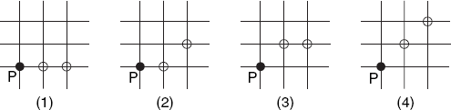
Figure 4.4 shows four sloping lines, all passing through the same point at a distance d above the point A. By approximating this common point of the four lines we make an error d = yexact–y, which should not be greater than 0.5.
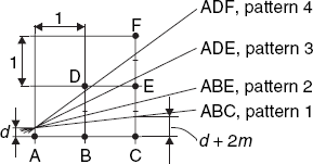
Since the slope of a line is equal to m, the exact y-coordinate of that line is equal to d + m at its point of intersection with BD, and d + 2m at its point of intersection with CF, as indicated in Figure 4.4 for the lowest of the four lines. With these two points of intersection lying closer to BC than to DE, it is clear that this lowest sloping line should be approximated by the points A, B, C, that is, by pattern 1 of Figure 4.3. Thus we have
| if d + 2m < 0.5, we use pattern 1(ABC) |
Otherwise, we use point E instead of C if E is the best approximation of the point where the sloping line intersects CF, that is, if 0.5 ≤ d + 2m ≤ 1.5. However, we should now also pay attention to the point where the sloping line intersects BD. Comparing d + m with 0.5 determines whether B or D should be taken. More precisely,
| if 0.5 ≤ d + 2m < 1.5 (so that point E is to be used), we choose B or D as follows: |
| if d + m < 0.5, we use pattern 2(ABE) |
| if d + m ≥ 0.5, we use pattern 3(ADE) |
Finally, there is this remaining case:
| if d + 2m ≥ 1.5, we use pattern 4(ADF). |
As in the previous section when discussing Bresenham's algorithm, we begin with a preliminary method that still uses floating-point variables to make it easier to understand, so it is not yet optimized for speed. This version also works for lines drawn from right to left, that is, when xQ < xP, as well as for lines with negative slope. However, the absolute value of the slope should not be greater than 1. So doubleStep1 applies only to endpoints P and Q that satisfy the following conditions:
| xQ ≠ xP |
| |yQ – yP| ≤ |xQ – xP| |
It is wise to begin with the simplest case
| xP < xQ |
| 0 ≤ yQ – yP ≤ xQ – xP |
when you read the following code for the first time:
void doubleStep1(Graphics g, int xP, int yP, int xQ, int yQ)
{  int dx, dy, x, y, yInc;
   if (xP >= xQ)
   {  if (xP == xQ) // Not allowed because we divide by dx (= xQ - xP)
         return;
      // xP > xQ, so swap the points P and Q
      int t;
      t = xP; xP = xQ; xQ = t;
      t = yP; yP = yQ; yQ = t;
   }
   // Now xP < xQ
   if (yQ >= yP){yInc = 1; dy = yQ - yP;}  // Normal case, yP < yQ
   else         {yInc = −1; dy = yP - yQ;}
   dx = xQ - xP;  // dx > 0, dy > 0
   float d = 0,                   // Error d = yexact - y
         m = (float)dy/(float)dx; //  m <= 1, m = | slope |
   putPixel(g, xP, yP);
   y = yP;
   for (x=xP; x<xQ-1;)
   {  if (d + 2 * m < 0.5) // Pattern 1:
      {  putPixel(g, ++x, y);
         putPixel(g, ++x, y);
         d += 2 * m; // Error increases by 2m, since y remains
                     // unchanged and yexact increases by 2m
      }
      else
      if (d + 2 * m < 1.5) // Pattern 2 or 3
      {  if (d + m < 0.5)  // Pattern 2
         {  putPixel(g, ++x, y);
            putPixel(g, ++x, y += yInc);
            d += 2 * m − 1; // Because of ++y, the error is now
                            // 1 less than with pattern 1
         }
         else  // Pattern 3
         {  putPixel(g, ++x, y += yInc);
            putPixel(g, ++x, y);
            d += 2 * m − 1;  // Same as pattern 2
}
}
else // Pattern 4:
{ putPixel(g, ++x, y += yInc);
putPixel(g, ++x, y += yInc);
d += 2 * m − 2; // Because of y += 2, the error is now
// 2 less than with pattern 1
}
}
if (x < xQ) // x = xQ - 1
putPixel(g, xQ, yQ);
}Before the above for-loop is entered, there is a call to putPixel for x = xP. The loop terminates as soon as the test
| x < xQ – 1 |
fails. This test is executed for the following values of x:
| xP, xP + 2, xP + 4, and so on. |
If it succeeds, putPixel is called for the next two values of x, not for the value of x used in the test. There are two cases to consider. If xQ – xP is even, the test still succeeds when x = xQ – 2, and putPixel is executed for both x = xQ – 1 and x = xQ, after which we are done and the next test, with x = xQ, fails. On the other hand, if xQ – xP is odd, the test succeeds when x = xQ – 3, and putPixel is called for both x = xQ – 2 and x = xQ – 1, after which the test fails with x = xQ – 1. Then, after loop termination, the remaining call to putPixel is executed in the following if-statement:
if (x < xQ)
   putPixel(g, xQ, yQ);
We will now derive a fast, integer version from the above method doubleStep1. Let us use the notation
| Δx = xQ – xP |
| Δy = yQ – yP |
so that slope m = Δy/Δx. We now want to introduce an int variable v, in such a way that the test
reduces to
To achieve this, we start writing (4.5) as d + 2m – 0.5 < 0 and, since this inequality contains the two fractions m = Δy/Δx and 0.5, we multiply both sides of it by 2Δx, obtaining
| 2dΔx + 4Δy – Δx < 0 |
Therefore, instead of the floating-point error variable d = yexact – y, we will use the integer variable v, which relates to d as follows:
We can now replace the test (4.5) with the more efficient one (4.6). It follows from (4.7) that increasing d by 2m is equivalent to increasing v by 2Δx × 2m, which is equal to 4Δy. This explains both the test v < 0 and adding dy4 to v in the for-loop below. These operations on the variable v are marked by comments of the form //Equivalent to . . ., as are some others, which are left to the reader to verify.
void doubleStep2(Graphics g, int xP, int yP, int xQ, int yQ)
{  int dx, dy, x, y, yInc;
   if (xP >= xQ)
   {  if (xP == xQ) // Not allowed because we divide by (dx = xQ - xP)
         return;
      int t;        // xP > xQ, so swap the points P and Q
      t = xP; xP = xQ; xQ = t;
      t = yP; yP = yQ; yQ = t;
   }
   // Now xP < xQ
   if (yQ >= yP){yInc = 1; dy = yQ - yP;}
   else         {yInc = −1; dy = yP - yQ;}
   dx = xQ - xP;
   int dy4 = dy * 4, v = dy4 - dx, dx2 = 2 * dx, dy2 = 2 * dy,
       dy4Minusdx2 = dy4 - dx2, dy4Minusdx4 = dy4Minusdx2 - dx2;
   putPixel(g, xP, yP);
   y = yP;
   for (x=xP; x<xQ-1;)
   {  if (v < 0)                      // Equivalent to d + 2 * m < 0.5
      {  putPixel(g, ++x, y);         // Pattern 1
         putPixel(g, ++x, y);
         v += dy4;                    // Equivalent to d += 2 * m
      }
      else
if (v < dx2) // Equivalent to d + 2 * m < 1.5
{ // Pattern 2 or 3
if (v < dy2) // Equivalent to d + m < 0.5
{ putPixel(g, ++x, y); // Pattern 2
putPixel(g, ++x, y += yInc);
v += dy4Minusdx2; // Equivalent to d += 2 * m − 1
}
else
{ putPixel(g, ++x, y += yInc); // Pattern 3
putPixel(g, ++x, y);
v += dy4Minusdx2; // Equivalent to d += 2 * m − 1
}
}
else
{ putPixel(g, ++x, y += yInc); // Pattern 4
putPixel(g, ++x, y += yInc);
v += dy4Minusdx4; // Equivalent to d += 2 * m − 2
}
}
if (x < xQ)
putPixel(g, xQ, yQ);
}Remember, the above method doubleStep2 works only if |yQ – yP| ≤ |xQ – xP|. In Exercise 4.2 the reader is asked to generalize the method to work for any line.
Like Bresenham's line algorithm, the above double-step algorithm computes on integers only. For long lines, it outperforms Bresenham's algorithm by a factor of almost two. One can further optimize the algorithm to achieve another factor of two of speed-up by taking advantage of the symmetry around the midpoint of the given line. We leave this as an exercise for interested readers. The double-step algorithm can in fact be generalized to draw circles, which will be left for readers to explore by consulting the papers by Wu and Rokne (1987) and Rokne, Wyvill, and Wu (1990) listed in the Bibliography. Adapting Bresenham's algorithm for circles will be the topic of the next section.
In this section we will ignore the normal way of drawing a circle in Java by a call of the form
g.drawOval(xC - r, yC - r, 2 * r, 2 * r);
since it is our goal to construct such a circle, with center C(xC, yC) and radius r ourselves, where the coordinates of C and the radius are given as integers.
If speed is not a critical factor, we can apply the method drawLine to a great many neighboring points (x, y), computed as
| x = xC + r cos φ |
| y = yC + r sin φ |
where
for some large value of n.
Instead of the above two ways of drawing a circle, we will develop a method of the form
void drawCircle(Graphics g, int xC, int yC, int r)
{  ...
}
which uses only the method putPixel of the previous section as a graphics 'primitive', and which is an implementation of Bresenham's algorithm for circles. The circle drawn in this way will be exactly same as that produced by the above call to drawOval. In both cases, x will range from xC – r to xC + r, including these two values, so that 2r + 1 different values of x will be used.
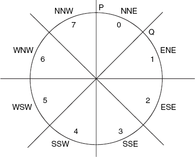
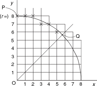
As in the previous sections, we begin with a simple case: we use the origin of the coordinate system as the center of the circle, and, dividing the circle into eight arcs of equal length, we restrict ourselves to one of these, the arc PQ. The points P(0, r) and Q
The equation of this circle is
Figure 4.6 shows the situation, including the grid of pixels, for the case r = 8. Beginning at the top at point P, with x = 0 and y = r, we will use a loop in which we increase x by 1 in each step; as in the previous section, we need some test to decide whether we can leave y unchanged. If not, we have to decrease y by 1.
Since, just after increasing x by 1, we have to choose between (x, y) and (x, y – 1), we could simply compute both
to see which lies closer to r2. Note that this can be done by using only integer arithmetic, so that in principle our problem is solved. To make our algorithm faster, we will avoid computing the squares x2 and y2, by introducing the three new, non-negative integer variables u, v and E denoting the differences between two successive squares and the 'error':
Initially, we have x = 0 and y = r, so that u = 1, v = 2r – 1 and E = 0. In each step in the loop, we increase x by 1, as previously discussed. Since, according to Equation (4.9), this will increase the value of x2 by u, we also have to increase E by u to satisfy Equation (4.11). We can also see from Equation (4.9) that increasing x by 1 implies that we have to increase u by 2. We now have to decide whether or not to decrease y by 1. If we do, Equation (4.10) indicates that the square y2 decreases by v, so that according to Equation (4.11) E also has to decrease by v. Since we want the absolute value of the error E to be as small as possible, the test we are looking for can be written
We will decrease y by 1 if and only if this test succeeds. It is interesting that we can write the condition (4.12) in a simpler form, by first replacing it with the equivalent test
| (E – v)2 < E2 |
which can be simplified to
| v(v – 2E) < 0 |
Since v is positive, we can simplify this further to
| v < 2E |
On the basis of the above discussion, we can now write the following method to draw the arc PQ (in which we write e instead of E):
void arc8(Graphics g, int r)
{  int x = 0, y = r, u = 1, v = 2 * r - 1, e = 0;
   while (x <= y)
   {  putPixel(g, x, y);
      x++; e += u; u += 2;
      if (v < 2 * e){y--; e -= v; v -= 2;}
   }
}
Equation (4.10) and Equation (4.11) show that in the case of decreasing y by 1, we have to decrease E by v and v by 2, as implemented in the if-statement. Note the symmetry between the three actions (related to y) in the if-statement and those (related to x) in the preceding program line.
The method arc8 is the basis for our final method, drawCircle, listed below. Besides drawing a full circle, it is also more general than arc8 in that it allows an arbitrary point C to be specified as the center of the circle. The comments in this method indicate directions of the compass. For example, NNE stands for north-north-east, which we use to refer to the arc between the north and the north-east directions (see Figure 4.5). As usual, we think of the y-axis pointing upward, so that y = r corresponds to north:
void drawCircle(Graphics g, int xC, int yC, int r)
{  int x = 0, y = r, u = 1, v = 2 * r - 1, e = 0;
   while (x < y)
   {  putPixel(g, xC + x, yC + y); // NNE
      putPixel(g, xC + y, yC - x); // ESE
      putPixel(g, xC - x, yC - y); // SSW
      putPixel(g, xC - y, yC + x); // WNW
      x++; e += u; u += 2;
      if (v < 2 * e){y--; e -= v; v -= 2;}
      if (x > y) break;
      putPixel(g, xC + y, yC + x); // ENE
      putPixel(g, xC + x, yC - y); // SSE
      putPixel(g, xC - y, yC - x); // WSW
      putPixel(g, xC - x, yC + y); // NNW
   }
}
This version has been programmed in such a way that putPixel will not visit the same pixel more than once. This is important if we want to use the XOR paint mode, writing
g.setXORMode(Color.white);
before the call to drawCircle. Setting the paint mode in this way implies that black pixels are made white and vice versa, so that we can remove a circle in the same way as we draw it. It is then essential that a single call to drawCircle does not put the same pixel twice on the screen, for then it would be erased the second time. To prevent pixels from being used twice, the eight calls to putPixel in the loop are divided into two groups of four: those in the first group draw the arcs 0, 2, 4 and 6 (see Figure 4.5), which include the starting points (0, r), (r, 0), (0, –r) and (–r, 0). The arcs 1, 3, 5 and 7 of the second group do not include these starting points because these calls to putPixel take place after x has been increased. As for the endpoint of each arc, we take care (a) that x is not greater than y for any call to putPixel, and (b) that the situation x = y is covered by at most one of these two groups of putPixel calls. This situation will occur, for example, if r = 6; in this case the following eight points (relative to the center of the circle) are selected in this order, as far as the north-east quadrant of the circle (NNE and ENE) is concerned: (0, 6), (6, 1), (1, 6), (6, 2), (2, 6), (5, 3), (3, 5), (4, 4). In this situation the test after while terminates the loop. In contrast, the situation x = y will not occur if r = 8, since in this case the eleven points (0, 8), (8, 1), (1, 8), (8, 2), (2, 8), (7, 3), (3, 7), (7, 4), (4, 7), (6, 5), (5, 6) are chosen, in that order. The loop now terminates because the break-statement in the middle of it is executed.
In this section we will discuss how to draw line segments only as far as they lie within a given rectangle. For example, given a point P inside and a point Q outside a rectangle. It is then our task to draw only the line segment PI, where I is the point of intersection of PQ and the rectangle, as shown in Figure 4.7. The rectangle is given by the four numbers xmin, xmax, ymin and ymax. These four values and the coordinates of P and Q are floating-point logical coordinates, as usual.
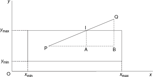
Since PQ intersects the upper edge of the rectangle in I, we have
| yI = ymax |
As the triangles PAI and PBQ are similar, we can write
After replacing yI with ymax and multiplying both sides of this equation by ymax – yP, we easily obtain
so that we can draw the desired line segment PI.
This easy way of computing the coordinates of point I is based on several facts that apply to Figure 4.7, but that must not be relied on in a general algorithm. For example, if Q lies farther to the right, it may not be immediately clear whether the point of intersection lies on the upper edge y = ymax or on the right edge x = xmax. In general, there are many more cases to consider. The logical decisions needed to find out which actions to take make line clipping an interesting topic from an algorithmic point of view. The Cohen–Sutherland algorithm solves this problem in an elegant and efficient way. We will express this algorithm in Java.
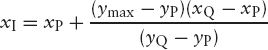
The four lines x = xmin, x = xmax, y = ymin, y = ymax divide the xy-plane into nine regions. With any point P(x, y) we associate a four-bit code
| b3 b2 b1 b0 |
identifying that region, as Figure 4.8 shows.
For any point (x, y), the above four-bit code is defined as follows:
| b3 = 1 if and only if x < xmin |
| b2 = 1 if and only if x > xmax |
| b1 = 1 if and only if y < ymin |
| b0 = 1 if and only if y > ymax |
Based on this code, the Cohen–Sutherland algorithm replaces the endpoints P and Q of a line segment, if they lie outside the rectangle, with points of intersection of PQ and the rectangle, that is, if there are such points of intersection. This is done in a few steps. For example, in Figure 4.8, the following steps are taken:
Since P lies to the left of the left rectangle edge, it is replaced with P′ (on x = xmin), so that only P′Q remains to be dealt with.
Since P′ lies below the lower rectangle edge, it is replaced with P″ (on y = ymin), so that P″Q remains to be dealt with.
Since Q lies to the right of the right rectangle edge, it is replaced with Q′ (on x = xmax), so that P″Q′ remains to be dealt with.
Line segment P″Q′ is drawn.
Steps 1, 2 and 3 are done in a loop, which can terminate in two ways:
If the four-bit codes of P (or P′ or P″, which we again refer to as P in the program) and of Q are equal to zero; the (new) line segment PQ is then drawn.
If the two four-bit codes contain a 1-bit in the same position; this implies that P and Q are on the same side of a rectangle edge, so that nothing has to be drawn.
The method clipLine in the following program shows this in greater detail:
// ClipLine.java: Cohen-Sutherland line clipping.
import java.awt.*;
import java.awt.event.*;
import java.util.*;

public class ClipLine extends Frame
{  public static void main(String[] args){new ClipLine();}

   ClipLine()
   {  super("Click on two opposite corners of a rectangle");
      addWindowListener(new WindowAdapter()
         {public void windowClosing(WindowEvent e){System.exit(0);}});
      setSize (500, 300);
      add("Center", new CvClipLine());

      setCursor(Cursor.getPredefinedCursor(Cursor.CROSSHAIR_CURSOR));
      show();
   }
}

class CvClipLine extends Canvas
{  float xmin, xmax, ymin, ymax,
      rWidth = 10.0F, rHeight = 7.5F, pixelSize;
   int maxX, maxY, centerX, centerY, np=0;

   CvClipLine()
   {  addMouseListener(new MouseAdapter()
      {  public void mousePressed(MouseEvent evt)
{ float x = fx(evt.getX()), y = fy(evt.getY());
if (np == 2) np = 0;
if (np == 0){xmin = x; ymin = y;}
else
{ xmax = x; ymax = y;
if (xmax < xmin)
{ float t = xmax; xmax = xmin; xmin = t;
}
if (ymax < ymin)
{ float t = ymax; ymax = ymin; ymin = t;
}
}
np++;
repaint();
}
});
}
void initgr()
{ Dimension d = getSize();
maxX = d.width - 1; maxY = d.height - 1;
pixelSize = Math.max(rWidth/maxX, rHeight/maxY);
centerX = maxX/2; centerY = maxY/2;
}
int iX(float x){return Math.round(centerX + x/pixelSize);}
int iY(float y){return Math.round(centerY - y/pixelSize);}
float fx(int x){return (x - centerX) * pixelSize;}
float fy(int y){return (centerY - y) * pixelSize;}
void drawLine(Graphics g, float xP, float yP,
float xQ, float yQ)
{ g.drawLine(iX(xP), iY(yP), iX(xQ), iY(yQ));
}
int clipCode(float x, float y)
{ return
(x < xmin ? 8 : 0) | (x > xmax ? 4 : 0) |
(y < ymin ? 2 : 0) | (y > ymax ? 1 : 0);
}
void clipLine(Graphics g,
float xP, float yP, float xQ, float yQ,float xmin, float ymin, float xmax, float ymax)
{ int cP = clipCode(xP, yP), cQ = clipCode(xQ, yQ);
float dx, dy;
while ((cP | cQ) != 0)
{ if ((cP & cQ) != 0) return;
dx = xQ - xP; dy = yQ - yP;
if (cP != 0)
{ if ((cP & 8) == 8){yP += (xmin-xP) * dy / dx; xP = xmin;}
else
if ((cP & 4) == 4){yP += (xmax-xP) * dy / dx; xP = xmax;}
else
if ((cP & 2) == 2){xP += (ymin-yP) * dx / dy; yP = ymin;}
else
if ((cP & 1) == 1){xP += (ymax-yP) * dx / dy; yP = ymax;}
cP = clipCode(xP, yP);
}
else
if (cQ != 0)
{ if ((cQ & 8) == 8){yQ += (xmin-xQ) * dy / dx; xQ = xmin;}
else
if ((cQ & 4) == 4){yQ += (xmax-xQ) * dy / dx; xQ = xmax;}
else
if ((cQ & 2) == 2){xQ += (ymin-yQ) * dx / dy; yQ = ymin;}
else
if ((cQ & 1) == 1){xQ += (ymax-yQ) * dx / dy; yQ = ymax;}
cQ = clipCode(xQ, yQ);
}
}
drawLine(g, xP, yP, xQ, yQ);
}
public void paint(Graphics g)
{ initgr();
if (np == 1)
{ // Draw horizontal and vertical lines through
// first defined point:
drawLine(g, fx (0) , ymin, fx(maxX), ymin);
drawLine(g, xmin, fy (0) , xmin, fy(maxY));
} else
if (np == 2)
{ // Draw rectangle:
drawLine(g, xmin, ymin, xmax, ymin);
drawLine(g, xmax, ymin, xmax, ymax);
drawLine(g, xmax, ymax, xmin, ymax);drawLine(g, xmin, ymax, xmin, ymin);
// Draw 20 concentric regular pentagons, as
// far as they lie within the rectangle:
float rMax = Math.min(rWidth, rHeight)/2,
deltaR = rMax/20, dPhi = (float)(0.4 * Math.PI);
for (int j=1; j<'=20; j++)
{ float r = j * deltaR;
// Draw a pentagon:
float xA, yA, xB = r, yB = 0;
for (int i=1; i<=5; i++)
{ float phi = i * dPhi;
xA = xB; yA = yB;
xB = (float)(r * Math.cos(phi));
yB = (float)(r * Math.sin(phi));
clipLine(g, xA, yA, xB, yB, xmin, ymin, xmax, ymax);
}
}
}
}
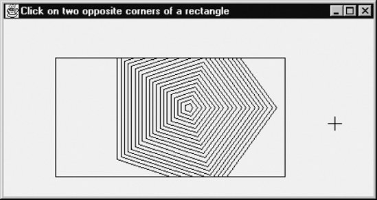
}The program draws 20 concentric (regular) pentagons, as far as these lie within a rectangle, which the user can define by clicking on any two opposite corners. When he or she clicks for the third time, the situation is the same as at the beginning: the screen is cleared and a new rectangle can be defined, in which again parts of 20 pentagons appear, and so on. As usual, if the user changes the window dimensions, the size of the result is changed accordingly. Figure 4.9 shows the situation just after the pentagons are drawn.
If we look at the while-loop in the method clipLine, it seems that this code is somewhat inefficient because of the divisions dy/dx and dx/dy inside that loop while dx and dy are not changed in it. However, we should bear in mind that dx or dy may be zero. The if-statements in the loop guarantee that no division by dx or dy will be performed if that variable is zero. Besides, this loop is different from most other program loops in that the inner part is usually executed only once or not at all, and rarely more than once.
In contrast to line clipping, discussed in the previous section, we will now deal with polygon clipping, which is different in that it converts one polygon into another within a given rectangle, as Figures 4.10 and 4.11 illustrate.
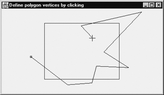
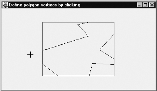
The program that we will discuss draws a fixed rectangle and enables the user to specify the vertices of a polygon by clicking, in the same way as discussed in Section 1.5. As long as the first vertex, in Figure 4.10 on the left, is not selected for the second time, successive vertices are connected by polygon edges. As soon as the first vertex is selected again, the polygon is clipped, as Figure 4.11 shows. Some vertices of the original polygon do not belong to the clipped one. On the other hand, the latter polygon has some new vertices, which are all points of intersection of the edges of the original polygon and those of the rectangle. In general, the number of vertices of the clipped polygon can be greater than, equal to or less than that of the original one. In Figure 4.11 there are five new polygon edges, which are part of the rectangle edges.
The program that produced Figure 4.11 is based on the Sutherland–Hodgman algorithm, which first clips all polygon edges against one rectangle edge, or rather, the infinite line through such an edge. This results in a new polygon, which is then clipped against the next rectangle edge, and so on. Figure 4.12 shows a rectangle and a polygon, ABCDEF. Starting at vertex A, we find that AB intersects the line x = xmax in point I, which will be a new vertex of the clipped polygon. The same applies to point J, the point of intersection of DE with the same vertical rectangle edge.
Let us refer to the original polygon as the input polygon and the new one as the output polygon. We represent each polygon by a sequence of successive vertices. Let us start with the right rectangle edge and treat it as an infinite clipping line, which can be expressed as x = xmax, and see how to clip the polygon against this line. In general, when working on one clipping line, we ignore all other rectangle edges. Initially, the output polygon is empty. When following all successive polygon edges such as AB, we focus on the endpoint, B, and decide as follows which points will belong to the output polygon:
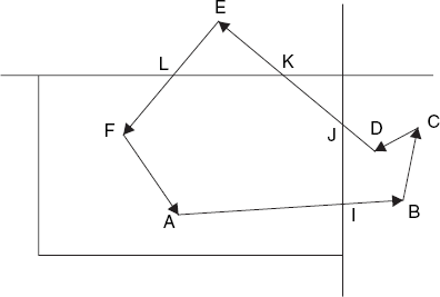
If A and B lie on different sides of the clipping line, the point of intersection, I, is added to the output polygon. Regardless of this being the case, B is added to the output polygon if and only if it lies on the same side of the clipping line as the rectangle.
Starting with the directed edge AB in Figure 4.12, point I is the first to be added to the output polygon. Vertex B is not added because it is not on the same side of the clipping line as the rectangle, and the same applies to the endpoints of the following directed edges, BC and CD. When dealing with edge DE, we first add J and then E to the output polygon since they are both on the same side of the clipping line as the rectangle. The endpoints of the next two edges, EF and FA, lie on the same side of the clipping line as the rectangle and are therefore added to the output polygon. In this way we obtain the vertices I, J, E, F and A, in that order. We then use this output polygon as the input polygon to clip against the top rectangle edge. Using the same method as described above on the right edge, we obtain the vertices I, J, K, L, F and A, which forms the output polygon IJKLFA. Although in this example IJKLFA is the desired clipped polygon, it will in general be necessary to use the output polygon as input for working with another rectangle edge. The program below shows an implementation in Java:
// ClipPoly.java: Clipping a polygon.
// Uses: Point2D (Section 1.5).
import java.awt.*;
import java.awt.event.*;
import java.util.*;
public class ClipPoly extends Frame
{  public static void main(String[] args){new ClipPoly();}

   ClipPoly()
   {  super("Define polygon vertices by clicking");
      addWindowListener(new WindowAdapter()
         {public void windowClosing(WindowEvent e)
                 {System.exit(0);}});
      setSize (500, 300);
      add("Center", new CvClipPoly());

      setCursor(Cursor.getPredefinedCursor
                     (Cursor.CROSSHAIR_CURSOR));
      show();
   }
}

class CvClipPoly extends Canvas
{  Poly poly = null;
   float rWidth = 10.0F, rHeight = 7.5F, pixelSize;
   int x0, y0, centerX, centerY;
   boolean ready = true;

   CvClipPoly()
   {  addMouseListener(new MouseAdapter()
      {  public void mousePressed(MouseEvent evt)
         {  int x = evt.getX(), y = evt.getY();
            if (ready)
            {  poly = new Poly();
               x0 = x; y0 = y;
               ready = false;
            }
            if (poly.size() > 0 &&
               Math.abs(x - x0) < 3 && Math.abs(y - y0) < 3)
               ready = true;
            else
               poly.addVertex(new Point2D(fx(x), fy(y)));
            repaint();
         }
      });
   }
void initgr()
{ Dimension d = getSize();
int maxX = d.width - 1, maxY = d.height - 1;
pixelSize = Math.max(rWidth/maxX, rHeight/maxY);
centerX = maxX/2; centerY = maxY/2;
}
int iX(float x){return Math.round(centerX + x/pixelSize);}
int iY(float y){return Math.round(centerY - y/pixelSize);}
float fx(int x){return (x - centerX) * pixelSize;}
float fy(int y){return (centerY - y) * pixelSize;}
void drawLine(Graphics g, float xP, float yP, float xQ,
float yQ)
{ g.drawLine(iX(xP), iY(yP), iX(xQ), iY(yQ));
}
void drawPoly(Graphics g, Poly poly)
{ int n = poly.size();
if (n == 0) return;
Point2D a = poly.vertexAt(n − 1);
for (int i=0; i<n; i++)
{ Point2D b = poly.vertexAt(i);
drawLine(g, a.x, a.y, b.x, b.y);
a = b;
}
}
public void paint(Graphics g)
{ initgr();
float xmin = -rWidth/3, xmax = rWidth/3,
ymin = -rHeight/3, ymax = rHeight/3;
// Draw clipping rectangle:
g.setColor(Color.blue);
drawLine(g, xmin, ymin, xmax, ymin);
drawLine(g, xmax, ymin, xmax, ymax);
drawLine(g, xmax, ymax, xmin, ymax);
drawLine(g, xmin, ymax, xmin, ymin);
g.setColor(Color.black);
if (poly == null) return;
int n = poly.size();
if (n == 0) return;
Point2D a = poly.vertexAt (0);if (!ready)
{ // Show tiny rectangle around first vertex:
g.drawRect(iX(a.x)−2, iY(a.y)−2, 4, 4);
// Draw incomplete polygon:
for (int i=1; i<n; i++)
{ Point2D b = poly.vertexAt(i);
drawLine(g, a.x, a.y, b.x, b.y);
a = b;
}
} else
{ poly.clip(xmin, ymin, xmax, ymax);
drawPoly(g, poly);
}
}
}
class Poly
{ Vector v = new Vector();
void addVertex(Point2D p){v.addElement(p);}
int size(){return v.size();}
Point2D vertexAt(int i)
{ return (Point2D)v.elementAt(i);
}
void clip(float xmin, float ymin, float xmax, float ymax)
{ // Sutherland-Hodgman polygon clipping:
Poly poly1 = new Poly();
int n;
Point2D a, b;
boolean aIns, bIns; // whether A or B is on the same
// side as the rectangle
// Clip against x == xmax:
if ((n = size()) == 0) return;
b = vertexAt(n-1);
for (int i=0; i<n; i++)
{ a = b; b = vertexAt(i);
aIns = a.x <= xmax; bIns = b.x <= xmax;
if (aIns != bIns)
poly1.addVertex(new Point2D(xmax, a.y +
(b.y - a.y) * (xmax - a.x)/(b.x - a.x)));
if (bIns) poly1.addVertex(b);
}v = poly1.v; poly1 = new Poly();
// Clip against x == xmin:
if ((n = size()) == 0) return;
b = vertexAt(n-1);
for (int i=0; i<n; i++)
{ a = b; b = vertexAt(i);
aIns = a.x >= xmin; bIns = b.x >= xmin;
if (aIns != bIns)
poly1.addVertex(new Point2D(xmin, a.y +
(b.y - a.y) * (xmin − a.x)/(b.x - a.x)));
if (bIns) poly1.addVertex(b);
}
v = poly1.v; poly1 = new Poly();
// Clip against y == ymax:
if ((n = size()) == 0) return;
b = vertexAt(n-1);
for (int i=0; i<n; i++)
{ a = b; b = vertexAt(i);
aIns = a.y <= ymax; bIns = b.y <= ymax;
if (aIns != bIns)
poly1.addVertex(new Point2D(a.x +
(b.x - a.x) * (ymax - a.y)/(b.y - a.y), ymax));
if (bIns) poly1.addVertex(b);
}
v = poly1.v; poly1 = new Poly();
// Clip against y == ymin:
if ((n = size()) == 0) return;
b = vertexAt(n-1);
for (int i=0; i<n; i++)
{ a = b; b = vertexAt(i);
aIns = a.y >= ymin;
bIns = b.y >= ymin;
if (aIns != bIns)
poly1.addVertex(new Point2D(a.x +
(b.x - a.x) * (ymin − a.y)/(b.y - a.y), ymin));
if (bIns) poly1.addVertex(b);
}
v = poly1.v; poly1 = new Poly();
}
}The Sutherland–Hodgman algorithm can be adapted for clipping regions other than rectangles and for three-dimensional applications.
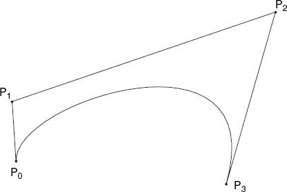
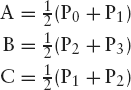
There are many algorithms for constructing curves. A particularly elegant and practical one is based on specifying four points that completely determine a curve segment: two endpoints and two control points. Curves constructed in this way are referred to as (cubic) Bézier curves. In Figure 4.13, we have the endpoints P0 and P3, the control points P1 and P2, and the curve constructed on the basis of these four points.
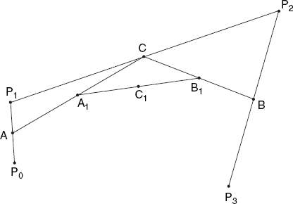
Writing a method to draw this curve is surprisingly easy, provided we use recursion. As Figure 4.14 shows, we compute six midpoints, namely:
A, the midpoint of P0P1
B, the midpoint of P2P3
C, the midpoint of P1P2
A1, the midpoint of AC
B1, the midpoint of BC
C1, the midpoint of A1B1
After this, we can divide the original task of drawing the Bézier curve P0P3 (with control points P1 and P2 into two simpler tasks:
drawing the Bézier curve P0C1, with control points A and A1
drawing the Bézier curve C1P3, with control points B1 and B
All this needs to be done only if the original points P0 and P3 are further apart than some small distance, say, ɛ. Otherwise, we simply draw the straight line P0P3. Since we are using pixels on a raster, we can also base the test just mentioned on device coordinates: we will simply draw a straight line from P0 to P3 if and only if the corresponding pixels are neighbors or identical, writing
if (Math.abs(x0 - x3) <= 1 && Math.abs(y0 - y3) <= 1)
      g.drawLine(x0, y0, x3, y3);
else ...
The recursive method bezier in the following program shows an implementation of this algorithm. The program expects the user to specify the four points P0, P1, P2 and P3, in that order, by clicking the mouse. After the fourth point, P3, has been specified, the curve is drawn. Any new mouse clicking is interpreted as the first point, P0, of a new curve; the previous curve simply disappears and another curve can be constructed in the same way as the first one, and so on.
// Bezier.java: Bezier curve segments.
// Uses: Point2D (Section 1.5).

import java.awt.*;
import java.awt.event.*;
import java.util.*;

public class Bezier extends Frame
{  public static void main(String[] args){new Bezier();}
Bezier()
{ super("Define endpoints and control points of curve segment");
addWindowListener(new WindowAdapter()
{public void windowClosing(WindowEvent e){System.exit(0);}});
setSize (500, 300);
add("Center", new CvBezier());
setCursor(Cursor.getPredefinedCursor(Cursor.CROSSHAIR_CURSOR));
show();
}
}
class CvBezier extends Canvas
{ Point2D[] p = new Point2D[4];
int np = 0, centerX, centerY;
float rWidth = 10.0F, rHeight = 7.5F, eps = rWidth/100F, pixelSize;
CvBezier()
{ addMouseListener(new MouseAdapter()
{ public void mousePressed(MouseEvent evt)
{ float x = fx(evt.getX()), y = fy(evt.getY());
if (np == 4) np = 0;
p[np++] = new Point2D(x, y);
repaint();
}
});
}
void initgr()
{ Dimension d = getSize();
int maxX = d.width - 1, maxY = d.height - 1;
pixelSize = Math.max(rWidth/maxX, rHeight/maxY);
centerX = maxX/2; centerY = maxY/2;
}
int iX(float x){return Math.round(centerX + x/pixelSize);}
int iY(float y){return Math.round(centerY - y/pixelSize);}
float fx(int x){return (x - centerX) * pixelSize;}
float fy(int y){return (centerY - y) * pixelSize;}
Point2D middle(Point2D a, Point2D b)
{ return new Point2D((a.x + b.x)/2, (a.y + b.y)/2);
}void bezier(Graphics g, Point2D p0, Point2D p1,
Point2D p2, Point2D p3)
{ int x0 = iX(p0.x), y0 = iY(p0.y),
x3 = iX(p3.x), y3 = iY(p3.y);
if (Math.abs(x0 - x3) <= 1 && Math.abs(y0 - y3) <= 1)
g.drawLine(x0, y0, x3, y3);
else
{ Point2D a = middle(p0, p1), b = middle(p3, p2),
c = middle(p1, p2), a1 = middle(a, c),
b1 = middle(b, c), c1 = middle(a1, b1);
bezier(g, p0, a, a1, c1);
bezier(g, c1, b1, b, p3);
}
}
public void paint(Graphics g)
{ initgr();
int left = iX(-rWidth/2), right = iX(rWidth/2),
bottom = iY(-rHeight/2), top = iY(rHeight/2);
g.drawRect(left, top, right - left, bottom - top);
for (int i=0; i<np; i++)
{ // Show tiny rectangle around point:
g.drawRect(iX(p[i].x)−2, iY(p[i].y)−2, 4, 4);
if (i > 0)
// Draw line p[i-1]p[i]:
g.drawLine(iX(p[i-1].x), iY(p[i-1].y),
iX(p[i].x), iY(p[i].y));
}
if (np == 4) bezier(g, p[0], p[1], p[2], p[3]);
}
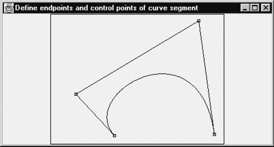
}Since this program uses the isotropic mapping mode with logical coordinate ranges 0–10.0 for x and 0–7.5 for y, we should only use a rectangle whose height is 75% of its width. As in Sections 1.4 and 1.5, we place this rectangle at the center of the screen and make it as large as possible. It is shown in Figure 4.15; if the four points for the curve are chosen within this rectangle, they will be visible regardless of how the size of the window is changed by the user. The same applies to the curve, which is automatically scaled, in the same way as we did in Sections 1.4 and 1.5.
This way of constructing a Bézier curve may look like magic. To understand what is going on, we must be familiar with the notion of parametric representation, which, in 2D, we can write as
where t is a parameter, which we may think of as time. Variable t ranges from 0 to 1: as if we move from P0 to P3 with constant velocity, starting at t = 0 and finishing at t = 1. At time t = 0.5 we are half-way. With cubic Bézier curves, both f(t) and g(t) are third degree polynomials in t.
Before we proceed, let us pay some attention to expressions such as
to compute the midpoint A of line segment P0P1. The points in such expressions actually denote vectors, which enables us to form their sum and to multiply them by a scalar. Without this shorthand notation, we would have to write
which would be rather awkward. Let us write each Pi as the column vector
(where we have taken the liberty of mixing mathematical and programming notations). In the same way, we combine the above functions f(t) and g(t),
writing
Then the cubic Bézier curve is defined as follows:
Substituting 0 and 1 for t, we find B(0) = P0 and B(1) = P3. Before discussing the relation between this definition and the recursive midpoint construction, let us see this definition in action. It enables us to replace the recursive method bezier with the following non-recursive one:
void bezier1(Graphics g, Point2D[] p)
{  int n = 200;
   float dt = 1.0F/n, x = p[0].x, y = p[0].y, x0, y0;
   for (int i=1; i<=n; i++)
   {  float t = i * dt, u = 1 - t,
         tuTriple = 3 * t * u,
         c0 = u * u * u,
         c1 = tuTriple * u,
         c2 = tuTriple * t,
         c3 = t * t * t;
       x0 = x; y0 = y;
       x = c0*p[0].x + c1*p[1].x + c2*p[2].x + c3*p[3].x;
       y = c0*p[0].y + c1*p[1].y + c2*p[2].y + c3*p[3].y;
       g.drawLine(iX(x0), iY(y0), iX(x), iY(y));
   }
}
This method produces the same curve as that produced by bezier, provided we also replace the call to bezier with this one:
bezier1(g, P);
We will discuss a more efficient non-recursive method, bezier2, equivalent to bezier1, at the end of this section.
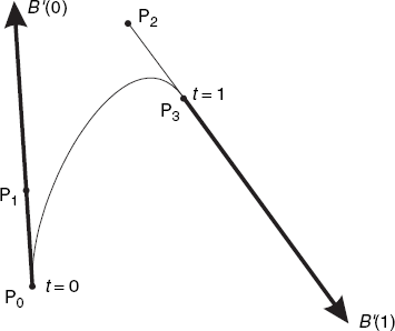
Since B(t) denotes the position at time t, the derivative B′(t) of this function (which is also a column vector depending on t) can be regarded as the velocity. After some algebraic manipulation and differentiating, we find
which gives
| B′(0) = 3(P1 – P0) |
| B′(1) = 3(P3 – P2) |
These two results are velocity vectors at the starting point P0 and the endpoint P3. They show that the direction we move at on these points is along the vectors P0 P1 and P2P3, as Figure 4.16 illustrates.
We have been discussing two entirely different ways to construct a curve between the points P0 and P3, and, without an experiment, it is not clear that these curves are identical. For the time being, we will distinguish between the two curves and refer to them as
the midpoint curve, constructed by a recursive process of computing midpoints, and implemented in the method bezier;
the analytical curve, given by Equation (4.13) and implemented in the method bezier1.
Although both methods are based on the four points P0, P1, P2 and P3, the ways we compute hundreds of curve points (to connect them by tiny straight lines) are very different. It would be unsatisfactory if it remained a mystery why these curves are identical. Let us therefore briefly discuss a way to prove this fact.
Using the function B(t) of Equation (4.13), we find
Since point C1 in Figure 4.14 was used to divide the whole midpoint curve into two smaller curves, we might suspect that C1 and B(0.5) are two different expressions for the same point. We verify this by expressing C1 in terms of the four given points, using Figure 4.14. Because C1 is the midpoint of A1B1 and both A1 and B1 are also midpoints, and so on, we find
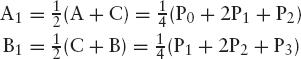
which is indeed the expression that we found for B(0.5). This proves that point C1, which obviously belongs to the midpoint curve, also lies on the analytical curve. Besides P0 and P3, there is now only one point, C1, which we have proved lies on both curves, so it seems we are still far away from the proof that these curves are identical. However, we can now apply the same argument recursively, which would enable us to find as many points that lie on both curves as we like. Restricting ourselves to the first half of each curve, we focus on the points P0, A, A1 and C1, which we can again use to construct both midpoint and analytical curves. For the latter we use the following equation, which is similar to Equation (4.13):
It is then obvious that b(0)= P0, b(1) = C1 and b(0.5) is identical with a midpoint (between P0 and C1) used in the recursive process, in the same way as B(0.5) is identical with the midpoint C1. There is one remaining difficulty: is the analytical curve given by Equation (4.18) really the same as the first part of that given by Equation (4.13)? We will show that this is indeed the case. Using u = 2t (since u = 1 and t = 0.5 at point C1) we have
| b(u) = B(t) |
To verify this, note that, according to Equation (4.18), we have
Using Equations (4.15), (4.16) and Equation (4.17), we can write the last expression as

Rearranging this formula, we find that it is equal to the expression for B(t) in Equation (4.13), which is what we had to prove.
Suppose that we want to combine two Bézier curve segments, one based on the four points P0, P1, P2, P3 and the other on Q0, Q1, Q2 and Q3, in such a way that the endpoint P3 of the first segment coincides with the starting point Q0 of the second. Then the combined curve will be smoothest if the final velocity B′(1) (see Figure 4.16) of the first segment is equal to the initial velocity B′(0) of the second. This will be the case if the point P3 (= Q0) lies exactly at the middle of the line segment P2Q1. The high degree of smoothness obtained in this way is referred to as second-order continuity. It implies not only that the two segments have the same tangent at their common point P3 = Q0, but also that the curvature is continuous at this point. By contrast, we have first-order continuity if P3 lies on the line segment P2Q1 but not at the middle of it. In this case, although the curve looks reasonably smooth because both segments have the same tangent in the common point P3 = Q0, there is a discontinuity in the curvature at this point.
It will be clear that we can write Equation (4.13) as follows:

Since the row vector in this matrix product is equal to
we can also write it as the product of a simpler row vector, [t3 t2 t 1], and a 4 × 4 matrix, obtaining the following result for the Bézier curve:
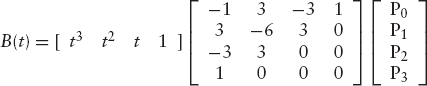
As we know, any matrix product ABC of three matrices is equal to both (AB)C and A(BC). If we do the first matrix multiplication first, as in (AB)C, Equation (4.20) reduces to Equation (4.19). On the other hand, if we do the second first, as in A(BC), we obtain the following result:
| B(t) = (–P0 + 3P1 – 3P2 + P3)t3 + 3(P0 – 2P1 + P3)t2 – 3(P1 – P0)t + P0 |
This is interesting because it provides us with a very efficient way of drawing a Bézier curve segment, as the following improved method shows:
void bezier2(Graphics g, Point2D[] p)
{  int n = 200;
   float dt = 1.0F/n,
   cx3 = -p[0].x + 3 * (p[1].x - p[2].x) + p[3].x,
   cy3 = -p[0].y + 3 * (p[1].y - p[2].y) + p[3].y,
   cx2 = 3 * (p[0].x - 2 * p[1].x + p[2].x),
   cy2 = 3 * (p[0].y - 2 * p[1].y + p[2].y),
   cx1 = 3 * (p[1].x - p[0].x),
   cy1 = 3 * (p[1].y - p[0].y),
   cx0 = p[0].x,
   cy0 = p[0].y,
   x = p[0].x, y = p[0].y, x0, y0;
   for (int i=1; i<=n; i++)
   {  float t = i * dt;
      x0 = x; y0 = y;
      x = ((cx3 * t + cx2) * t + cx1) * t + cx0;
      y = ((cy3 * t + cy2) * t + cy1) * t + cy0;
      g.drawLine(iX(x0), iY(y0), iX(x), iY(y));
   }
}
The above computation of x and y is an application of Horner's rule, according to which we can efficiently compute polynomials by using the right-hand rather than the left-hand side of the following equation:
| a3t3 + a2t2 + a1t + a0 = ((a3t + a2)t + a1)t + a0 |
Although bezier2 does not look simpler than bezier1, it is much more efficient because of the reduced number of arithmetic operations in the for-loop. With a large number of steps, such as n = 200 in these versions of bezier1 and bezier2, it is the number of operations inside the loop that counts, not the preparatory actions that precede the loop.
Although the curves discussed here are two-dimensional, three-dimensional curves can be generated in the same way. We simply add a z-component to B(t) and to the control points, and compute this in the same way as the x- and y-components are computed. The possibility of generating curves that do not lie in a plane is related to the degree of the polynomials we have been discussing. If the four given points do not lie in the same plane, the generated cubic curve segment does not either. By contrast, quadratic curves are determined by only three points, which uniquely define a plane (unless they are collinear); the quadratic curve through those three points lies in that plane. In other words, polynomial curves can be non-planar only if they are at least of degree 3.
Besides the techniques discussed in the previous section, there are other ways of generating curves x = f(t), y = g(t), where f and g are polynomials in t of degree 3. A popular one, known as B-splines, has the characteristic that the generated curve will normally not pass through the given points. We will refer to all these points as control points. A single segment of such a curve, based on four control points A, B, C and D, looks rather disappointing in that it seems to be related only to B and C. This is shown in Figure 4.17, in which, from left to right, the points A, B, C and D are again marked with tiny squares.
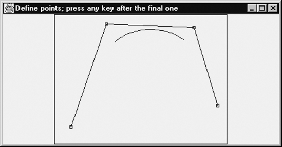
However, a strong point in favor of B-splines is that this technique makes it easy to draw a very smooth curve consisting of many curve segments. To avoid confusion, note that each curve segment consists of many straight-line segments. For example, Figure 4.17 shows one curve segment which consists of 50 line segments. Since four control points are required for a single curve segment, we have
| number of control points = number of curve segments + 3 |
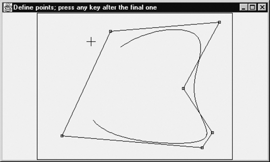
in this case. This equation also applies if there are several curve segments. At first sight, Figure 4.18 seems to violate this rule, since there are five curve segments, and it looks as if there are only six control points. However, two of these were used twice. This curve was constructed by clicking first on the lower-left vertex (= point 0), followed by clicking on the upper-left one (= point 1), then the upper-right one (= point 2), and so on, following the polygon clockwise. Altogether, the eight control points 0, 1, 2, 3, 4, 5, 0, 1 were selected, in that order. If after this, a key on the keyboard is pressed, only the curve is redrawn, not the control points and the lines that connect them.
If we had clicked on yet another control point (point 2, at the top, right), we would have had a closed curve. In general, to produce a closed curve, there must be three overlapping vertices, that is, two overlapping polygon edges. As you can see in Figure 4.18, the curve is very smooth indeed: we have second-order continuity, as discussed in the previous section. Recall that this implies that even the curvature is continuous in the points where two adjacent curve segments meet. As the part of the curve near the lower-right corner shows, we can make the distance between a curve and the given points very small by supplying several points close together.
The mathematics of B-splines can be expressed by the following matrix equation, similar to Equation (4.20):
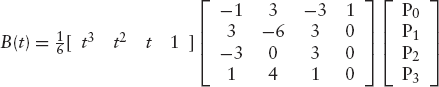
If we have n control points P0, P1, . . ., Pn−1 (n ≥ 4) then, strictly speaking, Equation (4.21) applies only to the first curve segment. For the second, we have to replace the points P0, P1, P2 and P3 in the column vector with P1, P2, P3 and P4, and so on. As with Bézier curves, the variable t ranges from 0 to 1 for each curve segment. Multiplying the above 4 × 4 matrix by the column vector that follows it, we obtain
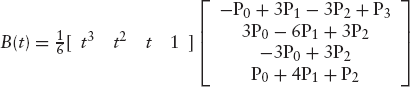
or

The following program is based on this equation. The user can click any number of points, which are used as the points P0, P1, . . ., Pn−1. The first curve segment appears immediately after the fourth control point, P3, has been defined, and each additional control point causes a new curve segment to appear. To show only the curve, the user can press any key, which also terminates the input process. After this, we can generate another curve by clicking again. The old curve then disappears. Figures 4.17 and 4.18 have been produced by this program:
// Bspline.java: B-spline curve fitting.
// Uses: Point2D (Section 1.5).

import java.awt.*;
import java.awt.event.*;
import java.util.*;

public class Bspline extends Frame
{  public static void main(String[] args){new Bspline();}

   Bspline()
   {  super("Define points; press any key after the final one");
      addWindowListener(new WindowAdapter()
         {public void windowClosing(WindowEvent e){System.exit(0);}});
      setSize (500, 300);
      add("Center", new CvBspline());

      setCursor(Cursor.getPredefinedCursor(Cursor.CROSSHAIR_CURSOR));
      show();
   }
}

class CvBspline extends Canvas
{ Vector V = new Vector();
int np = 0, centerX, centerY;
float rWidth = 10.0F, rHeight = 7.5F, eps = rWidth/100F, pixelSize;
boolean ready = false;
CvBspline()
{ addMouseListener(new MouseAdapter()
{ public void mousePressed(MouseEvent evt)
{ float x = fx(evt.getX()), y = fy(evt.getY());
if (ready)
{ V.removeAllElements();
np = 0;
ready = false;
}
V.addElement(new Point2D(x, y));
np++;
repaint();
}
});
addKeyListener(new KeyAdapter()
{ public void keyTyped(KeyEvent evt)
{ evt.getKeyChar();
if (np >= 4) ready = true;
repaint();
}
});
}
void initgr()
{ Dimension d = getSize();
int maxX = d.width - 1, maxY = d.height - 1;
pixelSize = Math.max(rWidth/maxX, rHeight/maxY);
centerX = maxX/2; centerY = maxY/2;
}
int iX(float x){return Math.round(centerX + x/pixelSize);}
int iY(float y){return Math.round(centerY - y/pixelSize);}
float fx(int x){return (x - centerX) * pixelSize;}
float fy(int y){return (centerY - y) * pixelSize;}
void bspline(Graphics g, Point2D[] p)
{ int m = 50, n = p.length;
float xA, yA, xB, yB, xC, yC, xD, yD,a0, a1, a2, a3, b0, b1, b2, b3, x=0, y=0, x0, y0;
boolean first = true;
for (int i=1; i<n-2; i++)
{ xA=p[i-1].x; xB=p[i].x; xC=p[i+1].x; xD=p[i+2].x;
yA=p[i-1].y; yB=p[i].y; yC=p[i+1].y; yD=p[i+2].y;
a3=(-xA+3*(xB-xC)+xD)/6; b3=(-yA+3*(yB-yC)+yD)/6;
a2=(xA−2*xB+xC)/2; b2=(yA−2*yB+yC)/2;
a1=(xC-xA)/2; b1=(yC-yA)/2;
a0=(xA+4*xB+xC)/6; b0=(yA+4*yB+yC)/6;
for (int j=0; j<=m; j++)
{ x0 = x;
y0 = y;
float t = (float)j/(float)m;
x = ((a3*t+a2)*t+a1)*t+a0;
y = ((b3*t+b2)*t+b1)*t+b0;
if (first) first = false;
else
g.drawLine(iX(x0), iY(y0), iX(x), iY(y));
}
}
}
public void paint(Graphics g)
{ initgr();
int left = iX(-rWidth/2), right = iX(rWidth/2),
bottom = iY(-rHeight/2), top = iY(rHeight/2);
g.drawRect(left, top, right - left, bottom - top);
Point2D[] p = new Point2D[np];
V.copyInto(p);
if (!ready)
{ for (int i=0; i<np; i++)
{ // Show tiny rectangle around point:
g.drawRect(iX(p[i].x)−2, iY(p[i].y)−2, 4, 4);
if (i > 0)
// Draw line p[i-1]p[i]:
g.drawLine(iX(p[i-1].x), iY(p[i-1].y),
iX(p[i].x), iY(p[i].y));
}
}
if (np >= 4) bspline(g, p);
}
}To see why B-splines are so smooth, you should differentiate B(t) twice and verify that, for any curve segment other than the final one, the values of B(1), B′(1) and B″(1) at the endpoints of these segments are equal to the values B(0), B′(0) and B″(0) at the start point of the next curve segment. For example, for the continuity of the curve itself we find
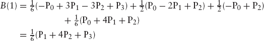
for the first curve segment, based on P0, P1, P2 and P3, while we can immediately see that we obtain exactly this value if we compute B(0) for the second curve segment, based on P1, P2, P3 and P4.
EXERCISES
4.1 Replace the drawLine method based on Bresenham's algorithm and listed near the end of Section 4.1 with an even faster version that benefits from the symmetry of the two halves of the line. For example, with endpoints P and Q satisfying Equation (4.1), and using the integer value xMid halfway between xP and xQ, we can let the variable x run from xp to xMid and also use a variable x2, which at the same time runs backward from xQ to xMid. In each iteration of the loop, x is increased by 1 and x2 is decreased by 1. Note that there will be either one point or two points in the middle of the line, depending on the number of pixels to be plotted being odd or even. Be sure that no pixel of the line is omitted and that no pixel is put twice on the screen. To test the latter, you can use XOR mode so that writing the same pixel twice would have the same effect as omitting a pixel.
4.2 Generalize the method doubleStep2 (of Section 4.2), to make it work for any lines.
4.3 Since normal pixels are very small, they do not show very clearly which of them are selected by Bresenham's algorithms. Use a grid to simulate a screen with a very low resolution. Demonstrate both the method drawLine (with g as its first argument) of Section 4.1 and the method drawCircle of Section 4.3. Only the gridpoints of your grid are to be used as the centers of 'superpixels'. The method putPixel is to draw a small circle with such a center and the distance dGrid of two neighboring gridpoints as its diameter. Do not change the methods drawLine and drawCircle that we have developed, but use dGrid, just mentioned, in a method putPixel that is very different from the one shown at the beginning of Section 4.1. Figure 4.19 shows a grid (with dGrid = 10) and both a line and a circle drawn in this way. As in Figure 4.1, the line shown here has the endpoints P(1, 1) and Q(12, 5) but this time the positive y-axis points downward and the origin is the upper-left corner of the drawing rectangle. The circle has radius r = 8, and is approximated by the same pixels as shown in Figure 4.6 for one eighth of this circle. The line and circle were produced by the following calls to the methods drawLine and drawCircle of Sections 4.1 and 4.3 (but with a different method putPixel):
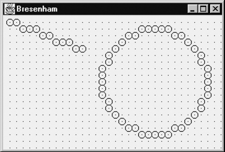
drawLine(g, 1, 1, 12, 5);  // g, xP, yP, xQ, yQ
drawCircle(g, 23, 10, 8);  // g, xC, yC, r
4.4 In the Bezier.java program we constructed only one curve segment, using the points P0, P1, P2 and P3. Extend this program to enable the user to draw very smooth curves consisting of more than one segment. After the first segment has been drawn, the second one is based on these points Q0, Q1, Q2 and Q3 (similar to P0, P1, P2 and P3):
Q0 is identical with P3; clicking on P3 acts as a signal that we want to start another curve segment.
Q1 is not specified by the user, but is automatically constructed by reflecting P2 about P3; in other words, P3 (= Q0) will be the midpoint of P2Q1. This principle will make the curve very smooth.
Q2 and Q3 are defined in the usual way, that is, by clicking on these points.
It should also be possible to specify a third curve segment by starting at Q3, and so on. When the curve (consisting of an arbitrary number of segments) is completed, the user clicks on a point other than the final one of the last segment. This will be the starting point (similar to P0) of an entirely new curve (to be drawn in addition to the previous one), unless, after this, the user clicks on this new point once again: this clicking twice on the same point will be the signal that the drawing is ready. As soon as a curve is completed, it is to be drawn without displaying any straight lines connecting control points and without any little squares marking these points.
4.5 Extend the program Bspline.java of Section 4.7. Supply a grid, with visible gridpoints lying, say, 10 pixels apart, horizontally and vertically. Any control point specified by the user using the mouse should be pulled to the nearest gridpoint. This makes it easier for the user to specify two or more points that lie on the same horizontal or vertical line. Apart from using a grid, your program will also be different from Bspline.java in that it must be able to store several B-spline curves instead of only one. The following characters are to be interpreted as commands:
+ Increase the distance between gridpoints by one.
− Decrease the distance between gridpoints by one.
n After this command, start with a new curve, retaining the previous ones.
d Delete the last curve.
g Change the visibility status of gridpoints (visible/invisible).
c Show only the curves, without any control points or lines connecting these.
4.6 Implement a restricted version of Bresenham's line-drawing algorithm as a demonstration. The purpose of the exercise is to visualize how this algorithm works by showing its stepwise execution on an exaggerated screen area as a 10 × 10 grid. Draw the grid on the left half of the drawing space and the main body of method drawLine2 (listed in Section 4.1) on the right half with text font size of 14. At the bottom of the drawing space, add both a button labeled Step and a small space for displaying the values of the program variables dx, c, m, d, x and y. When the user clicks on two intersection points P and Q, satisfying Equations (4.1), on the grid, a thin line is drawn and the initial values of the program variables d and m are displayed. Just after the definition of point Q, the call to putPixel is highlighted (by coloring or boxing the statement), indicating that this program line is next to be executed. Then whenever the user clicks on Step, the highlighted program line is executed, the next program line in the right half is highlighted, and the values of d, x and y are updated. Each time putPixel is executed, a filled circle is drawn on the appropriate grid intersection (representing a pixel on the line).