Before we proceed with specific computer-graphics subjects, we will discuss some mathematics, which we will often use in this book. You can skip the first four sections of this chapter if you are very familiar with vectors and determinants. After this general part, we will deal with some useful algorithms needed for the exercises at the end of this chapter and for the topics in the remaining chapters. For example, in Chapters 6 and 7 we will deal with polygons that are faces of 3D solid objects. Since polygons in general are difficult to handle, we will divide them into triangles, as we will discuss in the last section of this chapter.
We begin with the mathematical notion of a vector, which should not be confused with the standard class Vector, available in Java to store an arbitrary number of objects. Recall that we have used this Vector class in Section 1.5 to store polygon vertices.
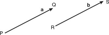
A vector is a directed line segment, characterized by its length and its direction only. Figure 2.1 shows two representations of the same vector a = PQ = b = RS. Thus a vector is not altered by a translation.
The sum c of the vectors a and b, written
c = a + b
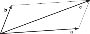
can be obtained as the diagonal of a parallelogram, with a, b and c starting at the same point, as shown in Figure 2.2.
The length of a vector a is denoted by |a|. A vector with zero length is the zero vector, written as 0. The notation –a is used for the vector that has length |a| and whose direction is opposite to that of a. For any vector a and real number c, the vector ca has length |c||a|. If a = 0 or c = 0, then ca = 0; otherwise ca has the direction of a if c > 0 and the opposite direction if c < 0. For any vectors u, v, w and real numbers c, k, we have
| u + v = v + u |
| (u + v) + w = u + (v + w) |
| u + 0 = u |
| u + (-u) = 0 |
| c(u + v) = c u + c v |
| (c + k) u = cu + ku |
| c(ku) = (ck)u |
| 1u = u |
| 0u = 0 |
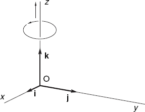
Figure 2.3 shows three unit vectors i, j and k in a three-dimensional space. They are mutually perpendicular and have length 1. Their directions are the positive directions of the coordinate axes. We say that i, j and k form a triple of orthogonal unit vectors. The coordinate system is right-handed, which means that if a rotation of i in the direction of j through 90° corresponds to turning a right-handed screw, then k has the direction in which the screw advances.
We often choose the origin O of the coordinate system as the initial point of all vectors. Any vector v can be written as a linear combination of the unit vectors i, j, and k:
| v = xi + yj + zk |
The real numbers x, y and z are the coordinates of the endpoint P of vector v = OP. We often write this vector v as
| v = (x, y, z) or v = (x, y, z) |
The numbers x, y, z are sometimes called the elements or components of vector v.
The possibility of writing a vector as a sequence of coordinates, such as (x, y, z) for three-dimensional space, has led to the use of this term for sequences in general. This explains the name Vector for a standard Java class. The only aspect this Vector class has in common with the mathematical notion of vector is that both are related to sequences.
The inner product or dot product of two vectors a and b is a real number, written as a · b and defined as
where γ is the angle between a and b. It follows from the first equation that a · b is also zero if γ = 90°. Applying this definition to the unit vectors i, j and k, we find
Setting b = a in Equation (2.1), we have a · a = |a|2, so
Some important properties of inner products are
| c(ku · v) = ck(u · v) |
| (cu + kv) · w = c u · w + kv · w |
| u · v = v · u |
| u · u = 0 only if u = 0 |
The inner product of two vectors u = [u1 u2 u3] and v = [v1 v2 v3] can be computed as
| u · v = u1v1 + u2v2 + u3v3] |
We can prove this by developing the right-hand side of the following equality as the sum of nine inner products and then applying Equation (2.2):
| u · v = (u1 i + u2 j + u3k) · (v1i + v2j + v3k) |
Before proceeding with vector products, we will pay some attention to determinants. Suppose we want to solve the following system of two linear equations for x and y:
We can then multiply the first equation by b2, the second by - b1, and add them, finding
| (a1b2 - a2b1) x = b2c1 - b1c2 |
Then we can multiply the first equation by -a2, the second by a1, and add again, obtaining
| (a1 b2 − a2 b1) y = a1 c2 − a2 c1 |
If a1 b2 − a2 b1 is not zero, we can divide and find
The denominator in these expressions is often written in the form
and then called a determinant. Thus
Using determinants, we can write the solution of Equation (2.3) as
where
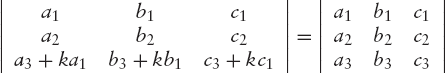
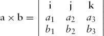
Note that Di is obtained by replacing the ith column of D with the right-hand side of Equation (2.3) (i = 1 or 2). This method of solving a system of linear equations is called Cramer's rule. It is not restricted to systems of two equations (although it would be very expensive in terms of computer time to apply the method to large systems). Determinants with n rows and n columns are said to be of the nth order. We define determinants of third order by using the equation
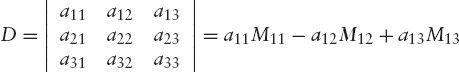
where each so-called minor determinant Mij is the 2 × 2 determinant that we obtain by deleting the ith row and the jth column of D. Determinants of higher order are defined similarly.
Determinants are very useful in linear algebra and analytical geometry. They have many interesting properties, some of which are listed below:
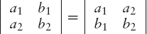
The value of a determinant remains the same if its rows are written as columns in the same order. For example:
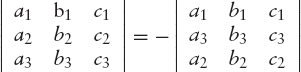
If any two rows (or columns) are interchanged, the value of the determinant is multiplied by – 1. For example:
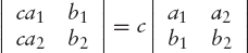
If any row or column is multiplied by a factor, the value of the determinant is multiplied by this factor. For example:
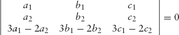
If a row is altered by adding any constant multiple of any other row to it, the value of the determinant remains unaltered. This operation may also be applied to columns. For example:
If a row (or a column) is a linear combination of some other rows (or columns), the value of the determinant is zero. For example:
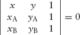
In many cases, determinant equations expressing geometrical properties are elegant and easy to remember. For example, the equation of the line in R2 through the two points P1(x1, y1) and P2(x2, y2) can be written
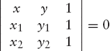
This can be understood by observing, first, that Equation (2.5) is a special notation for a linear equation in x and y, and consequently represents a straight line in R2, and second, that the coordinates of both P1 and P2 satisfy this equation, for if we write them in the first row, we have two identical rows. Similarly, the plane in R3 through three points P1(x1, y1, z1), P2(x2, y2, z2), P3(x3, y3, z3) has the equation
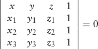
which is much easier to remember than one written in the conventional way.
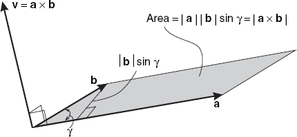
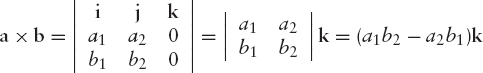
The vector product or cross product of two vectors a and b is written
| a × b |
and is a vector v with the following properties. If a = cb for some scalar c, then v = 0. Otherwise the length of v is equal to
| |v| = |a||b| sin γ |
where γ is the angle between a and b, and the direction of v is perpendicular to both a and b and is such that a, b and v, in that order, form a right-handed triple. This means that if a is rotated through an angle γ < 180° in the direction of b, then v has the direction of the advancement of a right-handed screw if turned in the same way. Note that the length |v| is equal to the area of a parallelogram of which the vectors a and b can act as edges, as Figure 2.4 shows.
The following properties of vector products follow from this definition:
| (ka) × b = k(a × b) for any real number k |
| a × (b + c) = a × b + a × c |
| a × b = -b × a |
In general, a × (b × c) ≠ (a × b) × c. If we apply our definition of vector product to the unit vectors i, j, k (see Figure 2.3), we have
| i × i = 0 j × j = 0 k × k = 0 |
| i × j = k j × k = i k × i = j |
| j × i = −k k × j} = −i i × k = −j |
Using these vector products in the expansion of
| a × b = (a1i + a2j + a3k) × (b1i + b2j + b3k) |
we obtain
| a × b = (a2b3 − a3b2)i + (a3b1 − a1b3)j + (a1b2 − a2b1)k |
which can be written as
We rewrite this in a form that is very easy to remember:
This is a mnemonic aid rather than a true determinant, since the elements of the first row are vectors instead of numbers.
If a and b are neighboring sides of a parallelogram, as shown in Figure 2.4, the area of this parallelogram is the length of vector a × b. This follows from our definition of vector product, according to which |a × b| = |a||b| sin γ is the length of vector a × b.
We will now deal with a subject that will be very useful in Chapters 6 and 7. Suppose that we are given an ordered triple (A, B, C) of three points in the xy-plane and we want to know their orientation; in other words, we want to know whether we turn counter-clockwise or clockwise when visiting these points in the given order. Figure 2.5 shows the possibilities, which we also refer to as positive and negative orientation, respectively.
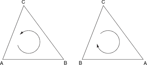
There is a third possibility, namely that the points A, B and C lie on a straight line. We will consider the orientation to be zero in this case. If we plot the points on paper, we see immediately which of these three cases applies, but we now want a means to find the orientation by computation, using only the coordinates xA, yA, xB, yB, xC, yC.
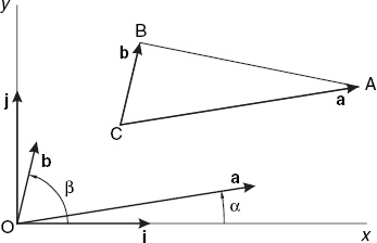
Let us define the two vectors a = CA and b = CB, as shown in Figure 2.6. Clearly, the orientation of the original points A, B and C is positive if we can turn the vector a counter-clockwise through a positive angle less than 180° to obtain the direction of the vector b. Since vectors are only determined by their directions and lengths, we may let them start at the origin O instead of at point C, as Figure 2.6 shows. Although this orientation problem is essentially two-dimensional, and can be solved using only 2D concepts, as we will see in a moment, it is convenient to use 3D space. As usual, the unit vectors i, j and k have the directions of the positive x-, y- and z-axes. In Figure 2.6, we imagine the vector k, like i and j starting at O, and pointing towards us. Denoting the endpoints of the translated vectors a and b, starting at O, by (a1, a2, 0) and (b1, b2, 0), we have
| a = a1i + a2j + 0k |
| b = b1i + b2j + 0k |
and
This expresses the fact that a × b is a vector perpendicular to the xy-plane and either in the same direction as
| k = i × j |
or in the opposite direction, depending on the sign of a1b2 - a2b1. If this expression is positive, the relationship between a and b is similar to that of i and j: we can turn a counter-clockwise through an angle less than 180° to obtain the direction of b, in the same way as we can do this with i to obtain j. In general, we have
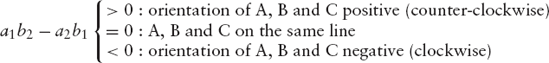
It would be unsatisfactory if we were unable to solve the above orientation problem by using only two-dimensional concepts. To provide such an alternative solution, we use the angles α between vector a and the positive x-axis and β between b and this axis (see Figure 2.6). Then the orientation we are interested in depends upon the angle β – α. If this angle lies between 0 and π, the orientation is clearly positive, but it is negative if this angle lies between π and 2π (or between -π and 0). We can express this by saying that the orientation in question depends on the value of sin(β – α) rather than on the angle β – α itself. More specifically, the orientation has the same sign as
Since the denominator in this expression is the product of two vector lengths, it is positive, so that we have again found that the orientation of A, B and C and a1b2 – a2b1 have the same sign. Due to unfamiliarity with the above trigonometric formula, some readers may find the former, more visual 3D approach easier to remember.
The method area2 in the following fragment is based on the results we have found. This method takes three arguments of class Point2D, discussed at the end of Chapter 1. We will use the class Tools2D for several static methods, to be used as two-dimensional tools (see also Section 2.13). Note that, in accordance with Java convention, we use lower-case variable names a, b, c for the points A, B and C:
class Tools2D
{   static float area2(Point2D a, Point2D b, Point2D c)
    {  return (a.x – c.x) * (b.y – c.y) – (a.y – c.y) * (b.x – c.x);
    }
    ... // See Section 2.13
}
As we will see in Section 2.7, this method computes the area of the triangle ABC multiplied by 2, or, if A, B and C are clockwise, by −2. If we are interested only in the orientation of the points A, B and C, each of type Point2D, we can write:
if (Tools2D.area2(a, b, c) > 0)
{  ... // A, B and C counter-clockwise
}
else
{  ...
// A, B and C clockwise (unless the area2 method return 0; // in that case A, B and C lie on the same line). }
A polygon is a sequence P0, P1, ..., Pn−1 of vertices, where n≥3, with associated edges P0P1, P1P2, ..., Pn– 2Pn–1,Pn–1,P0. In this book we will restrict ourselves to simple polygons, of which non-adjacent edges do not intersect. Figure 2.7 shows two simple and two non-simple polygons, for all of which n = 5.
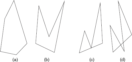
Besides non-simple polygons, such as those in Figure 2.7(c) and (d), we usually also ignore polygons in which three successive vertices lie on the same line. A vertex of a polygon is said to be convex if the interior angle between the two edges meeting at that vertex is less than 180°. If all vertices of a polygon are convex, the polygon itself is said to be convex, as is the case with Figure 2.7(a). Non-convex vertices are referred to as reflex. If a polygon has at least one reflex vertex, the polygon is said to be concave. Figure 2.7(b) shows a concave polygon because the vertex in the middle is reflex. All triangles are convex, and each polygon has at least three convex vertices.
If we are given the vertices P0, P1, ..., Pn–1 of a polygon, it may be desirable to determine whether this vertex sequence is counter-clockwise. If we know that the second vertex, P1, is convex, we can simply write
if (Tools2D.area2(p[0], p[1], p[2]) > 0)
   ... // Counter-clockwise
else
   ... // Clockwise
The problem is more interesting if no information about any convex vertex is available. We then have to detect such a vertex. This is an easy task, since any vertex whose x- or y-coordinate is extreme is convex. For example, we can use a vertex whose x-coordinate is not greater than that of any other vertex. If we do not want to exclude the case of three successive vertices lying on the same line, we must pay special attention to the case of three such vertices having the minimum x-coordinate. Therefore, among all vertices with an x-coordinate equal to this minimum value, we choose the lowest one, that is, the one with the least y-coordinate. The following method is based on this idea:
static boolean ccw(Point2D[] p)
{  int n = p.length, k = 0;
   for (int i=1; i<n; i++)
      if (p[i].x <= p[k].x && (p[i].x < p[k].x || p[i].y < p[k].y))
         k = i;
   // p[k] is a convex vertex.
   int prev = k − 1, next = k + 1;
   if (prev == −1) prev = n − 1;
   if (next == n) next = 0;
   return Tools2D.area2(p[prev], p[k], p[next]) > 0;
}
We should be aware that one very strange situation is still possible: all n vertices may lie on the same line. In that case, the method ccw will return the value false.
We will use this method in Section 2.13, in which program PolyTria.java will divide a user-entered polygon into triangles.
As we have seen in Figure 2.4, the cross product a × b is a vector whose length is equal to the area of a parallelogram of which a and b are two edges. Since this parallelogram is the sum of two triangles of equal area, it follows that for Figure 2.6 we have
Note that this is valid only if A, B and C are labeled counter-clockwise; if this is not necessarily the case, we have to use the absolute value of a1b2 – a2b1.
| Since a1 = xA – xC, a2 = yA – yC, b1 = xB – xC, b2 = yB – yC, we can also write |
| 2 Area(ΔABC) = (xA – xC)(yB – yC) – (yA – yC)(xB – xC) |
After working this out, we find that we can replace this with
| 2 Area(ΔABC) = (xAyB – yAxB) + (xByC – yBxC) + (xCyA – yCxA) |
Although the latter expression seems hardly an improvement, it is useful to prepare for a more general one, which we can use to compute the area of any polygon, convex or concave, which has the vertices P0P1, P1P2, ..., Pn – 2Pn–1, Pn–1, labeled counter-clockwise:
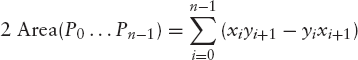
where (xi, yi) are the coordinates of Pi and Pn is the same vertex as P0. As you can see, our last formula for the area of a triangle is a special case of this general one, in which the area of a polygon is expressed directly in terms of the coordinates of its vertices. A complete proof of this formula is beyond the scope of this book.
As we have seen in Section 2.6, we use the method area2 to determine the orientation of three points A, B and C. Recall that the digit 2 in the name area2 indicates that we have to divide the return value by 2 to obtain the area of triangle ABC, that is, if A, B and C are counter-clockwise; otherwise, we have to take the absolute value |area2(A, B, C)/2|.
The same applies to the following method area2, whose return value divided by 2 gives the area, possibly preceded by a minus sign, of a polygon.
static float area2(Point2D[] pol)
{  int n = pol.length,
       j = n – 1;
   float a = 0;

   for (int i=0; i<n; i++)
   {  // i and j denote neighbor vertices
      // with i one step ahead of j
      a += pol[j].x * pol[i].y – pol[j].y * pol[i].x;
      j = i;
   }
   return a;
}
Note that this second area2 method provides another means of deciding the orientation of a polygon vertex sequence: this orientation is counter-clockwise if area2 returns a positive value and clockwise if it returns a negative one. However, the method ccw discussed in Section 2.6 is faster, especially if n is large, because for most vertices it will only perform the comparison
p[i].x <= p[k].x
while area2 performs some more time-consuming arithmetic operations for each vertex.
We could add this second method area2 to the class Tools2D, but you will not find it in our final version of this class in Section 2.13 because we will never use it in this book; since we will use Tools2D several times, we prefer to omit superfluous methods for economic reasons.
Determining the orientation of three points as we have just been discussing is useful in a test to see if a given point P lies within a triangle ABC. As Figure 2.8 shows, this is the case if the orientation of the triangles ABP, BCP and CAP is the same as that of triangle ABC.
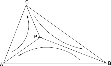
Let us assume that we know that the orientation of ABC is counter-clockwise. We can then call the following method to test if P lies within triangle ABC (or on an edge of it):
static boolean insideTriangle(Point2D a, Point2D b, Point2D c,
   Point2D p) // ABC is assumed to be counter-clockwise
{  return
Tools2D.area2(a, b, p) >= 0 &&
Tools2D.area2(b, c, p) >= 0 &&
Tools2D.area2(c, a, p) >= 0;
}In this form, the method insideTriangle also returns the value true if P lies on an edge of the triangle ABC. If this is not desired, we should replace >= 0 with >0. The above form is the one we will need in Chapters 6 and 7, in which we will use this method to triangulate complicated polygonal faces of 3D objects.
Incidentally, with a floating-point value x, we might consider replacing a test of the form x >= 0 with x >= – epsilon and x > 0 with x > epsilon, where epsilon is some small positive value, such as 10−6. In this way a very small rounding-off error (less than epsilon) in the value of x will not affect the result of the test. This is not done here because the above method insideTriangle works well for our applications.
The above method insideTriangle is reasonably efficient, especially if point P does not lie within the triangle ABC. In such cases the chances are that not all three calls to area2 are executed because the first or the second of the three tests fails. However, it should be mentioned that there is an entirely different way of solving the problem in question, as we will see in Exercise 3.5. The corresponding alternative method insideTriangle (listed in Appendix F), is slightly faster than the one above if a single triangle ABC is to be used for several points P. It is also more general in that it does not rely on ABC being counter-clockwise. We will not discuss this alternative method here because it is easier to understand after the discussion of matrix multiplication and inverse matrices in Chapter 3. To avoid confusion we will normally use the insideTriangle version discussed in this section and occurring in the file Tools2D.java, even in cases where the one in Exercise 3.5 might be slightly faster.
The notion of orientation is also useful when we need to determine whether a given point P lies within a polygon. It will then be convenient if a method is available which accepts both the polygon in question and point P as arguments, and returns true if P lies inside and false if it lies outside the polygon. If P lies on a polygon edge, we do not care: in that case the method may return true or false. The method we will discuss is based on the idea of drawing a horizontal half-line, which starts at P and extends only to the right. The number of intersections of this horizontal half-line with polygon edges is odd if P lies within the polygon and even if P lies outside it. Imagine that we move to the right, starting at point P. Then our state changes from inside to outside and vice versa each time we cross a polygon edge. The total number of changes is therefore odd if P lies within the polygon and even if it lies outside the polygon. It is not necessary to visit all intersections strictly from left to right; the only thing we want to know is whether there are an odd or an even number of intersections on a horizontal line through P and to the right of P. However, we must be careful with some special cases, as shown in Figure 2.9.
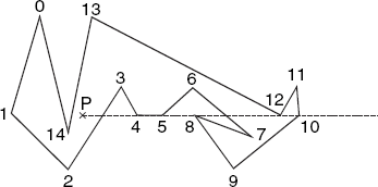
We simply ignore horizontal polygon edges, even if they have the same y-coordinate as P, as is the case with edge 4–5 in this example. If a vertex occurring as a 'local maximum or minimum' happens to have the same y-coordinate as P, as is the cases with vertices 8 and 12 in this example, it is essential that this is either ignored or counted twice. We can realize this by using the edge from vertex i to vertex i + 1 only if
| yi ≤ yP < yi + 1 or yi + 1 ≤ yP < yi |
This implies that the lower endpoint of a non-horizontal edge is regarded as part of the segment, but the upper endpoint is not. For example, in Figure 2.9, vertex 8 (with y8 = yP) is not counted at all because it is the upper endpoint of both edge 7–8 and edge 8–9. By contrast, vertex 12 (with y12 = yP) is the lower endpoint of the edges 11–12 and 12–13 and thus counted twice. Therefore, in this example, we count the intersections of the half-line through P with the seven edges 2–3, 3–4, 5–6, 6–7, 10–11, 11–12, 12–13 and with no others.
Since we are considering only a half-line, we must impose another restriction on the set of edges satisfying the above test, selecting only those whose point of intersection with the half-line lies to the right of P. One way of doing this is by using the method area2 to determine the orientation of a sequence of three points. For example, this orientation is counter-clockwise for the triangle 2-3-P in Figure 2.9, which implies that P lies to the left of edge 2–3. It is also counter-clockwise for the triangle 7-6-P. In both cases, the lower endpoint of an edge, its upper endpoint and point P, in that order, are counter-clockwise. The following method is based on these principles:
static boolean insidePolygon(Point2D p, Point2D[] pol)
{ int n = pol.length, j = n – 1;
boolean b = false;
float x = p.x, y = p.y;
for (int i=0; i<n; i++)
{ if (pol[j].y <= y && y < pol[i].y &&
Tools2D.area2(pol[j], pol[i], p) > 0 ||
pol[i].y <= y && y < pol[j].y &&
Tools2D.area2(pol[i], pol[j], p) > 0) b = !b;
j = i;
}
return b;
}This static method, like some others in this chapter, might be added to the class Tools2D (see Section 2.13).
There is a standard class Polygon, which has a member named contains to perform about the same task as the above method insidePolygon. However, it is based on integer coordinates.
For example, to test if a point P(xP, yP) lies within the triangle with vertices A(20, 15), B(100, 30) and C(80, 150), we can use the following fragment:
int[] x = {20, 100, 80}, y = {15, 30, 150}; // A, B, C
Polygon p = new Polygon(x, y, 3);
if (p.contains(xP, yP)) ... // P lies within triangle ABC.If P lies exactly on a polygon edge, the value returned by this method contains of the class Polygon can be true or false.
Testing whether a point P lies on a given line is very simple if this line is given as an equation, say,
Then all we need to do is to test whether the coordinates of P satisfy this equation. Due to inexact computations, such a test may fail when it should succeed. It may therefore be wise to be slightly more tolerant, so that we might write
if (Math.abs(a * p.x + b * p.y – h) < eps) // P on the line
where eps is some small positive value, such as 10−5.
If the line is not given by an equation but by two points A and B on it, we can use the above test after deriving an equation for the line, as discussed in Section 2.3, writing
which gives the following coefficients for Equation (2.7):
| a = yA — yB |
| b = xB — xA |
| h = xByA — xAyB |
Instead, we can benefit from the area2 method, which we are now familiar with. After all, if and only if P lies on the line through A and B, the triangle ABP is degenerated and has a zero area. We can therefore write
if (Math.abs(Tools2D.area2(a, b, p)) < eps) // P on line AB
Again, if we simply test whether the computed area is equal to zero, such a test might fail when it should succeed, due to rounding-off errors.
If three points A, B and P are given, we may want to determine whether P lies on the closed line segment AB. The adjective closed here means that we include the endpoints A and B, so that the question is to be answered affirmatively if P lies between A and B or coincides with one of these points. We assume that A and B are different points, which implies that xA ≠ xB or yA ≠ yB. If xA ≠ xB we test whether xP lies between xA and xB; if not, we test whether yp lies between yA and yB, where in both cases the word between includes the points A and B themselves. This test is sufficient if it is given that P lies on the infinite line AB. If that is not given, we also have to perform the above test, which is done in the following method:
static boolean onSegment(Point2D a, Point2D b, Point2D p)
{ double dx = b.x – a.x, dy = b.y – a.y,eps = 0.001 * (dx * dx + dy * dy);
return
(a.x != b.x &&
(a.x <= p.x && p.x <= b.x || b.x <= p.x && p.x <= a.x)
|| a.x == b.x &&
(a.y <= p.y && p.y <= b.y || b.y <= p.y && p.y <= a.y))
&& Math.abs(Tools2D.area2(a, b, p)) < eps;
}The expression following return relies on the operator && having higher precedence than ||. Since both operators && and || evaluate the second operand only if this is necessary, this test is more efficient than it looks. For example, if xA ≠ xB the test on the line of the form (a.y <= ...) is not evaluated at all. The positive constant eps in the above code has been chosen in such a way that the area of triangle ABP is compared with a fraction of another area, for which the square of side AB is used. In this way, the compared areas depend in the same way on both the length of AB and the unit of length that is used.
Instead of testing if P lies on the segment AB, we may want to apply a similar test to the projection P′ of P on AB, as Figure 2.10 shows.
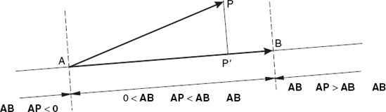
We can solve this problem by computing the dot product of the vectors AB and AP. This dot product AB · AP is equal to 0 if P′ ≡ A (P′ coincides with A) and it is equal to AB · AB = AB2 if P′ ≡ B. For any value of this dot product between these two values, P lies between A and B. We can write this as follows in a program, where len2 corresponds to AB · AB, inprod corresponds to AB · AP, and eps is some small positive value, as discussed for the above method onSegment:
// Does Pstquote (P projected on AB) lie on the closed segment AB?
static boolean projOnSegment(Point2D a, Point2D b, Point2D p)
{ double dx = b.x - a.x, dy = b.y - a.y,eps = 0.001 * (dx * dx + dy * dy),
len2 = dx * dx + dy * dy,
inprod = dx * (p.x - a.x) + dy * (p.y - a.y);
return inprod > -eps && inprod < len2 + eps;
}To determine whether P′ lies on the open segment AB (not including A and B), we replace the return statement with
return inprod > eps && inprod < len2 – eps;
We can find the distance between a point P and a line l in different ways, depending on the way the line is specified. If two points A and B of the line are given, we can find the distance between a point P and the (infinite) line l through A and B by using the first of the two methods area2 defined in Section 2.7:
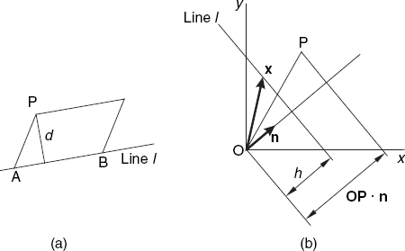
This follows from the fact that the absolute value of area2(A, B, P) denotes the area of the parallelogram of which A, B and P are three vertices, as shown in Figure 2.11(a). This area is also equal to the product of the parallelogram's base AB and its height d. We can therefore compute d in the above way.
If the line l is given as an equation, we assume this to be in the form
| ax + by = h |
where
If the latter condition is not satisfied, we only have to divide a,b and h by the above square root. We can then write the above equation of line l as the dot product
| x·n = h |
where
The normal vector n is perpendicular to line l and has length 1. For any vector x, starting at O, the dot product x · n is the projection of vector x on n. This also applies if the endpoint of x lies on line l, as shown in Figure 2.11(b); in this case we have x · n = h. We find the desired distance between point P and line l by projecting OP also on n and computing the difference of the two projections:
| Distance between P and line l = |OP·n – h| = |axp + byp – h| |
Although Figure 2.11(b) applies to the case h > 0, this equation is also valid if h is negative or zero, or if O lies between line l and the line through P parallel to l. Both OP · n and h are scale factors for the same vector n. The absolute value of the algebraic difference of these two scale factors is the desired distance between P and l. We will refer to this algebraic difference OP · n – h = axp + byp – h as a signed distance in the next section.
Suppose that again a line l and a point P (not on l) are given and that we want to compute the projection P′ of P on l (see Figure 2.10). This point P′ has three interesting properties:
P′ is the point on l that is closest to P.
The length of PP′ is the distance between P and l (computed in the previous section).
PP′ and l are perpendicular.
As in the previous section, we discuss two solutions: one for a line l given by two points A and B, and the other for l given as the equation x · n = h.
With given points A and B on line l, the situation is as shown in Figure 2.10. Recall that in Section 2.10 we discussed the method projOnSegment to test if the projection P′ of P on the line through A and B lies between A and B. In that method, we did not actually compute the position of P′. We will now do this (see Figure 2.10), first by introducing the vector u of length 1 and direction AB:
Then the length of the projection AP′ of AP is equal to
| λ = AP · u |
which we use to compute
| AP′ = λ u |
Doing this straightforwardly would require a square-root operation in the computation of the distance between A and B, used in the computation of u. Fortunately, we can avoid this by rewriting the last equation, using the two preceding ones:
The advantage of the last form is that the square of the segment length AB is easier to compute than that length itself. The following method, which returns the projection P′ of P on AB, demonstrates this:
// Compute Pstquote (P projected on AB):
static Point2D projection(Point2D a, Point2D b, Point2D p)
{ float vx = b.x - a.x, vy = b.y - a.y, len2 = vx * vx + vy * vy,
inprod = vx * (p.x - a.x) + vy * (p.y - a.y);
return new Point2D(a.x + inprod * vx/len2,
a.y + inprod * vy/len2);
}So much for a line given by two points A and B.
Let us now turn to a line l given by its equation, which we again write as
| x · n = h |
where
and
Using the 'signed distance'
| d = OP · n – h |
as introduced at the end of the previous section and illustrated by Figure 2.11, we can write the following vector equation to compute the desired projection P′ of P on l:
This should make the following method clear:
// Compute Pstquote, the projection of P on line l given as
// ax + by = h, where a * a + b * b = 1
static Point2D projection(float a, float b, float h,
Point2D p)
{ float d = p.x * a + p.y * b - h;
return new Point2D(p.x - d * a, p.y - d * b);
}In many graphics applications, such as those to be discussed in Chapters 6 and 7, it is desirable to divide a polygon into triangles. This triangulation problem can be solved in many ways. We will discuss a comparatively simple algorithm. It accepts a polygon in the form of an array of Point2D elements (see Section 1.5), containing the polygon vertices in counter-clockwise order. The triangulate method that we will discuss takes such an array as an argument. To store the resulting triangles, it also takes a second argument, an array with elements of type Triangle, which is defined as follows:
// Triangle.java: Class to store a triangle;
// vertices in logical coordinates.
// Uses: Point2D (Section 1.5).
class Triangle
{ Point2D a, b, c;
Triangle(Point2D a, Point2D b, Point2D c)
{ this.a = a; this.b = b; this.c = c;
}
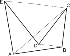
}If the given polygon has n vertices, this triangle array should have length n – 2. The algorithm works as follows. Traversing the vertices of the polygon in counter-clockwise order, for every three successive vertices P, Q and R of which Q is a convex vertex (with an angle less than 180°), we cut the triangle PQR off the polygon if this triangle does not contain any of the other polygon vertices. For example, starting with polygon ABCDE in Figure 2.12, we cannot cut triangle ABC, because this contains vertex D. Nor is triangle CDE a good candidate, because D is not a convex vertex. There are no such problems with triangle BCD, so that we will cut this off the polygon, reducing the polygon ABCDE to the simpler one ABDE.
For this purpose we use the static method triangulate, which, along with some others already discussed, is listed in the class Tools2D below:
// Tools2D.java: Class to be used in other program files.
// Uses: Point2D (Section 1.5) and Triangle (discussed above).
class Tools2D
{ static float area2(Point2D a, Point2D b, Point2D c)
{ return (a.x - c.x) * (b.y - c.y) - (a.y - c.y) * (b.x - c.x);
}
static boolean insideTriangle(Point2D a, Point2D b, Point2D c,
Point2D p) // ABC is assumed to be counter-clockwise
{ return
Tools2D.area2(a, b, p) >= 0 &&
      Tools2D.area2(b, c, p) >= 0 &&
      Tools2D.area2(c, a, p) >= 0;
}
static void triangulate(Point2D[] p, Triangle[] tr)
{ // p contains all n polygon vertices in CCW order.// The resulting triangles will be stored in array tr.
// This array tr must have length n − 2.
int n = p.length, j = n − 1, iA=0, iB, iC;
int[] next = new int[n];
for (int i=0; i<n; i++)
{ next[j] = i;
j = i;
}
for (int k=0; k<n-2; k++)
{ // Find a suitable triangle, consisting of two edges
// and an internal diagonal:
Point2D a, b, c;
boolean triaFound = false;
int count = 0;
while (!triaFound && ++count < n)
{ iB = next[iA]; iC = next[iB];
a = p[iA]; b = p[iB]; c = p[iC];
if (Tools2D.area2(a, b, c) >= 0)
{ // Edges AB and BC; diagonal AC.
// Test to see if no other polygon vertex
// lies within triangle ABC:
j = next[iC];
while (j != iA && !insideTriangle(a, b, c, p[j]))
j = next[j];
if (j == iA)
{ // Triangle ABC contains no other vertex:
tr[k] = new Triangle(a, b, c);
next[iA] = iC;
triaFound = true;
}
}
iA = next[iA];
}
if (count == n)
{ System.out.println("Not a simple polygon" +
" or vertex sequence not counter-clockwise.");
System.exit(1);
}
}
}
static float distance2(Point2D p, Point2D q)
{ float dx = p.x - q.x,dy = p.y - q.y;
return dx * dx + dy * dy;
}
}In Appendix D we will use the method distance2, shown at the end of this class; it simply computes the square of the distance of two points P and Q. If we only want to compare two distances, we may as well compare their squares to save the rather costly operation of computing the square roots.
The program below enables the user to define a polygon, in the same way as we did with program DefPoly.java in Section 1.5, but this time the polygon will be divided into triangles, which appear in different colors. This program, PolyTria.java, uses the above classes Triangle and Tools2D, as well as the class CvDefPoly, which occurs in program DefPoly.java of Section 1.5. In our subclass, CvPolyTria, we apply the method ccw, discussed in Section 2.6, to the given polygon to examine the orientation of its vertex sequence. If this happens to be clockwise, we put the vertices in reverse order in the array P, so that the vertex sequence will be counter-clockwise in this array, which we can then safely pass on to the triangulate method:
// PolyTria.java: Drawing a polygon and dividing it into triangles.
// Uses: CvDefPoly, Point2D (Section 1.5),
//       Triangle, Tools2D (discussed above).

import java.awt.*;
import java.awt.event.*;
import java.util.*;
public class PolyTria extends Frame
{  public static void main(String[] args){new PolyTria();}

   PolyTria()
   {  super("Define polygon vertices by clicking");
      addWindowListener(new WindowAdapter()
         {public void windowClosing(WindowEvent e){System.exit(0);}});
      setSize (500, 300);
      add("Center", new CvPolyTria());

   setCursor(Cursor.getPredefinedCursor(Cursor.CROSSHAIR_CURSOR));
         show();
   }
}
class CvPolyTria extends CvDefPoly // see Section 1.5
{ public void paint(Graphics g)
{ int n = v.size();
if (n > 3 && ready)
{ Point2D[] p = new Point2D[n];
for (int i=0; i<n; i++) p[i] = (Point2D)v.elementAt(i);
// If not counter-clockwise, reverse the order:
if (!ccw(p))
for (int i=0; i<n; i++)
p[i] = (Point2D)v.elementAt(n − i - 1);
int ntr = n − 2;
Triangle[] tr = new Triangle[ntr];
Tools2D.triangulate(p, tr);
initgr();
for (int j=0; j<ntr; j++)
{ g.setColor(new Color(rand(), rand(), rand()));
int[] x = new int[3], y = new int[3];
x[0] = iX(tr[j].a.x); y[0] = iY(tr[j].a.y);
x[1] = iX(tr[j].b.x); y[1] = iY(tr[j].b.y);
x[2] = iX(tr[j].c.x); y[2] = iY(tr[j].c.y);
g.fillPolygon(x, y, 3);
}
}
g.setColor(Color.black);
super.paint(g);
}
int rand(){return (int)(Math.random() * 256);}
static boolean ccw(Point2D[] p)
{ int n = p.length, k = 0;
for (int i=1; i<n; i++)
if (p[i].x <= p[k].x && (p[i].x < p[k].x || p[i].y < p[k].y))
k = i;
// p[k] is a convex vertex.
int prev = k – 1, next = k + 1;
if (prev == −1) prev = n – 1;
if (next == n) next = 0;
return Tools2D.area2(p[prev], p[k], p[next]) > 0;
}
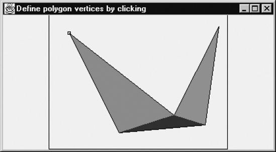
}The canvas class CvPolyTria is a subclass of CvDefPoly so that the construction of a polygon with vertices specified by the user is done in the same way as in Section 1.5. In this subclass, we call the method triangulate to construct the array tr of triangles. These are then displayed in colors generated with a random number generator, so that we can clearly distinguish them. The result on the screen is much better than Figure 2.13, because the latter shows only shades of gray instead of the real colors.
EXERCISES
2.1 Write a program that draws a square ABCD. The points A and B are arbitrarily specified by the user by clicking the mouse button. The orientation of the points A, B, C and D should be counter-clockwise.
2.2 Write a program that, for four points A, B, C and P,
draws a triangle formed by ABC and a small cross showing the position of P; and
displays a line of text indicating which of the following three cases applies: P lies (a) inside ABC, (b) outside ABC, or (c) on an edge of ABC.
The user will specify the four points by clicking.
2.3 The same as Exercise 2.2, but, instead of displaying a line of text, the program computes the distances from P to the (infinite) lines AB, BC and CA, and draws the shortest possible line that connects P with the nearest of those three lines.
2.4 Write a program that computes the intersection point of two (infinite) lines AB and CD. The user will specify the points A, B, C and D by clicking. Draw a small circle around the intersection point. If the two lines AB and CD do not have a unique intersection point (because they are parallel or coinciding), display a line of text indicating this.
2.4 Write a program that constructs the bisector of the angle ABC (which divides the angle at B into two equal angles). After the user has specified the points A, B and C by clicking, the program should compute the intersection point D of this bisector with the opposite side AC, and draw both triangle ABC and bisector BD.
2.5 Write a program that draws the circumscribed circle (also known as the circumcircle) of a given triangle ABC; this circle passes through the points A, B and C. These points will be specified by the user by clicking the mouse button. Remember, the three perpendicular bisectors of the three edges of a triangle all pass through one point, the circumcenter, which is the center of the circumscribed circle.
2.7 Write a program that, for three given points P, Q and R specified by the user, draws a circular arc, starting at P, passing through Q and ending at R (see also Exercise 2.6).
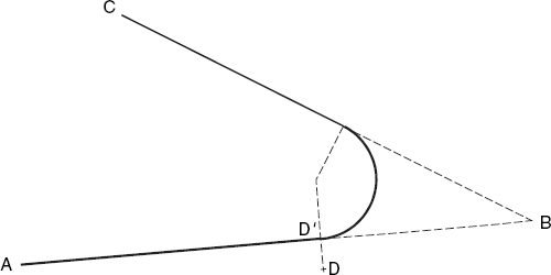
2.8 Construct a fillet to replace a sharp corner with a rounded one, as illustrated by the solid lines and the arc in Figure 2.14. The four points A, B, C and D are specified by the user by clicking. Point D may or may not lie on AB; if it does not, it is projected onto AB, giving D′, as Figure 2.14 illustrates. The arc starts at point D′.
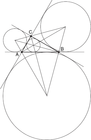
2.9 Construct the inscribed circle (or incircle) of a given triangle ABC. The center of this circle lies on the point of intersection of the (internal) bisectors of the three angles A, B and C. Draw also the three excircles, which, like the incircle, are tangent to the sides of the triangle, as shown in Fig. 2.15. The centers of the excircles lie on the points of intersection of the external bisectors of the angles A, B and C.
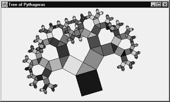
2.10 Write a program that draws a tree of Pythagoras as shown in Figure 2.16. Two vertices A and B, the basis of the tree, are specified by the user by clicking. Then both a square ABCD and an isosceles,
right-angled triangle DCE, with right angle E, are constructed. The orientation of both ABCD and DCE is counter-clockwise. Finally, the points D and E form the basis of another tree of Pythagoras, and so do the points E and C. Use a recursive method, which does nothing at all if the two supplied basis points are closer together than some limit.