Chapter 7

Advanced Control of the Linear Synchronous Motor ¹

7.1. Introduction

This chapter presents some advanced controls of the permanent magnet linear synchronous motor (PMLSM). In section 7.1.1 we present a short historical and general introduction of this type of motor. We take a short look at state-of-the-art PMLSM technology in industry at present.

In section 7.2.1, we propose a brief overview of state-of-the-art of industrial controls available for linear synchronous motors. Then, advanced controls specific for linear motors are presented.

In particular in this chapter, control design is elaborated using the causal ordering graph (COG) principle that is applied to advanced analytical models of PMLSM, including cogging forces and end-effect forces. The COG principle facilitates the analysis of the physical model for controller tuning. Some advanced controls are presented, including estimator and feed-forward control, resonant controller and the nth derivative of the control variables in open-loop control.

7.1.1. Historical review and applications in the field of linear motors

One of the first transportation designs using linear motors was patented more than a century ago. It was designed by Alfred Zehden and patented in Switzerland in 1902 [ZEH 02] and in the US in 1905. The patents focus on the use of linear induction motors (LIMs) to move passenger trains. In such an application, the primary was fixed by sections on top of a rail, along the railway. Each section successively received the power supply, allowing the train to move forward. The high fabrication cost of the rail, however, put an end to the development of this electric propulsion device.

The market in industrial applications using PMLSMs has only taken off since the end of the 1980s [MCL 88] with constant growth to date [EAS 02]. To understand such success, it is important to remember that industry has always tried to find solutions to reduce manufacturing time and to be very flexible. To achieve this, engineers have used agile machines, focusing on cheap and very simple concepts, recognized as the “lean” production practice that leads to lightening structures to adapt to the problem of size alone. In such a concept, LIMs have naturally become a vital component.

In 2004, the European and American markets for LIMs were worth €113 million ($153,000,000) and €95 million ($128,000,000) respectively [GIE 03]. It is a sector in full expansion, which is venturing into new fields of applications. Nevertheless, there is currently no mass market for linear motors. The business only survives due to innovations and the inventiveness of the applications. [CAS 03] presents a synthesis of the main applications of linear synchronous motors. Among them, we can find: the electromagnetic cannon, the magnetic levitation train (see Figure 7.1a), roller-coasters, ropeless elevators, conveyor belts, robotics, machine-tools, world-class high-accuracy positioning systems for the electronic and semiconductor industries (see Figure 7.1b).

7.1.2. Presentation of linear synchronous motors

A linear motor is used to move a system without any additional kinematic components in a linear translation1 . Figure 7.2 presents a PMLSM. It can be classified as a flat, single-sided, slotted, short primary and iron-core LSM:

– a primary, lightweight moving part composed of a three-phase coil and a laminated stack used as a ferromagnetic circuit;

– a secondary, fixed part composed of a permanent magnet lying on a ferromagnetic yoke.

In a classical transmission device, the high number of mechanical linkages introduces flexibility, torsion and flexion of the screw, backlash, vibration, etc. For example, accuracy and repeatability suffer from the inherent limitations of the moving belt system. Therefore the limit on the positioning accuracy and high dynamic, especially for long-stroke application. One way to rigidify the system is to enlarge the diameter of the screw, leading to an increase in inertia, and to a decrease in the dynamics of the whole system.

Linear motors, however, provide smooth, high reliability, non-contact operation without backlash, longer lengths with no performance degradation, low maintenance and long life (with high mean time between failures) and lower costs of ownership. The mounting is composed of two integral linear bearings and an encoder. The drive train is simpler to install, as the linear motor replaces the ball screw, nut, end bearings, motor mount, couplings and rotating motor. Alignment with a linear motor is not critical (even for high-performance packages) and consists of mainly ensuring clearance is maintained for the moving coil during travel. More than one coil assembly can be used in conjunction with a single magnet assembly, as long as the coil assemblies do not physically interfere with each other. The stage features lightweight moving parts for higher acceleration of light loads. Resolution is of about 1 μm, and high accuracy and repeatability provide better quality control. In most applications, performance improvements can be expected with linear motors: repeatability and accuracy will be increased; and move times and settling times will be decreased.

Linear motors can achieve very high velocities (up to 10 m/s). However, there are several factors that limit the speed of the linear motor:

– Control must provide sufficient bus voltage to support the speed requirements.

– The encoder itself must be able to respond to that speed and its output frequency must be within the controller’s capability. For example, with a 0.5 micron encoder and a speed of 5 m/s, the controller must handle 10 MHz.

– Finally the speed rating of the stage’s bearing system must not be exceeded. For example, in a recirculating ball bearing, the balls start to skid (rather than roll) at about 5 m/s.

Furthermore, there is a trade-off in force for iron-core motors, as technology becomes limited by eddy current losses in the magnetic field. This is because linear motors use rare earth magnets that maintain their strength over time. When operating at high temperatures (>150°C), however, rare earth magnets can lose strength. Thus, consideration should also be given to motor cooling, which may be required to increase performance or improve thermal stability for the application. Both air and water-jacket cooling systems can be supplied. Furthermore, as linear motors are friction-free and the linear bearing system is normally a low-friction device, braking may be required for conditions of power-loss or power-off. For those vertical positioning applications, a linear motor will almost certainly need to consider a counterbalance and a braking system to avoid any back-driving.

Linear motors offer a very compact design, allowing motion systems manufacturers to revise the mechanical structure of the machines due to the exceptional possibilities of direct drive.

The recent success of linear motors, which were designed more than a century ago, is due to the progress of power electronics and its associated motion control components. In the near future, most linear translation will be designed with such linear actuators. However, one important constraint is that the permanent magnets of the secondary are unsheltered. This means that a protected environment is required to avoid destruction of the magnetic force or the influence of the magnetostatic field on the applications.

A number of books [BOL 85, BOL 97, BOL 01, NAS 76] present applications and structures of linear motors. [CAS 03] presents a synthesis of the different technologies of linear actuators. In this chapter, we have chosen to use only one type of linear motor, as shown in Figure 7.2. Many variants exist, however, even in the linear synchronous motor family.

7.1.3. Technology of linear synchronous motors

Currently, the linear motor market clearly focuses on two kinds of applications:

– Very high acceleration (>10g). The primary is lightweight, mainly with a short primary without ferromagnetic material, is classified as ironless. Indeed, the coils of the primary are assembled in a non-ferromagnetic coating, Bakelite for example, and surrounded on both sides by a magnet “sandwich”, creating a U-shaped secondary. The ironless linear motor is used in pick and place machines for semiconductors and electronics manufacturing.

– Very high speeds with heavy loads to be moved, and thus significant high continuous and peak forces. In the primary, ferromagnetic circuits are added to the laminated stack, which is classified as an iron core. Such linear motors are used in applications where high force-to-volume ratios are desired.

The performance improvements of the linear motor in the past 10 years are strongly related to enhancements in the components used:

– Iron-cobalt sheets are now used and provide equivalent performances to iron-silicon ones, but with a lower mass. This allows the mover to achieve higher acceleration. Besides this, some materials are now able to reach an induction of 2.0 Tesla without saturation. Therefore, the peak forces have recently been increased by about 15%.

– Permanent magnets with a residual induction level superior to 1.2 Tesla are now available. The use of permanent magnets, such as the neodymium magnets (also known as NdFeB), however, is almost obligatory. Indeed, the permanent magnets of the secondary are surface-mounted, and thus the magnetic circuit is strongly modified on the primary’s passing. The demagnetization curve is therefore important and eliminates the choice of the AlNiCo magnet family, which is very sensitive to demagnetization. One of the remaining limits is the effect of temperature on the magnets. The permanent magnets are demagnetized at high temperature so this limits the warming of the linear motors to around 150-200°C for neodymium magnets.

– Windings with a filling factor have improved with the use of press-mounted conductors weighing several tons. This requires the use of a constant cross-section (also called a straight) and open slots, but increases the winding coefficient to around 0.8, compared to the more common value of 0.6. Naturally, the level of peak force of the actuator is also increased.

– Position sensors, and more particularly the incremental linear encoders, are thermally compensated for to produce accurate measurement. Nowadays, accuracy is around several microns for the resolution of incremental encoders. Absolute linear encoders can be used for distances of < 1 m; incremental linear encoders> 1 m are more often used as they are cheaper. The measurement principle is established on the interferometer principle, combined with a digital resolution of 4,096 values for a grating period of the linear encoder. Thus, it is possible to achieve measurement accuracy at around the nanometer range. This measurement accuracy has to be separated from the accuracy of positioning (about 10 μm) or repeatability (about 1 μm). Indeed, the actuator (as depicted in Figure 7.2) is subject to mechanical and thermal stresses.

7.1.4. Linear motor models using sinusoidal magneto-motive force assumption

To define the model of a linear motor, the simplest assumption is to consider a linear motor such as an unrolled rotating motor of infinite length, as depicted in Figure 7.3, and to take a sinusoidal magneto-motive force assumption. The simplified model, also called the first harmonic model, is simply an adaptation of the classical model of a rotating synchronous motor [BOL 01, GIE 99, LOU 04].

The linear motor model uses the following assumptions:

– the resistances and inductances of the three phases are identical;

– the ferromagnetic materials are ideal (µr = ∞);

– the slot effects are neglected;

– the primary has an infinite length;

– the permanent magnets are mounted on top of the yoke, so self-inductances then become constants equal to L;

– the eddy currents are neglected;

– the primary is considered to be a rigid mass;

– the bearings are considered as ideal (of infinite stiffness), so the attractive force of the magnets on the y-axis is then neglected.

Figure 7.4 presents the geometrical structure of a linear motor produced by ETEL.

The synchronous feature of a PMLSM2 is directly visible in the equation of actuator speed. Indeed, the speed is dependent on the current frequency of the primary ia,b,c, only:

[7.1] 

This equation is similar to the relation of the synchronous rotating motor:

[7.2] 

If all the electrical state variables of the primary are constantly referenced in relation to the position of the secondary (self-control strategy), then it becomes interesting to control the actuator in the Park reference frame [LOU 04].

7.1.5. Causal ordering graph representation

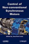
Many papers and books (most in French) since the beginning of the 1990s have developed the causal ordering graph (COG) formalism [BAR 04, HAU 99a]. It has been a very efficient graphical formalism for establishing physical models by representing causal relations and for designing control structures by using a principle of systematic inversion. Figure 7.5 presents the two main processors of the COG formalism: the accumulative and the dissipative processors, respectively.

Simple observation of the linear motor helps us to understand the causality of the energy transformation. Indeed, it appears that supplying the power cable with an adapted voltage will make the linear motor move to the desired position. This short analysis can be performed by applying the same principle using a graphical representation, here the COG, as depicted in Figure 7.6. We can see that the system inputs are the voltages of the primary (Vd, Vq) and the output is position x of the mover.

The PMLSM model in the first harmonic model can be represented in the Park reference frame in order to design vector control (including a self-control strategy).

This graphical representation offers the advantage of visually outlining the energy path, also called the “causal path”. For example, the voltages induce the currents, which generate the electromagnetic force (emf), which moves the motor at a certain speed. This representation helps us to understand the couplings between the flux and thrust axes of the model in the Park reference frame. Indeed, the thrust generated by the q-axis Tq can be modulated by the d-axis current id, allowing us to control the field weakening of the motor.

Finally, by using a visual approach, COG formalism facilitates the understanding and definition of physical models. We will see in the next section that the main advantage of this formalism is to offer a systematical method for the control of structure design, using the COG inversion principle.

7.1.6. Advanced modeling of linear synchronous motors

As with rotating motors, linear synchronous motors have some geometrical specificities that induce nonlinear thrust generation:

– emfs mainly have wave harmonics of ranks 5 and 7 that are related to concentrated or distributed windings. The emfs generate ripple forces on the thrust throughout all operating ranges. They are more prominent, however, in high-speed modes;

– fast transient currents enable high acceleration of the linear motor but induce local saturation of the magnetic circuit and cause inductances to behave in a nonlinear manner;

– the cogging and the end of primary effects, related to the geometric ends of the iron sheets (effects that only occur in the case of linear motors), generate detent forces that are particularly perceptible at low speeds. The detent effects are particularly disturbing for positioning devices because they occur even when there is no current supply.

In fine, these three phenomena result in the presence of ripple forces on the thrust generated by the PMLSM, with different areas of dominance.

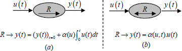
With the exception of end effects, all these phenomena exist in synchronous rotating machines and have been extensively modeled in the literature [GIE 03, REM 07]. Figures 7.8 and 7.9 give some examples of linear actuator geometry with end-effect compensation specific to linear motors. They show that the secondary ends may be optimized. Indeed, the main idea is to reduce the magnitude of the detent forces due to interaction between the magnets and the ferromagnetic teeth of the primary.

Figure 7.8 is from a patent [STO 98] that aims to cancel the fundamental of the cogging force, knowing that the periodicity of the phenomenon can be directly defined by the least common multiple between the period of magnet disposal and the period of tooth disposal.

Figure 7.10 shows the primary ends of the LMD10-050 designed by ETEL [WAV 97]. Here, the principle is that the cogging phenomenon can be divided into two parts: the extremities and the central part, as shown in Figure 7.11. Here, the central part is defined by the extremities as having periodic disposal of the ferromagnetic teeth. The compensation for the detent forces generated in the central part of a PMLSM is therefore equivalent to the compensation of a rotating motor’s detent forces, because it is a periodic area. The choice of the ratio between the tooth and the magnet width is then the way to reduce such cogging forces.

The idea is to cancel the ripple forces generated by the end-effects, and therefore to cancel several harmonics. The result obtained is shown in Figure 7.11. The waveform of the detent force is thus greatly reduced in amplitude (less than 4 N for the peak value) for an engine with a peak value of about 580 N. If we compare this with a more conventional geometry, this would have represented approximately 20 N in peak value.

It is important to note that a rigorous scientific decomposition of the phenomena resulting from the central part and the end-effects is only valid in a linear regime, and not in a saturated case. In the saturated case, when operating at the maximum current of the actuator, we have found a relatively small difference to the linear case results of around a few percentage points.

These phenomena are dependent on the level of actuator saturation and on magnet position, which impact locally on the level of saturation. Some results can be obtained using only a finite element analysis [REM 07] or reluctance network modeling [GOM 08].

These phenomena are only noticeable at low speeds, however, because the moving mass of the primary acts as a first-order filter between the ripple force and the motor speed. The objective of this chapter is not to focus on the advanced modeling of linear actuators alone. Interested readers can find therefore, more details about PMLSM modeling in [GIE 99] and [BOL 01].

7.2. Classical control of linear motors

7.2.1. State-of-the-art in linear motor controls

Nowadays, there are many strategies that can be used to control the thrust generation of a PMLSM [GIE 99]:

– Scalar controls regulating the amplitude of the signal to be controlled. This technique is mainly used in open-loop, as well as closed-loop, speed control for keeping the U/f ratio constant. This technique does not give satisfactory results for rotating motors in dynamic motion control. It is mainly used in applications such as roller coasters, where a very high positioning accuracy is not essential.

– Vector controls regulating the amplitude and phase vectors of the signal to be controlled. The control structure is usually placed in a reference frame linked to the secondary to perform decoupling of the flux and thrust of the motor. This technique is most widely used for controlling linear motors. To reduce the effects specific to linear motors (end effects, etc.), digital filters are inserted into the control structure in reality.

Both of these techniques currently use control structures with fixed and constant parameters. When the performances are no longer sufficient to control the system, however, the control structure becomes complicated:

– Auto-adaptive control or iterative learning control (ILC), which adjusts the variable parameters due to changes in the motor’s parameters. In applications such as “pick and place”, it is systematically used to increase the accuracy of repeatability.

– Sliding mode control, which switches between different control structures. The system is guided by a reference trajectory of successive commutations. The control is then insensitive to parameter and load variations. It is mainly used in applications such as magnetic levitation trains to differentiate between the control of starting and cruising phases.

– Control by neural network or fuzzy logic, where the mathematical model is not or is barely affordable by conventional identification. This has so far mainly been used in academic research.

The main difference between linear motor and rotating motor models is related to the fact that there are more harmonics with cogging forces (associated with the secondary ends) in a linear than a rotating motor. The conventional controls for rotating motors therefore cannot achieve maximum actuator performance. Indeed, the ripples of cogging force induce an imprecise thrust force control, which is insufficient in some cases (e.g. force feedback in the stick of a flight simulator) [REM 07].

The position sensor, however, is a much more sensitive component in linear actuators: it consists of a reading head on the primary and a graduated ruler that is deposited along the secondary (sometimes over several meters) and is therefore highly sensitive to its external environment. It is therefore able to detect mechanical deformations in torsion and/or bending, resulting from mechanical stress (high acceleration mode resonance, etc.) and thermal stresses. For applications calling for positioning accuracy of around the micrometer level, these distortions are particularly detrimental and lead to measurement errors, even measurement malfunction when the reading head moves away from the graduated ruler for more than 0.1 mm.

By expanding our research to industrial the control structures of synchronous machines, it appears that “nested loop” controls are the most widely used [GRO 01]. They mainly include controllers with proportional and integral (PI) or proportional, integral and derivative (PID) actions. They are easy to implement and tuning principles are now widely known in the industry. To satisfy the latest specifications that have become increasingly constraining, many applications now require more sophisticated control structures. So, two structures are currently competing:

– Control is obtained from a model of behavior (also called the black-box model), which is often characterized by controllers of a very high order (e.g. H∞ robust control). The difficulty with this kind of control is the order of model reduction. For the control structure to be able to operate in real time, the system transfer function has to be reduced from a high to a reasonable order. A high level of expertise is needed to accomplish these adjustments.

– Control is obtained from a model of knowledge that is deduced from the inversion of a model defined by the physical properties of the system’s components. To be highly effective, this kind of control structure requires a physical model that is as close as possible to reality. The synthesis of the control structure is then facilitated by the use of graphical formalism, such as the Bond-Graph [DAU 99], the COG [HAU 98] or the energetic macroscopic representation [BOU 00].

In the next section, to optimize the thrust generation of a linear motor, different control architectures are studied using the inversion principles of the COG. First, from the first harmonic model of a linear motor, we compare different types of closed-loop controls. Then, using the models presented in the preceding sections, we establish some control structures using different control techniques, especially on the electrical and magnetic phenomena that generate disturbing ripples on the thrust. In particular, we specify the tuning techniques for each control strategy, and then present the advantages and limitations of these different commands.

Finally, we present several open-loop control strategies and focus on the problems associated with generation of the reference variable in the case of a command using the nth derivative of the reference variable.

7.2.2. Control structure design using the COG inversion principles

Since the 1990s, COG formalism has been developed to facilitate the modeling and control design of systems based on understanding energy exchanges, and particularly the principle of causality. This vision arises naturally in control design, as “since we know the cause, it is sufficient to apply the right cause to obtain the right effect” [HAU 99a]. Thus, regardless of the control structure type (continuous, discrete, sampled, etc.), we seek an implicit inverse model of the process that is to be driven.

The control structure design using the formalism of the COG is based on the following concepts:

The organization of the control structure is deduced systematically from an inversion principle of the graphical representation of the system model. We can usually find direct processors that represent dissipative phenomena and causal processors, which are time-dependent and represent the accumulation phenomena in the process. It is therefore natural for the inversions of both processor types to obey different laws, as shown in Figure 7.13a.

On one hand, it is possible to reverse a direct processor as:

[7.3] 

where C is a time-independent function that represents the inverse of the surjective or bijective time-independent function R.

On the other hand, the inversion of a causal processor requires an indirect inversion (feedback control), as shown in Figure 7.13b.

[7.4] 

where C is the corrective function chosen according to the specifications of the desired system performance in closed loop. It can be demonstrated that for an indirect inversion, a proportional correction with high gain is sufficient to ensure convergence between the reference and the measurement of a linear time invariant system with non-minimum phase. Nevertheless, the controller choice is not defined by the COG inversion principle. Only control engineers can decide whether it is a proportional controller (P), an integral-proportional controller (IP) or a resonant controller, etc.

7.2.3. Closed-loop control

The indirect inversion principle of the COG is thus applied to the PMLSM model presented in Figure 7.6. Figure 7.14 shows a scheme of the control structure representation, also called maximum structure of control3 .

This type of control architecture is commonly called “cascaded closed-loop control”. Indeed, Figure 7.14 shows the indirect inversion principle of the COG applied to causal processors of the (R3d, R3q, R9, R11) model. This structure requires currents, speed and position sensors to be available. Three concentric loops are thus formed. A maximum control structure is therefore established very quickly, “processor after processor”.

Then, the Rc3d and Rc3q processors are inside the inner current loop, and both contain a PI controller. The Rc9 processor is inside the speed loop and contains a P controller, and the Rc11 processor is inside the outer position loop and contains a P controller. Figure 7.14 outlines the graphical simplicity of the COG representation that helps us to identify the energy links, successive energetic conversions and processors inside the cascaded closed-loop control.

Figure 7.15 shows us that the processors constituting the direct energy chain (Rc2d, Rc2q, Rc3d, Rc3q, Rc5d, Rc5q, Rc8, Rc9, Rc11) are involved in energy conversion. The presence of these processors is required to generate the manipulated variable from the reference variable. A perfect system in terms of energy means there is no dissipative loss; it could be controlled by a control structure without an estimation processor or the observers normally used to compensate for energy losses due to the effects of resistance or friction.

All hatched processors in the control structure contribute to the compensation of the imperfections of the process (for example, the resistive voltage drop of the resistance or friction force in the system). Indeed, Ro4d and Ro4q processors estimate the voltage drop of the resistance, such as:

[7.5] 

When the processor input comes from the measurement of a variable, as for the estimation or observation processors, they are represented by a hatched oval in Figure 7.14. The other control processors are grey on a white background. Thus, at a glance, the COG representation directly shows the role and impact of different variables on the control strategy.

7.3.3.1. Analysis of the current in a closed loop

Using the COG’s inversion principles, it is possible to define three types of current control architecture, as depicted in Figure 7.15. For ease of reading, we have chosen to show only the COG representation of the q-axis (also called the thrust axis).

The following assumptions are used:

– Vq = Vqreg, where the inverter is assumed to be ideal without delay;

– eq = eqest, and more broadly Vqreg − eqest = Vq − eq, the compensation for the emfs is assumed to be perfect in the speed loop;

– iqmes = iq, the initial angular value required to correctly achieve the Park transformation is assumed to be perfectly known, otherwise the value of iq is decomposed on the two axes idmes and iqmes. The measures are taken without delay and no measurement noise is considered.

The control architecture shown in Figure 7.15a comes directly from the COG inversion principle: a processor in the control structure to each processor of the model corresponds. All these processors are represented using a white background.

To compensate for the resistive voltage drop Vrq, the R4q processor is added to the control structure of Figure 7.15a and Figure 7.15b:

– in case a, the VRq value is deduced from the reference variable iqref,fi hence the name is VRqref. It is equivalent to a feed-forward control. However, if there is an error between the reference and the actual currents, then this error is amplified by the resistance value;

– in case b, we can use the current measurement to estimate the ohmic voltage drop. Thus, the objective is for the model to be as close as possible to reality. It is therefore an estimation of the reference voltage, VRqest. It follows that the processor is shaded and is called Ro4q;

– in case c, if we focus on the case of a steady-state current that corresponds to iqRef = cst, the ohmic voltage drop is constant and generates a constant error on current iq. Thus, in steady-state current, the static error can be compensated for by an integral action associated within the proportional controller in the Rc3q processor. In the end, if the estimation of the ohmic voltage drop is neglected (Ro4q and Ro4d processors) an integral controller must be added to the proportional one.

For the three cases studied, the relations (R2q, R3q, R4q) representing the process are equivalent:

[7.6] 

For the three structures depicted in Figure 7.14, the respective relations are written:

[7.7] 

The transfer functions in the closed loop of the three current loops are then expressed as:

[7.8] 

The Ci and C′i, controllers correspond to a P and a PI controller respectively:

[7.9] 

The choice of the PI controller aims to compensate for the electrical time constant of the actuator:

[7.10] 

ASSUMPTION 7.1.– the identification of Rq and Lq is perfect, and the expression in the case of PI controllers can be simplified:

[7.11] 

Thus, with ideal identification of the resistance and inductance parameters, the three transfer functions have no static error. Nevertheless, the three cases show different time constants, in each case depending on controller coefficients. The proportional gains of cases a and b have almost the same role: in case a: Ci = Ki − Rqest; while in case b, Ci = Ki. To ensure stability, Ci is positive (which means that Ki > Rqest). The main value of such a current controller is to improve system performance and especially the time response of the current loop. To reduce its time constant, it leads to Ki = K′i > Rq in equation [7.11] in cases b and c. In case a, if the ohmic voltage is known using a feed-forward control, the required gain value Ki for the controller will be lower than in other cases that are not anticipated. Here, the advantage of reducing the impact of the noise measured in the control is obvious.

In practice, determination of the controller coefficients has to be adapted to the physical limitations of the system. Here, the DC bus voltage Us modulated through the inverter limits the voltage of the linear motor. Thus, the maximum voltage available is Us. The dynamics and the bandwidth of the closed-loop current are thereby limited by the inverter’s maximum voltage. Whatever the type of control (cases a, b or c), the controller cannot solicit more of the inverter output voltage that the Us value. Consequently, using a proportional controller, for example, there are maximum gain values to prevent the inverter being saturated at -Us. and +Us and so to keep a linear control of the linear actuator. High gain values will lead to saturation of the inverter and so to nonlinear control: a so-called “bang-bang” control strategy. Even if this control strategy gives the fastest possible acceleration of the linear motor, it generally produces a large error between the thrust generated and its reference, and produces a large range of harmonics on the thrust, which engenders unacceptable vibrations of the yoke. The determination of the gain, Ki, could be done by calculating the maximum current error and by fully scaling the inverter. Then, the maximum current error will directly correspond to the maximum response voltage on the inverter.

7.3.3.2. Application to the linear motor studied (see Appendix, section 7.8)

In case a in Figure 7.15, Ki <= Us/errmax. iq, the maximum current error for a current step corresponds to the maximum current value. For the PMLSM studied, the DC bus voltage is limited to 300 V, so: Ki = 300 V/7.9 A = 36.97 Ω.

In case b, Ki <= 36.97 + Rqest = 41.37 Ω: the ohmic voltage drop is not anticipated.

In case c, Ki <= 41.37 Ω.

Figure 7.16 shows the three cases with the optimized gain to avoid inverter saturation. Response times are exactly the same and the limiting factor also remains the same in all three cases: i.e., DC bus voltage Us.

The closed-loop bandwidth is identical in all three cases. For this linear motor, the constant Lq/Rq is about 4.9 ms. The time response in closed loop is about 0.52 ms and the current bandwidth is about 300 Hz.

7.3.3.3. Influence of parameter variations

In the Ro4q processor, for an estimation error of Rq resistance, such as Rqest = . Rq, we get the following transfer functions:

[7.12] 

For case c, the integral action of the PI controller compensates for the error of the estimated resistance value: the static error tends to 0. For cases a and b using P controllers, however, there is a static error dependent on the estimation error of the ohmic voltage drop:

[7.13] 

7.3.3.4. Application to the linear motor studied (see Appendix, section 7.8)

Figure 7.17 shows that cases a and b give a static error on current iq, while the command with a PI controller converges to the correct value.

Figure 7.16b shows the response to a 20% estimation error of inductance Lq. The response in case c is affected by the estimation error: there is an overshoot of the reference but it finally converges with the reference value. Cases a and b are unaffected.

Unsurprisingly, the PI controller used makes the measured current converge to its reference value. The reasoning of the d-axis and that of the q-axis are the same because the two axes have similar behaviors. For linear motors with surface-mounted permanent magnets, however, the control architecture can be simplified by neglecting the d-axis component. Indeed, for such linear motors, and knowing that Lq = Ld, the expression of the thrust force was dependent on the current of the q-axis iq only. So, theoretically, current id does not influence the motion control of the linear motor. The feedback control on the d-axis current is therefore useful for performing a defluxing strategy or reducing the Joule losses. In this last case, current id is controlled to idref = 0.

7.3. Advanced control of linear motors

In the previous sections we have detailed how the controls of rotating motors can be applied to linear motors using the first harmonic model. Generally, the use of proportional and integral controllers is sufficient to assure speed control of linear motors. However, PI controllers appear to be insufficient due to the ripple force generated by the cogging force and end-effect force effects that only exists in linear motors.

Thus, using more sophisticated models, new control techniques are needed to take into account the specificities of linear motors:

– use of an auto-adaptive resonant controller to compensate for cogging forces;

– adding a feed-forward action in PI controllers in order to compensate for the detent forces. For example, it is possible to map the detent forces and to fill a lookup table. This could then be used in feed-forward anticipation as an added compensation of the detent forces;

‒ another solution would be to have a very detailed model and to deduce a more appropriate control strategy.

These are presented in the following sections.

7.3.1. Multiple resonant controllers in a two-phase reference frame

The principle of the resonant controller emerges from the need to eliminate the frequency error induced by the existing current and voltage harmonics [HAU 99b]. The equations of the resonant controller in the case of a sinusoid Csin [SAT 98] and a co-sinusoid Ccos [FUK 01] are defined by:

[7.14] 

To simultaneously control the amplitude and phase of a sinusoidal signal, a solution is deduced from the previous two equations [WUL 00]:

[7.15] 

This resonant controller is now used in many areas:

– control of active filters to limit electrical pollution in grids [GUI 00];

– control of power converters for high-frequency variation of the grids [GUI 07];

– optimization of the torque control of a synchronous machine [ZEN 04].

For the variable speed drive of linear motors, the frequency of reference currents is greatly variable. Thus, the resonant controller is called self-adaptive or auto-adaptive. The reference pulse p of the controller needs to be adapted to the desired or measured pulse at all times, as = p. The numerator coefficients of equation [7.15] are also defined at all times to ensure stability and high-level controller gains.

Figure 7.18 shows the command structure of the thrust force in the steady two-phase reference frame (, ) using resonant correctors.

Figure 7.19 shows the Bode diagrams of two-frequency series resonant controllers in open loop (BO) and closed loop (BF), in amplitude and phase. The first controller is set to operate at pulse p and the second at pulse p5.

Some of the properties of resonant correction are:

– at the pulse p, this transfer function has a module tending to an infinitely large value (about 300 dB, see Figure 7.19a). The gain is higher at the desired pulse and not across the frequency bandwidth. Thus, for a given stability criterion, the gain in value can be higher for the resonant controller than it can be for a PI controller. The convergence between the reference and the measurement is then faster than a conventional solution;

– the value of the gain being high at the pulse p, if the conditions of stability are guaranteed the frequency error will remain low, even for parameter estimation errors. This allows the resonant controller to be efficient;

– reducing the frequency error at the reference frequency causes the output variable to be in phase with the input reference variable, as shown in the closed-loop phase of the Bode diagram, in Figure 7.19b.

The two-phase reference frame is determined using the Concordia and inverse Concordia transformations, which are defined by the equations [LOU 04]:

[7.16] 

The transformation is only useful because the linear motor studied has a star connection and is balanced. This means that out of the three phases to be supplied, there are only two independent variables. Hence, a mathematical representation, or rather a reference frame, is needed where two parameters, called and , will be sufficient to independently control the currents.

Finally, two current references are generated to compensate for the influence of the emf on the thrust force:

[7.17] 

A resonant controller is then applied to two frequencies:

– on the fundamental of the emf to control the thrust force;

– on the rank 5 harmonic of the emf, using coefficient. 5 to eliminate the ripple force of the thrust generated.

There are many techniques to generate these reference variables. For one reference force, two reference currents must be generated, with as many frequency references as the number of frequencies to be controlled in the resonant controllers. There are therefore several degrees of freedom in the generation of reference currents.

Furthermore, the resonant controller is not directly applied to an error between the reference and the measurement of the emf. It is very difficult to determine the emf during motion without unplugging the power supply. Thus, the resonant controller is used on the current error only, and the harmonics of emfs are defined with a reference current generator, using the equations described in equation [7.17].

The work of [ZEN 05] specifies the tuning principle of a multiple resonant controller, and applies it to a multiple auto-adaptive resonant controller.

The tuning technique for each step of calculation is defined as follows:

– to evaluate the fundamental value of the reference pulse p, from the measured speed: p = . ν/τp;

– to control the harmonics of ranks 1 and 5. Then, the denominator coefficients are known:

so the characteristic polynomial of the closed-loop current is then expressed:

[7.18] 

– the numerator coefficients are calculated using a pole placement technique known as the “symmetrical optimum”, which guarantees the same time response for each harmonic [LOR 97, SHI 78].

so, the characteristic polynomial is simplified as follows:

[7.19] 

– limits for the resonant controller are fixed in terms of bandwidth and maximum phase;

– finally, the characteristic polynomial is solved using Gaussian elimination on the coefficient matrix for coefficients bn [ZEN 05].

In the case of the motor studied here, the resonant controller must compensate for 1.6% of the rank 5 harmonic of the emf [REM 07].

Experimental tests have been conducted in order to apply this resonant controller strategy to LSP120C, a linear motor created by Indramat, which has a two-phase reference frame (, ). Figure 7.21 shows that the results are satisfactory and that the estimated force completely follows the reference force [ZEN 04]. Furthermore, the zoom of Figure 7.21 reveals that the time response of the resonant controller is about 5 ms during fast acceleration. Furthermore, the real-time implementation of a multiple resonant controller with variable frequency can be achieved in a computation time less than the time step of feedback control: 26 µs of time calculation4 on the 50 µs admissible for the current loop, as can generally be found in industrial drives [GRO 01].

The results in Figure 7.22 show that the resonant controller allows the motor current to follow the reference current perfectly:

We have proved the use of the resonant controller technique in controlling linear motors.

An auto-adaptive resonant corrector is nothing more than a highly selective filter, with self-adaptive properties at given frequencies (see Figure 7.19). Equation [7.15] shows that the expression of the resonant controller is very close to that of the lead controller. However, it is the peak width in Figure 7.19 that guarantees the immunity of control from parasitic frequencies. So, if the value of the estimated frequency reference is not perfectly identified, a peak that is too fine will induce a greater risk of stalling the frequency tracking of the resonant controller.

Thus, the resonant controller can be a “miraculous” solution only if the resolution of the speed sensor is sufficient. Similarly, to control high-order harmonics, the speed error will be proportional to the harmonic rank and the risk of divergence will increase proportionately. To our current knowledge, there is no study showing the limits of the resonant controller, and this is beyond the scope of this book.

7.3.2. Feed-forward controlfor the compensation of detent forces

The principle of feed-forward control is to replace the estimation and observation processors using measurements of quantities (e.g. position, velocity and currents) with reference values given by reference variables and derivatives. Figure 7.23 shows a feed-forward control structure.

The feed-forward control is widely used in fields such as machine tools with linear motors [GRO 01]. In practice, this control structure allows us to keep a cascaded closed-loop control and add feed-forward compensation to each loop entry. The main idea is to reduce delays from one loop to the next. Yet, such compensation can only be effective if the system runs exactly as anticipated by the reference. Thus, although faster and more precise, this control structure is less resilient to unforeseen external forces.

It is rarely necessary to anticipate the current loop using PI controllers, however, as it is sufficiently fast and accurate, as shown in Figure 7.23. Indeed, although there are some disturbances in the motor current (e.g. from the pulse-width modulation – PWM) and because the current error remains low in amplitude, it generally leads to the improvements of this kind of control not being discerned on the current loop performances. Nevertheless, on the closed loop speed control for linear motors, the improvement can be very significant [GRO 01].

7.3.3. Commands by the nth derivative for sensorless control

The inversion principle of the control structure by the nth derivative is defined in the COG formalism as a direct inversion [BAR 04]. Figure 7.24 shows the direct inversion of rigid and causal processors:

Figure 7.24b shows that the inversion of a causal processor does not require measurement of the controlled variable, so no sensor is required here. Control by the nth derivative is based on the following principle: if a linear time invariant with minimum phase is a n-order system between an input control u and output variable y, then the evolution of this system can be established from the nth derivative of y:

[7.20] 

where ai and bi are constant coefficients. In all cases m < n, which ensures compliance with natural causality. The relationship expressed in the Laplace domain takes the form of the following transfer function:

[7.21] 

Control by the nth derivative derived in open loop is written:

[7.22] 

The assumption hidden in equation [7.22] is an important concept of control by the nth derivative: in fact, the performance of this control is based solely on the quality of the identification of the system’s parameter. This control structure is also known as early control [BEA 04]. It is important to note that three variables are essential to the PMLSM control in open loop:

– the input variables (here, the voltage supply);

– the controlled variables (here, the position of the linear motor); and

– the nth derivative of the controlled variable. This means the variable that defines all other variables in the system from a defined initial state (here, the third derivative of the position, i.e. the jerk).

Thus, this technique is applied to the PMLSM, with the position of the linear motor x as the output variable, and Vq as an input voltage of q-axis. First, the canonical representation of the first harmonic model of a linear motor is used in the Park reference frame:

[7.23] 

Figure 7.25 shows a COG representation of an open-loop control structure using the first harmonic model in the Park reference frame.

Here, in order to control the linear motor, it is necessary to define the inductance voltage VLq for a given displacement. This can be obtained by adapting equation [7.23] to a canonical equation that links acceleration and jerk:

[7.24] 

To control the position x of the linear motor, first we need to have defined the third derivative of the position, i.e. the jerk. Then, from this variable and all the initial values of the state variables, all of the states of the system can be calculated, which means that we can find the acceleration, velocity and position at any time. Finally, using the inductance voltage is enough to rebuild all the system states starting from an initial state.

Although the control in Figure 7.25 involves a large number of processors, reading is very intuitive as it allows us to recreate the set of states of the system.

This control architecture is simulated in the case of the motor studied, for a displacement of 0.2 m at 2 m/s and 20 m/s2, using a jerk bang-bang. The following results are obtained:

Figure 7.26a shows the simulation of the nth derivative control technique in the case of PMLSM using the first harmonic model. The results show that such a technique is efficient. Figure 7.26b shows the application of this technique in a more realistic way, because it includes the emf harmonics, the inductance saturation effects and the detent force. Furthermore, it shows that the results deviate slightly from those in Figure 7.26a, where an error of 4 mm in position can be seen at the end of a 260 mm displacement (with 1.5% as the maximum position error). Moreover, the speed has an error of about 0.05 m/s, regarding the 2 m/s desired (with 2.5% as the maximum speed error). Finally, for the thrust generated, the maximum error is 4 N, regarding the 20 N desired, for a 20% error. Although there is no external disturbance, the force control is not precise enough.

Thus, it is necessary to extend the force control to the q-axis using the full first harmonic model of the linear motor. This means no longer neglecting the influence of the d-axis, including the emf ed.

If we analyze the control structure in Figure 7.25 more precisely, between the input and the output variables, the direct chain has three causal processors (Rc11, Rc9 and Rc3q), and the nth derivative of this system is a third-order system. In the representation in Figure 7.25, the variables corresponding to the third-order derivative are the inductance voltages VLd and VLq of axes d and q, respectively. This means that the inductance voltages must mathematically be of at least class C3 to respect the continuity of the whole system.

Thus, with a very accurate model of the system and being able to generate the nth derivative of position x, it is possible to obtain absolute control of the linear motor. Figure 7.25 shows that this kind of control does not use any current sensor.

When using this control technique, it is important to highlight the weak points.

If the friction and detent forces are not neglected, generation of the reference variable is much more complicated. In fact, it becomes necessary to know the derivative of the friction and the detent forces, which are highly nonlinear, in order to generate the derivative of the reference acceleration:

[7.25] 

So even if the third derivative of the reference position is known, it is difficult to directly define the inductance voltage reference. This reference is not causal and therefore generates significant discontinuities in the force reference, mainly at each speed inversion on the friction force.

Figure 7.27 compares the reference, measurement and simulation results to a bang-bang jerk profile with 20 m/s2, at 2 m/s for a 20 cm displacement.

The open-loop control uses the strict inversion of the model. It is therefore the ideal control structure, since it allows us to entirely anticipate the behavior of the system. Nevertheless, the generation of the reference variable (nth derivative) in the open-loop control is the major problem with this kind of control. The physical limits of the linear motor must be taken into account in the generation of reference variables, since there are no sensors to protect the engine.

Obviously, the generation of the reference variable is the main problem in the case of our nonlinear model of a linear motor. The flatness control appears to be a possible alternative for controlling the linear motor in open loop [FLI 92]. This approach may be coupled to learning methods by successive iteration (known as iterative learning).

7.4. Conclusion

It is clear that linear motors have undeniable advantages for rapid implementation in industrial applications: increasingly, systems are using direct drive (they are cheaper, have fewer components in the transmission, etc.). Initially, the formalism of the COG allows us to find the same control structures as industrial structures using the first harmonic model of the actuator. Obtaining very high performances from such actuators requires the definition of a highly detailed physical model of the linear motor concerned.

This chapter has shown the inherent specificities of linear motors and their impact on thrust generation. In particular, the generation of force ripple can be controlled by the control design using resonant controllers, which can dynamically compensate for multiple parasitic harmonics or frequencies. Another approach that has been discussed in this chapter is the open-loop control of linear motors using a direct inversion of the COG representation. Such a sensorless control strategy could be very efficient in friction-free linear motors equipped with very high-speed inspection machines and used in the semiconductor industry. However, the drawback with this model is that the open-loop control is very sensitive to modeling errors and to variations in parameter.

Finally, knowing how to graphically design the control structure of an actuator enables us to obtain the adapted performance of the system. The next step is to redesign the geometry of the motor itself: Even if the efficiency of the motor might be reduced, the main idea is to improve the whole system performance. An example of this mechatronic approach could be to geometrically design a linear motor with a perfect sinusoidal cogging force instead of trying to reduce the force to low amplitude. Even if the cogging forces are greater in amplitude, it may be easier to have a sinusoidal waveform to compensate for cogging forces in the control design. And so, better performances for system positioning will be achieved and the vibration of the mechanical yoke could be reduced.

7.5. Nomenclature

	Estimated or calculated X variable,
	MeasuredX variable
	Maximum value of the X variable
Vd, Vq	Voltage of the d-axis and the q-axis, in Park reference frame [V]
Vdref, Vqref	Voltage references of Vd, Vq, in Park reference frame [V]
ed, eq	Electromotive forces ed of the d-axis and eq of the q-axis, in Park reference frame [V]
,	Estimations of ed, eq, in Park reference frame [V]
id, iq	Currents of the d-axis and q-axis, in Park reference frame [A]
idref, iqref	Reference current id and iq, in Park reference frame [A]
kd, kq	Electrical factors of d-axis and q-axis, in Park reference frame [N/A]
	Estimations of kd and kq, in Park reference frame [N/A]
Ld, Lq	Inductances Ld of d-axis and Lq of q-axis, in Park reference frame [H]
	Estimations of Ld, Lq, in Park reference frame [H]
L	Inductance of one phase of the primary of the PMLSM, in the abc reference frame [H]
R	Resistance of one phase of the primary of the PMLSM, in the abc reference frame [Ω]
M	Mass of the primary of the PMLSM [kg]
Tem, Temref	Thrust force and reference of thrust force [N]
Tr	Load force [N]
	Pole pitch — the distance between two consecutive magnetic poles — for the PMLSM [m]
Np	Electrical constant of position: Np = /τp [rad/m], for a rotating motor: Np = p, with p being the number of pole pairs
x	Linear displacement [m]
	Mechanical angle of the rotor for a rotating motor [rad]
	Electrical angle [rad]
	Maximum value of the magnetic flux of induction for each phase in the abc reference frame [Wb]
ν	Linear speed [m/s]
Ω	Mechanical angular speed for a rotating motor [rad/s]
	Electrical angular speed or electrical pulsation [rad/s]

7.6. Acknowledgment

This work has been supported by ETEL’s Research Team, including Ralph Coleman, Motion Control Research Manager, and his team working on the control of linear actuators and collaborating with the L2EP (Department of Electrical Engineering and Power Electronics of Lille, France).

7.7. Bibliography

[ANO 04] ANORAD, “Precision gantry systems, (HPG) high precision gantries, (SPG) super precision gantries, (UPG) ultra precision gantries”, Catalogue Anorad, 2004. (Available at: http://www.rockwellautomation.com/anorad/index.html, accessed December 2008.)

[BAR 98] BARRE P.J., CARON J.P., HAUTIER J.P., LEGRAND M., Systèmes Automatiques, Tome 1 Analyses et modèles, Ellipses Marketing, 1998.

[BAR 04] BARRE P.J., Commande et entraînement des machines-outils à dynamique élevée – formalismes et applications, thesis, USTL de Lille, France, December 2004.

[BOL 85] BOLDEA I., NASAR S.A., Linear Motion Electromagnetic Systems, Wiley Publishing, New York, 1985.

[BOL 97] BOLDEA I., NASAR S.A., Linear Electric Actuators and Generators, Cambridge University Press, Cambridge, 1997.

[BOL 01] BOLDEA I., NASAR S.A., Linear Motion Electromagnetic Devices, Taylor & Francis, London, 2001.

[BOU 00] BOUSCAYROL A., DAVAT B., DE FORNEL B., FRANÇOIS B., HAUTIER J.P., MEIBODY-TABAR F., PIETRZAK-DAVID M., “Multimachine multiconverter system: application for electromechanical drives”, European Physics Journal - Applied Physics, vol. 10, no. 2, pp. 131-147, 2000.

[BRA 00] BRANDENBURG G., BRUCKL S., DORMANN J., HEINZL J., SSCHMIDT C., “Comparative investigation of rotary and linear motor feed drive systems for high precision machine tools”, Proceedings of the 6th International Workshop on Advanced Motion Control, pp. 384-389, April 2000.

[CAS 03] CASSAT A., CORSI N., WAVRE N., MOSER R., “Direct linear drives: Market and performance status”, LDIA2003, Proceedings of the 4th International Symposium on Linear Drives for Industry Applications, Birmingham, UK, September 8-10, 2003.

[CON 89] CONSTANT O., “L'Aérotrain, 15 ans après”, Voies Ferrées, no. 52, September-October 1989.

[COR 07] CORSI N., COLEMAN R., PIAGET D., “Status and new development of linear drives and subsystems”, LDIA2007, Proceedings of the 6th International Symposium on Linear Drives for Industrial Applications, Lille, France, 2007.

[DAU 99] DAUPHIN-TANGUY G., RAHMANI A., SUEUR C., “Bond graph aided design of controlled systems”, Simulation Practice and Theory, vol. 7, pp. 493-513, 1999.

[EAS 02] EASTHAM J.F., TENCONI A., PROFUMO F., GIANOLIO G., “Linear drive in industrial application: State of the art and open problems”, Proceedings of the International Conference on Electrical Machines (ICEM'02), CD-ROM, Bruges, Belgium, August 2002.

[ETE 07] ETEL, Linear Motors Handbook, ETEL, October 2007, (Available at: http://www.etel.ch, accessed December 2008.

[FAV 00] FAVRE E., BRUNNER C., PIAGET D., “Principes et applications des moteurs linéaires”, J’Automatise, no. 9, March-April 2000.

[FLI 92] FLIESS M., LEVINE J., MARTIN P., ROUCHON P., “Sur les systèmes non linéaires différentiellement plats”, Comptes Rendus des Séances de l'Académie des Sciences, vol. I-315, pp. 619-624, 1992.

[FUK 01] FUKUDA S., YODA T., “A novel current-tracking method for active filters based on a sinusoidal internal model”, IEEE Transactions on Industry Applications, vol. 37, no. 3, pp. 888-895, 2001.

[GIE 99] GIERAS J.F., PIECH Z.J., Linear Synchronous Motors: Transportation and Automation Systems, CRC Press, New York, 1999.

[GIE 03] GIERAS J.F., “Status of linear motors in the United States”, Proceedings of the 4th International Symposium on Linear Drives for Industry Applications, LDIA2003, Birmingham, UK, September 8-10, 2003.

[GOM 05] GOMILA G., Le Moteur Linéaire, sans Rival en Vitesse et Précision, Mesures, Paris, France, no. 774, 2005.

[GOM 08] GOMAND J., “Analyse de systèmes multi-actionneurs parallèles par une approche graphique causale - application à un processus électromécanique de positionnement rapide”, Electrical Engineering Thesis, Arts et Métiers Paristech (ENSAM) de Lille, France, 4 December 2008.

[GRO 01] GROß H., HAMANN J., WIEGARINER G., Electrical Feed Drives for Automation Technology - Basics, Computation, Dimensioning, VCH Publishers, Germany, 2001.

[GUI 00] GUILLAUD X., HAUTIER J.P., WULVERICK M., CRESPI F., “Multiresonant corrector for active filter”, Industry Applications Conference 2000. Conference Record of the 2000 IEEE, vol. 4, pp. 2151-2155, October 8-12, 2000.

[GUI 07] GUILLAUD X., DEGOBERT P., TEODORESCU R., “Use of resonant controller for grid-connected converters in case of large frequency fluctuations”, EPE2007, 12th European Conference on Power Electronics and Applications, Aalborg, Denmark, September 2007.

[HAU 98] HAUTIER J.P., CARON J.P., Systèmes Automatiques, Tome 2 Commande des Processus, Ellipses Marketing, Paris, France, 1998.

[HAU 99a] HAUTIER J.P., CARON J.P., Convertisseurs Statiques: Méthodologie Causale de Modélisation et de Commande, Editions Technip, Paris, France, 1999.

[HAU 99b] HAUTIER J.P., GUILLAUD X., VANDECASTEELE F., WULVERYCK M., “Contrôle de grandeurs alternatives par correcteur résonant”, Revue Internationale de Génie Électrique, vol. 2, pp. 163-183, 1999.

[LOR 97] LORON L., “Tuning of PID controllers by the non-symmetrical optimum method”, Journal Automatica (Journal of IFAC), vol. 33, no. 1, 1997.

[LOU 04] LOUIS J.P., Modèles pour la Commande des Actionneurs Électriques (Traité EGEM, Série Génie Électrique), Hermès-Lavoisier, Paris, 2004.

[MCL 88] MCLEAN G.W., “Review of recent progress in linear motors”, Electric Power Applications, IEE Proceedings B, vol. 6, pp. 380, 1988.

[NAS 76] NASAR S.A., BOLDEA I., Linear Motion Electric Machines, Wiley Publishing, New York, 1976.

[REM 07] REMY G., Commande optimisée d'un actionneur linéaire synchrone pour un axe de positionnement rapide, Electrical Engineering Thesis, Arts et Métiers Paristech (ENSAM) de Lille, France, December 12, 2007.

[SAT 98] SATO Y., ISHIZUKA T., NEZU K., KATAOKA T., “A new control strategy for voltage-type PWM rectifiers to realize zero steady-state control error in input current”, IEEE Transactions on Industry Applications, vol. 34, no. 3, pp. 480-486, 1998.

[SHI 78] SHINNERS S.M., Modern Control System Theory and Application, Addison-Wesley, Boston, USA, 1978.

[STO 98] STOIBER D., Synchronous Linear Motor, Krauss-Maffei AG, US Patent US005744879A, April 28, 1998.

[THY 08] THYSSENGRUP AG – TRANSRAPID, High-Tech for “Flying on the Ground”, Maglev System Transrapid, 2008 (Available at: http://www.thyssenkrupp.com/documents/transrapid/TRI_Flug_Hoehe_e_5_021.pdf, accessed December 2008.)

[WAV 97] WAVRE N., Permanent-Magnet Synchronous Motor, U.S. Patent 05642013A, June 24, 1997.

[WUL 00] WULVERYCK M., Contrôle de courants alternatifs par correcteur résonant multifréquentiel, Thesis, Université des Sciences et Technologies de Lille, France, June 2000.

[ZEH 02] ZEHDEN A., Elektrische Beförderungsanlage, Patent no. 26847, Charlottenburg, Germany, June 1902.

[ZEN 04] ZENG J., REMY G., DEGOBERT P., BARRE P.J., “Thrust control of the permanent magnet linear synchronous motor with multi-frequency resonant controllers”, Maglev 2004, 18th International Conference on Magnetically Levitated Systems and Linear Drives, vol. 2, pp. 886-896, Shanghai, China, December 2004.

[ZEN 05] ZENG J., High-Performance Control of the Permanent Magnet Synchronous Motor using Self-Tuning Multiple-Frequency Resonant Controllers, PhD Thesis, Lille University of Science and Technology, France, 21 September 2005.

---

1 Chapter written by Ghislain REMY and Pierre-Jean BARRE.

1 Linear motors are mainly known as direct drive, as opposed to rotary motors which are coupled with a mechanical conversion device, such as a belt-pulley, conveyor/timing belt, rack and pinion, lead screw, etc., which are termed linear axis.

2 To make reading easier, the anagram PMLSM will replace the following expression: “Permanent magnet linear synchronous motor with short primary, iron core and that is single sided”, as shown in Figure 7.4.

3 Note that it is only a maximum control structure for the model to be controlled. A more detailed model of the system would require us to redefine a new maximum control structure.

4 These results are obtained by taking into account the possibilities of the technology used: DS1005 dSPACE ® 400 MHz [ZEN 05].

7.8. Appendix: LMD10-050 Datasheet of ETEL