
Artificial Neural Networks for Predicting the Energy Behavior of a Building Category
A Powerful Tool for Cost-Optimal Analysis
F. Ascione1, N. Bianco1, R.F. De Masi2, C. De Stasio1, G.M. Mauro1 and G.P. Vanoli2, 1Università degli Studi di Napoli Federico II, Napoli, Italy, 2Università degli Studi del Sannio, Benevento, Italy
Abstract
The reliable assessment of building energy performance requires significant computational times. The chapter handles this issue by proposing an original methodology that employs artificial neural networks (ANNs) to predict the energy behavior of all buildings of an established category. The ANNs are generated in MATLAB by using EnergyPlus simulations for testing and training purposes. The inputs are properly set by means of a thorough preliminary sensitivity analysis. The final aim is a reliable assessment of the global cost for space conditioning as well as of the potential global cost savings produced by energy retrofit measures for each category’s building. The benefit is a huge reduction of computational times compared to standard reliable simulation tools. Definitely, this can support the diffusion of rigorous approaches for cost-optimal energy retrofits. Beyond the presentation of the methodology, this is applied to the office building stock of South Italy built in the period 1920–1970. The results show a high ANN reliability compared to EnergyPlus simulations, with regression coefficients (R) always higher than 0.98.
Keywords
Building dynamic simulation; energy retrofit; building category; global cost; cost-optimal analysis; surrogate models; artificial neural networks; sensitivity analysis; building sampling; office buildings
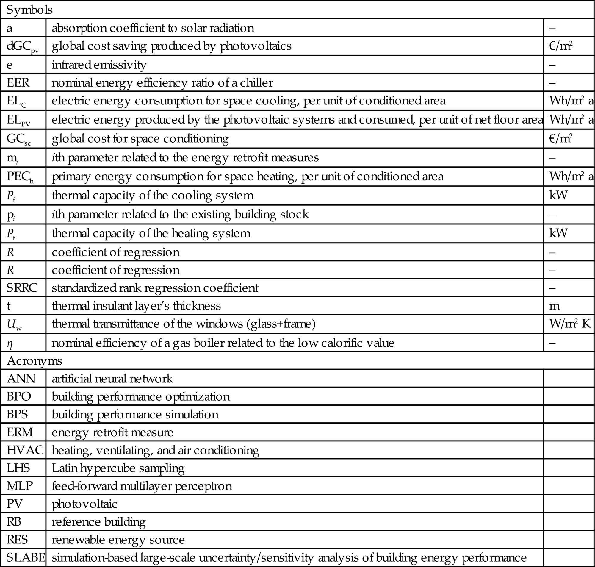
Nomenclature
| Symbols | ||
| a | absorption coefficient to solar radiation | – |
| dGCpv | global cost saving produced by photovoltaics | €/m2 |
| e | infrared emissivity | – |
| EER | nominal energy efficiency ratio of a chiller | – |
| ELC | electric energy consumption for space cooling, per unit of conditioned area | Wh/m2 a |
| ELPV | electric energy produced by the photovoltaic systems and consumed, per unit of net floor area | Wh/m2 a |
| GCsc | global cost for space conditioning | €/m2 |
| mi | ith parameter related to the energy retrofit measures | – |
| PECh | primary energy consumption for space heating, per unit of conditioned area | Wh/m2 a |
| Pf | thermal capacity of the cooling system | kW |
| pi | ith parameter related to the existing building stock | – |
| Pt | thermal capacity of the heating system | kW |
| R | coefficient of regression | – |
| R | coefficient of regression | – |
| SRRC | standardized rank regression coefficient | – |
| t | thermal insulant layer’s thickness | m |
| Uw | thermal transmittance of the windows (glass+frame) | W/m2 K |
| η | nominal efficiency of a gas boiler related to the low calorific value | – |
| Acronyms | ||
| ANN | artificial neural network | |
| BPO | building performance optimization | |
| BPS | building performance simulation | |
| ERM | energy retrofit measure | |
| HVAC | heating, ventilating, and air conditioning | |
| LHS | Latin hypercube sampling | |
| MLP | feed-forward multilayer perceptron | |
| PV | photovoltaic | |
| RB | reference building | |
| RES | renewable energy source | |
| SLABE | simulation-based large-scale uncertainty/sensitivity analysis of building energy performance | |
11.1 Introduction and Literature Review: Surrogate Models in Building Applications
One of the most important challenges of our generation is the change toward sustainable development in order to allow a low-carbon, green, and better future. We have the moral obligation to leave a clean environment, a proper lifestyle and new economic possibilities to our children. These are also some of the main aims and scopes of the “Roadmap for Moving to a Competitive Low-Carbon Economy in 2050” (EU COM 112/2011), which aims to pursue a 80–95% reduction in greenhouse emissions by 2050, compared to 1990 levels. To achieve this goal, first of all a substantial change is required for improving the energy performance of the building sector, since the activities related to buildings’ construction and management have a huge impact on global energy usage and related polluting emissions. This is true in the European Union (EU), where the buildings require about 40% (Odyssee, 2012) of the primary energy demand, as well as at the world level, with an impact around 32% being estimated (Khatib, 2012). Starting from this brief introduction, it is clear that all countries are engaged in an arduous political effort to establish new rules concerning building energy design. This has led to the standard of net and nearly zero-energy buildings (nZEBs), which will soon be mandatory for new constructions in order to reduce the energy requests of the future building stock. On the other hand, it is well known that the building stock, mainly in developed countries, is characterized by very low turnover rates, variable between 1% and 3% yearly. This implies that no significant outcomes will be achieved in the path toward a sustainable building sector if the existing stock is not subjected to a deep energy renovation (Caputo and Pasetti, 2015; Ma et al., 2012). In this framework, when a wide building stock is approached, the design of the energy retrofit gets extremely complex, as the buildings’ peculiarities are very different and various regarding the kind of envelope, the active energy systems, the possibility of integration from renewable energy sources (RESs), the building use, and the building value. Additional difficulties occur when the architecture is protected as Cultural Goods, which is very frequent in Europe, mainly in the Mediterranean area. Generally, there are two main actors involved. Indeed, from the point of view of the collective, the main target is an energy refurbishment aimed at achieving the highest reduction of energy usage and environmental impact. On the other hand, the private stakeholder (e.g., the building owner) also has to achieve an economic profitability derived from the energy retrofit. These aims very often are divergent, so that, in order to promote and realize effective refurbishments, the best tradeoff has to be found. This issue is considered by the Energy Performance of Buildings Directive (EPBD) recast (2010/31/EU) (EU Commission and Parliament, 2010), which introduces a new approach to energy efficiency by prescribing that the measures for building energy design or retrofit have to be chosen in order to achieve “cost-optimal levels.” The cost-optimal solution is identified by the lowest global cost, by taking into account the initial investment, the operating costs and the replacement costs, with reference to a conventional building lifespan, which is 30 years for dwellings and 20 years for non-residential buildings. More in detail, the step-by-step method for applying the methodology is defined in the EU Delegated Regulation No. 244/2012 (EU Commission, Commission Delegated Regulation (EU) No. 244/2012, 2012). Definitely, cost optimality is a powerful tool for ensuring benefits to all involved stakeholders, and thus economic convenience, technical feasibility, and environmental benefits for the community. All these concepts, benefits, implications, as well as a general description, are provided in (BPIE, 2013; Pikas et al., 2015). It should be noted that the main driver of the cost-optimal approach is economic feasibility; on the other hand, some other rigorous methods for a proper and effective building energy design are possible in order to achieve building performance optimization (BPO). The aim is addressing different objectives in order to explicitly satisfy particular interests and targets of the referred-to stakeholders. Generally, the goals of the involved actors are divergent, so that multiobjective optimization becomes the most suitable way to approach the design because it allows the simultaneous optimization of different objective functions. Commonly, among these, the targets to be achieved include minimizing the energy requests (Magnier and Haghighat, 2010; Diakaki et al., 2010; Chantrelle et al., 2011; Echenagucia et al., 2015; Ascione et al., 2015a, 2015b), the management and operating costs (Wright et al., 2002; Ascione et al., 2016), the initial expenditure (Diakaki et al., 2010; Chantrelle et al., 2011; Ascione et al., 2015a; Hamdy et al., 2011), the discomfort conditions (Magnier and Haghighat, 2010; Chantrelle et al., 2011; Ascione et al., 2015b, 2016), and the emission of greenhouse gases (Diakaki et al., 2010; Fesanghary et al., 2012). Furthermore, it is highlighted that cost-optimal analysis and multiobjective BPO are not mutually exclusive, but they can be coupled in order to have a more robust assessment of cost optimality. In other words, even if economic usefulness remains the main driver, other weights are given to further goals, such as the minimization of thermal discomfort or the reduction of initial expenditure (e.g., if the owners has a limited availability of investment) and polluting emissions (Hamdy et al., 2013; Ascione et al., 2015c).
Globally, with reference to each of the described robust methods for approaching energy retrofit design, the first step is the reliable prediction of building energy performance, concerning both the current configuration of the building and the explored retrofit scenarios. In that regard, all evaluation procedures and algorithms based on the resolution of the heat transfer through steady-state or semisteady-state calculation methods are inadequate. Indeed, these do not contemplate the transient heat transmission through the building envelope, and thus the effects due to rapid variability of forcing conditions (indoor and outdoor temperatures, instantaneous gains, solar radiation). Conversely, a proper choice is the adoption of building performance simulation (BPS) tools, which are capable of running transient (i.e., dynamic) energy simulations so that all tailored boundary conditions, starting from accurate hourly weather data files, can be implemented. The discussion concerning this topic is quite large in the available literature. In detail, Poel et al. (2007) reviewed the most used and popular methodologies and software for the building energy simulation. Several programs are today available, and the choice is not unique but, definitely, depends on computational time, level of accuracy, and quality of inputs (Richalet et al., 2001). Among them, the most frequently used are EnergyPlus (US Department of Energy, 2013), TRNSYS (Trnsys, 2000), ESP-r (ESP-r), and IDA ICE (IDA-ICE). These run transient simulations that ensure a reliable assessment of building energy requests, so that the impact of different energy retrofit measures (ERMs) can be accurately identified, thereby allowing robust feasibility studies. On the other hand, they imply high computational efforts, because of the complexity of transient (and thus reliable) energy simulations along the entire year with subhourly time steps. Moreover, a comprehensive design of energy refurbishments requires a huge number of energy simulations in order to investigate all possible scenarios, and therefore the computational issue dramatically intensifies. Of course, very often days or even weeks are unavailable for performing the energy investigations, so that alternative reliable procedures are required. This is probably the reason behind the choice carried out by the European technicians and legislators to define a set of reference buildings (RBs) (Corgnati et al., 2013) in order to represent the variability of the national stock. In this way, once cost-optimal packages of ERMs for the RBs have been identified, these would be successful for all buildings of the represented categories. However, how robust is the application of ERMs, calculated for a RB, to several heterogeneous buildings? Of course, there would be always a kind of indetermination, compared to an optimal energy retrofit solution dedicated (i.e., ad hoc) to the specific building under investigation (Mauro et al., 2015). Only in this way, all parameters – connected to building energy behavior, from the thermophysics to the wills and needs of occupants – can be taken into consideration. Definitely, if only a minimal uncertainness is accepted, energy evaluations must be performed for each specific building. Is it possible to do this with a satisfactory reliability and, at the same time, with suitable computational efforts and costs? A possible answer can be found in surrogate models (Kleijnen, 1987), also known as metamodels. This “model of the model” is built as a function of the design variables, able to emulate a more complex original one, based on computationally expensive computer models, by well approximating the objective functions. Surrogate models are defined starting from the data previously derived by performing several evaluations of the objective functions with the original model. Thus, the development of surrogate models is not immediate even if, once built, they are highly useful, being capable of fast and rigorous assessments. There are various techniques for metamodeling, among which the most used are multivariate adaptive regression splines (MARS), Kriging (KG), radial basis function (RBF), artificial neural networks (ANNs), and support vector regression (SVR). In order to have a general overview of methodologies and applications, the admirable study by Li et al. (2010) is recommended. Of course, for a successful metamodeling, the proper selection of the employed surrogate model is necessary, and this choice is related to the given problem that should be solved. KG, SVR, and ANNs are the most adopted techniques for the prediction of building energy performance, and several studies are already available including (Hopfe et al., 2012; Tresidder et al., 2012) for KG, (Dong et al., 2005; Brown et al., 2012; Eisenhower et al., 2012b) for SVR, and (Magnier and Haghighat, 2010; Kalogirou, 2000; Mihalakakou et al., 2002; Gonzalez and Zamarreno, 2005; Karatasou et al., 2006; Ekici and Aksoy, 2009; Popescu et al., 2009; Dombayci, 2010; Mena et al., 2014; Paudel et al., 2014; Kalogirou et al., 2001; Neto and Fiorelli, 2008; Kalogirou and Bojic, 2000; Asadi et al., 2014; Ferreira et al., 2012; Melo et al., 2014; Buratti et al., 2014) for ANNs. Notably, ANNs are the dominant surrogate models for building applications because they have a stable and satisfactory performance when the size of the domain is large (Li et al., 2010) and this is the case of the studies regarding buildings. Moreover, ANNs are preprogrammed in some authoritative software to solve mathematical and physical problems (Magnier and Haghighat, 2010), among which we would highlight MATLAB (MATLAB—MATrixLABoratory, 2010), as it is the one used here.
In detail, ANNs were applied in (Mihalakakou et al., 2002; Gonzalez and Zamarreno, 2005; Karatasou et al., 2006; Ekici and Aksoy, 2009; Popescu et al., 2009; Dombayci, 2010; Mena et al., 2014; Paudel et al., 2014) for predicting the hourly energy demand for the microclimatic control of buildings, as well as for evaluating heating and cooling loads (Kalogirou et al., 2001; Neto and Fiorelli, 2008), annual energy requests (Magnier and Haghighat, 2010; Kalogirou and Bojic, 2000; Asadi et al., 2014), and indoor conditions and achievable thermal comfort (Magnier and Haghighat, 2010; Asadi et al., 2014; Ferreira et al., 2012). Furthermore, ANNs were also used to investigate entire stocks (Melo et al., 2014; Buratti et al., 2014). We would like to mention that, with reference to the cited studies, the indices for evaluating the ANNs’ reliability were very favorable; in particular, the regression coefficient (R) in most cases was higher than 0.9. Actually, the generation of an accurate surrogate model aimed at evaluating the energy performance of buildings is a quite long process that requires many preliminary simulation studies by means of BPS simulations. This is the reason for which it makes poor sense to generate metamodels able to predict and perform energy studies only for single buildings, even if in some cases (e.g., for complex optimization studies that require an enormous number of energy simulations) it could also be useful to define a surrogate model for a specific building. However, the best use of surrogate models is when they provide predictions concerning entire building groups, so that the benefits that can be achieved, in terms of savings of computational efforts, are hugely evident and thoroughly exploited. Indeed, in this case, the computational time required for the development of the model itself is completely justified, as the model will be very usable for future studies. In fact, the same model can be used for predicting the energy performance of many and different buildings, even if they are in the same category, with required computational time highly reduced compared to the traditional approach of many single simulations by means of BPS tools.
This is one of the main motivations of this paper. More in detail, a new methodology based on the use of ANNs is proposed for a reliable and robust prediction of the global cost for space conditioning as well as of the potential global cost savings produced by ERMs. The model can be applied successfully to each member of a building category and two groups of ANNs are developed. These are generated by means of MATLAB by employing the outcomes of EnergyPlus simulations in order to test and train the networks. The first group of ANNs allows the assessment of energy performance of existing buildings (i.e., existing stock), while the second group addresses the prediction of potential global cost savings due to the implementation of ERMs. A preliminary study is performed to support the screening of the ERMs and to optimize the development of the ANNs. For this purpose, the SLABE methodology (simulation-based large-scale sensitivity/uncertainty analysis of building energy performance), proposed by Mauro et al. (2015), is employed. The investigated ERMs consider all levers affecting energy performance, namely the building thermal envelope, the energy systems, and the exploitation of RESs.
The main novelty of this study is the application of the ANNs for predicting not a generic but a specific response concerning energy performance and retrofit potential for any building of an established category. This innovative use of ANNs can offer a tool for enormously reducing the computational times required by a reliable assessment of building energy performance, pre- or postretrofit. Of course, this benefit is more and more significant if a proper energy retrofit design is carried out, thus the need to explore numerous scenarios. To that end, the proposed methodology can be a powerful tool for allowing and supporting the application of rigorous and reliable energy audits, as well as of effective, cost-optimal energy building retrofits.
In the next sections, the methodology is described and then applied to a real case study, namely the office building stock built in South Italy between 1920 and 1970 (i.e., the building category previously studied by Mauro et al. (2015) using SLABE). Therefore, the results achieved by Mauro et al. (2015) are used for selecting the ERMs and for optimizing the development of the ANNs.
11.2 Methodology: Predicting the Energy Behavior of a Building Category by ANNs
ANNs are used to predict energy performance and energy retrofit potentials for any member (i.e., building) of an established building category. In particular, different ANNs are developed in order to pursue two main goals:
GOAL I. Assessing the global cost required by space conditioning (GCsc) for any category’s member in its current configuration (as is)
GOAL II. Assessing the value of GCsc for any refurbished category’s member when energy retrofit measures (ERMs) are applied for the reduction of space-conditioning energy needs; furthermore, also the global cost savings (dGCpv) produced by the implementation of photovoltaic (PV) systems shall be predicted in conjunction with the other investigated ERMs.
Compared to standard BPS tools, the developed ANNs provide a good (i.e., slightly lower) reliability and a drastic reduction of computational times, as shown in the following paragraphs of this chapter. An ANN is a surrogate model that consists of a “network of elementary computation units called neurons, as a reference to the human brain function” (McCulloch and Pitts, 1943), which are linked by a series of weighted links, called synaptic connections (synapses). As occurs in the human brain, the synapses transmit and manipulate, through the mentioned weights, the information, whereas the neurons handle and combine the data provided by several synapses and, through a transfer function, produce an output signal that is sent to the next neurons by means of further synapses. The network learns the connection between inputs and outputs by interpreting several input and output data that are provided by the original model. This process is called training and allows one to properly set the parameters of the network (in particular, the weights of the synapses) by minimizing a certain error indicator, e.g., the sum of squared errors (Magnier and Haghighat, 2010) or the root mean squared error (Asadi et al., 2014). The training is conducted through an iterative procedure that ends when a convergence criterion is satisfied, such as the maximum number of iterations, called epochs. Different ANN models exist, but the simplest and most dominant one for building applications is largely the feed-forward multilayer perceptron (MLP). This network architecture presents different neuron layers as depicted in Fig. 11.1, i.e., an input layer, one or more hidden layers, and an output layer. Clearly, the input layer takes the input data, namely the independent variables, whereas the output layer provides the output data, namely the objective functions to be assessed. The intermediate hidden layers manipulate the transmitted information. The number of these layers should be optimized in order to avoid model overfitting (too many hidden layers) or poor reliability (few hidden layers) (Kalogirou and Bojic, 2000).
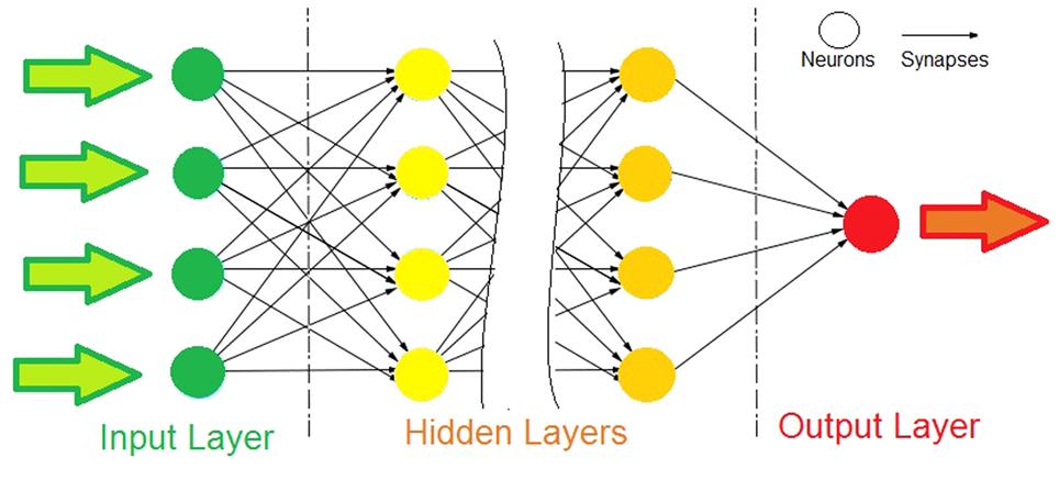
The ANNs proposed in this study have a feed-forward MLP architecture with one hidden layer. The number of input neurons is equal to the number of network input parameters, the number of hidden neurons is optimized by means of trial and error, and finally there is only an output neuron because for each investigated output a dedicated network is developed. This allows one to optimize the ANN’s generation and performance. Each ANN is trained through the Levenberg–Marquardt back-propagation algorithm combined with Bayesian regularization. The neurons’ transfer function is sigmoidal for the hidden layer and linear for the output one. A similar ANN architecture was used in previous studies regarding building energy performance simulation with excellent outcomes (Magnier and Haghighat, 2010; Paudel et al., 2014; Asadi et al., 2014; Melo et al., 2014; Buratti et al., 2014). The training stop criterion is either the stabilization of the root mean squared error or the achievement of 1000 epochs, as done by Paudel et al. (2014). The networks’ reliability is tested on a further sample of input and output data provided by the original model, and is characterized by assessing the coefficient of regression (R) and the discrepancy between the networks and the original model. In this regard, EnergyPlus simulations provide, after the MATLAB postprocess, the original model’s targets for training and testing the networks. EnergyPlus has been chosen as the BPS tool for its high reliability and capability in predicting energy performance, which is highly accredited at the international level (Ascione et al., 2015c). The adopted ratio between the numbers of sampled cases (i.e., the sizes) of training and testing sets, respectively, is 9/1 as done in previous similar studies (Magnier and Haghighat, 2010; Asadi et al., 2014). On the other hand, the size of the training set must be carefully set depending on ANN architecture and peculiarities of the explored case study; as stated by Conraud (2008), the minimum reliable value of this size is equal to (5 × number of inputs ×number of outputs).
To reach the two aforementioned main goals of this study, the proposed methodology uses the described ANNs’ architecture and presents a multistage framework to optimize the generation of the networks. In particular, it can be subdivided in the following three stages, which are elucidated in the next paragraphs:
STAGE I. The novel methodology provided by Mauro et al. (2015) is employed to investigate an established building category by carrying out SLABE. This allows identification of the parameters (related to existing stock and ERMs) that most affect building energy requests for space conditioning.
STAGE II. A first group of ANNs is generated to predict energy demand for space conditioning, and thus GCsc, of the category’s members in their current configurations. The most influential parameters concerning the existing stock, identified in Stage I, are adopted as the networks’ inputs.
STAGE III. A second group of ANNs is generated to predict energy demand for space conditioning, and thus GCsc, of the refurbished buildings, and thus when ERMs are applied to the category’s members. A dedicated ANN is developed to assess the impact of PV systems by evaluating dGCpv. The most influential parameters concerning both existing buildings and ERMs, identified in Stage I, are adopted as the networks’ inputs. This stage allows assessment of the global cost savings produced by different ERMs, and their combinations, for any category’s member with a minimum computational time. Thus, the integration of this stage with optimization procedures would imply a fast, robust, and reliable way to find the optimal—in particular, the cost-optimal—energy retrofit solutions.
11.2.1 Stage I: Simulation-Based Large-Scale Analysis of Building Energy Performance (SLABE)
In this stage, the SLABE methodology is applied to an examined building category to identify the inputs of the ANNs that are generated in the following stages. Such inputs are parameters related to the whole building system that affect the energy performance of existing buildings and proposed ERMs. Thus, they concern building geometry, envelope, operation, and energy systems. It is underlined that the proper selection of these inputs by means of SLABE is fundamental to maximize the networks’ reliability, because this strongly depends on the selected inputs (Kalogirou and Bojic, 2000). In this regard, the application of SLABE is briefly described in this paragraph and thoroughly detailed in Mauro et al. (2015) to which the reader can refer for a complete overview.
Most notably, SLABE allows one to conduct a preliminary investigation of the building category energy performance by carrying out uncertainty (UA) and sensitivity analyses (SA). The category is defined by identifying a set of characteristic parameters, denoted as pi, that affect the energy demands for space conditioning, related to geometry, thermal envelope, operation and HVAC (heating, ventilating, and air-conditioning) systems. Thus, the UA is performed to set the ranges of variability and the probabilistic distribution types of these parameters within the category, thereby identifying the sample space to be spanned. Hence, the technique of Latin hypercube sampling (LHS) is employed to generate a representative building sample (RBS), which is a group of theoretical building models that represents the energy performance, concerning space conditioning, of the whole category. EnergyPlus simulations and MATLAB postprocessing are conducted to assess the energy demands of each member of the RBS. Then, the SA is performed to find the most influential parameters on energy demands both for space heating and space cooling, which represent the outputs of the two ANNs (first group) developed in stage II (each ANN has an output), as detailed in the following paragraph. More in detail, the sensitivity index standardized rank regression coefficient (SRRC) is evaluated for each parameter pi in relation to the mentioned outputs. If the absolute value of the SRRC is bigger than a threshold value, the parameter is included among the inputs of the ANN associated to the considered output; otherwise, it is excluded. The threshold value is set in correspondence of a clear cutoff in the number of parameters versus the sensitivity index amplitude, as done by Eisenhower et al. (2012a). A similar procedure is carried out to identify the most efficient and effective ERMs. In particular, several ERMs are investigated, thereby introducing further characteristic parameters, denoted as mi, which enhance the sample space. Thus, LHS is used again to generate a second building sample (RBSretrofit) that has to represent the energy performance of the refurbished category’s members when the explored ERMs are applied. As done for the RBS, EnergyPlus simulations and MATLAB postprocessing are conducted, followed by the SA. In this case, the SRRC is evaluated for each parameter mi, associated with a certain ERM, in relation to the energy demands for space heating and cooling, respectively. The analysis of the SRRCs and MATLAB postprocess allow identification of the most efficient ERMs, and the associated parameters mi are set as additional inputs, besides the parameters pi previously screened, for the first two ANNs of the second group (Stage III). These networks are addressed to predict energy demand for space heating and cooling of refurbished buildings. In addition, a third ANN is developed to assess the electricity produced by photovoltaic (PV) systems and consumed by the facility (ELpv). Among the proposed ERMs, only photovoltaics are considered as completely renewable systems, since, at the building level, they largely represent the most profitable RES in Europe (Hamdy et al., 2013), and especially in Italy because of favorable climatic conditions (Ascione et al., 2015c). To detect the inputs of this ANN, the SRRCs are assessed for all parameters pi and mi in relation to ELpv. A parameter is included among the network’s inputs, if the absolute value of the related SRRC is bigger than the aforementioned threshold value. Definitely, the described procedure based on SLABE implies a proper, robust, and dedicated development of each network, thereby optimizing ANNs’ performances.
11.2.2 Stage II: Development of ANNs to Assess the Energy Performance of Existing Buildings
In this stage, a first group of two ANNs is defined to pursue the first goal of the study:
GOAL I. Assessing the global cost required by space conditioning (GCsc) for any category’s member in its current configuration (as is)
For this purpose, two independent ANNs are developed, both of which aim to predict a single output with reference to the present configurations of the category’s members (existing stock), and respectively:
![]() the primary energy consumption for space heating (ANN for PECh [Wh/m2 a])
the primary energy consumption for space heating (ANN for PECh [Wh/m2 a])
![]() the electric energy consumption for space cooling (ANN for ELc [Wh/m2 a]).
the electric energy consumption for space cooling (ANN for ELc [Wh/m2 a]).
More in detail, PECh means the predicted annual request of primary energy for microclimatic control in the heating season, whereas ELc means the predicted annual request of electricity for microclimatic control in the cooling season. Both indicators are calculated per unit of conditioned area to achieve more representative outcomes that are easily interpreted.
PECh and ELc are chosen as ANNs’ outputs because they allow an immediate assessment of the operating costs for space heating and cooling, respectively, by considering the specific energy prices, e.g., the price of natural gas per Nm3 or of electricity per kWhel, which are assumed constant in this study. Definitely, the operating costs for space conditioning provide the most difficult component of GCsc to be calculated, because their reliable assessment requires dynamic energy simulations. Common approaches use computationally expensive BPS tools that are here replaced by the developed ANNs with a huge reduction of simulation times, which are thus faster but still reliable energy predictions. Once the total operating cost for space conditioning (heating+cooling) from PECh and ELc is assessed, the final goal of this stage, that is the value of GCsc for any category’s member, is assessed by means of MATLAB postprocessing, according to the guidelines of the EPBD recast (EU Commission and Parliament, 2010; EU Commission, Commission Delegated Regulation EU No. 244/2012, 2012). It is highlighted that GCsc includes, besides operating costs, other components whose evaluation is much simpler without needing energy simulations; in particular, the initial investment and the replacement costs. Therefore, these components are easily assessed in MATLAB. It is highlighted that the operating costs as well as the global cost are not directly chosen as ANNs’ outputs in order to make the networks independent from the specific energy prices and the investment or replacement costs, which obviously can vary. This makes the methodology more general.
The inputs of the two ANNs differ and are set on the basis of the outcomes provided by SLABE in Stage I as described in the previous section. This ensures a dedicated development of each network thereby optimizing the performance of such surrogate models (Kalogirou and Bojic, 2000). On the other hand, the ANNs are trained and tested by using the same sampling sets, whose sizes are set by considering the network with more inputs. The use of more ANNs with one output neuron yields lower computational burden and higher reliability compared to the use of one ANN with more output neurons (Boithias et al., 2012). Indeed, this choice allows a dedicated, ad hoc selection of the inputs of each network, thereby implying smaller training sets and improving metamodeling reliability, since only the parameters that really influence an output are set as inputs of the related network. Definitely, this provides a further reason for employing two independent ANNs for the prediction of PECh and ELc, respectively, instead of a single ANN for the direct prediction of GCsc, which is the final goal of this stage.
11.2.3 Stage III: Development of ANNs to Assess the Impact of ERMs
In this stage, a second group of three ANNs is developed pursue the second goal of the study:
GOAL II. Assessing the value of GCsc for any refurbished category’s member when ERMs are applied for the reduction of space-conditioning energy needs; furthermore, also the savings dGCpv produced by the implementation of PV systems shall be predicted in conjunction with the other investigated ERMs.
For this purpose, three independent ANNs are developed, each of which aims to predict a single output with reference to the refurbished configurations of the category’s members (renovated stock), and respectively:
![]() the primary energy consumption for space heating (ANN for PECh [Wh/m2 a])
the primary energy consumption for space heating (ANN for PECh [Wh/m2 a])
![]() the electric energy consumption for space cooling (ANN for ELc [Wh/m2 a])
the electric energy consumption for space cooling (ANN for ELc [Wh/m2 a])
![]() the electric energy produced by PV systems and consumed by the facility (ANN for ELpv [Wh/m2 a]).
the electric energy produced by PV systems and consumed by the facility (ANN for ELpv [Wh/m2 a]).
The first two ANNs have the same outputs of the networks included in the first group and allow derivation of the operating costs for space conditioning. Then, as explained for the first group, MATLAB postprocessing is performed to assess the value of GCsc for any refurbished category’s member, by considering operating, investment, and replacement costs as recommended in (EU Commission and Parliament, 2010; EU Commission, Commission Delegated Regulation EU No. 244/2012, 2012). Therefore, these two ANNs provide a prediction of the impact that proper ERMs exert on global cost for space conditioning.
Furthermore, a third ANN is introduced to evaluate the electricity produced by PV systems and consumed by the building per unit of net floor area, denoted as ELpv. This ANN allows assessment of the savings dGCpv produced by PV systems, also in presence of further ERMs, by considering the reduction of operating costs for electricity linked to the energy saving ELpv as well as the investment and replacement costs for photovoltaics. Again, the guidelines of the EPBD recast (EU Commission and Parliament, 2010; EU Commission, Commission Delegated Regulation EU No. 244/2012, 2012) are followed to calculate the global cost.
As argued for the first network group, these three ANNs are also independent in the sense that they are provided with different groups of inputs to reduce the computational burden required by the training procedure. In addition, this ensures a higher reliability compared to the generation of a single ANN with more outputs (Boithias et al., 2012). The ANNs’ inputs are set according to the results of the sensitivity analysis carried out in Stage I by means of the implementation of SLABE, as described in the Section 11.2.1. These inputs include both parameters that characterize the existing building stock (pi) and parameters associated with the implementation of ERMs (mi). Only the most influential and effective retrofit measures, found through the SA, are considered in the ANNs’ development. Considering ineffective ERMs would also be useless, since, most likely, they will not be applied because they are not convenient. This screening allows optimization of ANN generation, in terms of both required computational times and model reliability.
Finally, the ANNs of this second group adopt the same training and testing sets (clearly, different from the first group), whose sizes are set by considering the network with more inputs.
11.3 Application: An Office Case Study
For testing purposes, the methodology is applied to a real case study, i.e., office buildings built in South Italy between 1920 and 1970. This is the same building category investigated by Mauro et al. (2015) through the application of SLABE. Therefore, the results of the sensitivity analyses reported in that study are here employed to optimize the ANNs’ generation. In other words, Stage I of the methodology has been carried out in Mauro et al. (2015), and thus the outcomes shown in the next paragraphs are focused on Stages II and III, which provide the final goals of this study.
The International Weather for Energy Calculations (IWEC) weather data file (Chantrelle et al., 2011) of the city of Naples is set in EnergyPlus simulations, because, with reference to South Italy, Naples is one of the main districts and presents average climatic conditions. Thus, the outcomes obtained for Naples are valid for many cities in South Italy with a good approximation.
11.3.1 Presentation of the Case Study
The investigated building category includes 8800 members (around 13% of the Italian office stock, apps1.eere.energy.gov/buildings/energyplus/weatherdata_about.cfm/). Thus, its energy renovation can provide tangible energy, economic, and environmental benefits at the national level. In the following paragraphs, the explored building stock and the proposed ERMs are briefly described. For a thorough overview, the readers can refer to Mauro et al. (2015).
11.3.1.1 Existing Building Stock
The energy performance of the category’s members in their present configurations (i.e., the existing building stock) is affected by 48 characteristic parameters (pi). In particular, these parameters are relevant to the energy requests for space conditioning. They concern building geometry, envelope, operation, and HVAC systems. As reported in Table 11.1, the variability of each parameter within the category is characterized by a type of probability distribution (uniform or normal) and a range of variability. These ranges provided the sample space that represent the whole category.
Table 11.1
Characteristic parameters (pi) of the investigated building stock: type of distribution in the stock; mean value (μ) and standard deviation (σ) for normal distributions; range of variability
| Characteristic parameters of the building stock | Distribution | μ | σ | Range | ||
| Geometry | p1 | Orientation (angle between true north and building north) | Uniform | – | – | 0°; ±30°; ±60°; 90° |
| p2 | Area of each floor (m2) | Uniform | – | – | 100÷500 | |
| p3 | Form ratio | Uniform | – | – | 1.00÷5.00 | |
| p4 | Floor height (m) | Uniform | – | – | 2.70÷4.20 | |
| p5 | Window-to-wall ratio: south | Uniform | – | – | 10%÷40% | |
| p6 | Window-to-wall ratio: east | Uniform | – | – | 10%÷40% | |
| p7 | Window-to-wall ratio: north | Uniform | – | – | 10%÷40% | |
| p8 | Window-to-wall ratio: west | Uniform | – | – | 10%÷40% | |
| p9 | Number of floors | Uniform | 1; 2; 3; 4; 5 | |||
| Envelope | p10 | Air gap thermal resistance (m2 K/W) | Normal | 0.156 | 0.01 | 0.116÷0.196 |
| p11 | External walls’ solar absorptance (a) | Normal | 0.50 | 0.20 | 0.10÷0.90 | |
| p12 | Roof solar absorptance (a) | Normal | 0.50 | 0.20 | 0.10÷0.90 | |
| p13 | Concrete (internal partitions) thickness (m) | Normal | 0.15 | 0.05 | 0.05÷0.25 | |
| p14 | Type of window glasses | Uniform | – | – | Single/double glazed | |
| p15 | Type of window frames | Uniform | – | – | Wood/aluminum | |
| p16 | Clay (floor) thickness (m) | Normal | 0.06 | 0.2 μ | (μ–3σ)÷(μ+3σ) | |
| p17 | Clay (floor) thermal conductivity (W/m K) | Normal | 0.12 | 0.2 μ | (μ–3σ)÷(μ+3σ) | |
| p18 | Clay (floor) density (kg/m3) | Normal | 450 | 0.2 μ | (μ–3σ)÷(μ+3σ) | |
| p19 | Clay (floor) specific heat (J/kg K) | Normal | 1200 | 0.2 μ | (μ–3σ)÷(μ+3σ) | |
| p20 | Expanded clay (roof) thickness (m) | Normal | 0.05 | 0.2 μ | (μ–3σ)÷(μ+3σ) | |
| p21 | Expanded clay (roof) thermal conductivity (W/m K) | Normal | 0.27 | 0.2 μ | (μ–3σ)÷(μ+3σ) | |
| p22 | Expanded clay (roof) density (kg/m3) | Normal | 900 | 0.2 μ | (μ–3σ)÷(μ+3σ) | |
| p23 | Expanded clay (roof) specific heat (J/kg K) | Normal | 1000 | 0.2 μ | (μ–3σ)÷(μ+3σ) | |
| p24 | External bricks’ (walls) thickness (m) | Normal | 0.12 | 0.2 μ | (μ–3σ)÷(μ+3σ) | |
| p25 | External bricks’ (walls) thermal conductivity (W/m K) | Normal | 0.72 | 0.2 μ | (μ–3σ)÷(μ+3σ) | |
| p26 | External bricks’ (walls) density (kg/m3) | Normal | 1800 | 0.2 μ | (μ–3σ)÷(μ+3σ) | |
| p27 | External bricks’ (walls) specific heat (J/kg K) | Normal | 840 | 0.2 μ | (μ–3σ)÷(μ+3σ) | |
| p28 | Floor block thickness (m) | Normal | 0.18 | 0.2 μ | (μ–3σ)÷(μ+3σ) | |
| p29 | Floor block thermal conductivity (W/m K) | Normal | 0.66 | 0.2 μ | (μ–3σ)÷(μ+3σ) | |
| p30 | Floor block density (kg/m3) | Normal | 1800 | 0.2 μ | (μ–3σ)÷(μ+3σ) | |
| p31 | Floor block specific heat (J/kg K) | Normal | 840 | 0.2 μ | (μ–3σ)÷(μ+3σ) | |
| p32 | Internal bricks’ (walls) thickness (m) | Normal | 0.08 | 0.2 μ | (μ–3σ)÷(μ+3σ) | |
| p33 | Internal bricks’ (walls) thermal conductivity (W/m K) | Normal | 0.90 | 0.2 μ | (μ–3σ)÷(μ+3σ) | |
| p34 | Internal bricks’ (walls) density (kg/m3) | Normal | 2000 | 0.2 μ | (μ–3σ)÷(μ+3σ) | |
| p35 | Internal bricks’ (walls) specific heat (J/kg K) | Normal | 840 | 0.2 μ | (μ–3σ)÷(μ+3σ) | |
| p36 | Roof block thickness (m) | Normal | 0.22 | 0.2 μ | (μ–3σ)÷(μ+3σ) | |
| p37 | Roof block thermal conductivity (W/m K) | Normal | 0.66 | 0.2 μ | (μ–3σ)÷(μ+3σ) | |
| p38 | Roof block density (kg/m3) | Normal | 1800 | 0.2 μ | (μ–3σ)÷(μ+3σ) | |
| p39 | Roof block specific heat (J/kg K) | Normal | 840 | 0.2 μ | (μ–3σ)÷(μ+3σ) | |
| Operation | p40 | People density (people/m2) | Normal | 0.12 | 0.2 μ | (μ–2σ)÷(μ+2σ) |
| p41 | Artificial light load (W/m2) | Normal | 15 | 0.2 μ | (μ–2σ)÷(μ+2σ) | |
| p42 | Equipment load (W/m2) | Normal | 15 | 0.2 μ | (μ–2σ)÷(μ+2σ) | |
| p43 | Infiltration rate (h−1) | Normal | 0.50 | 0.2 μ | (μ–2σ)÷(μ+2σ) | |
| p44 | Heating set-point temperature (°C) | Normal | 20 | 1 | 19 ÷22 | |
| p45 | Cooling set-point temperature (°C) | Normal | 26 | 1 | 24 ÷27 | |
| HVAC | p46 | Heating terminals: Fan coils (FC)/hot water radiators (Rad) | Uniform | – | – | Fc/Rad |
| p47 | Boiler energy efficiency (η) | Uniform | – | – | 0.70 ÷0.95 | |
| p48 | Chiller energy efficiency ratio (EER) | Uniform | – | – | 2.00 ÷3.00 | |

Fig. 11.2 depicts the plan and axonometric views of a generic category’s member to facilitate the interpretation of the geometry parameters reported in Table 11.1.
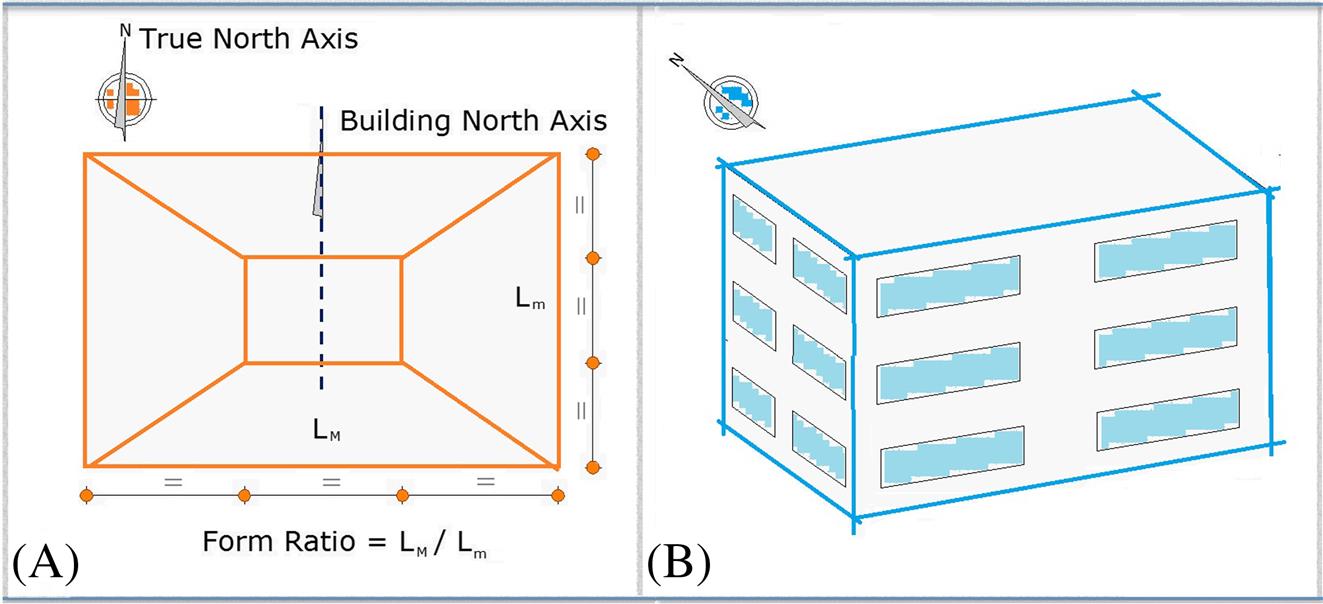
Concerning the building envelope parameters, it should be noted that the envelope components are composed of the following layers characterized by the parameters of Table 11.1 (from the external to the internal one):
The layers that exert a negligible influence on building performance (e.g., plaster, screeds, and tiles) are not considered. There are no solar shading systems. Concerning energy systems, heating is provided by a natural gas hot-water boiler, with nominal efficiency (related to the low calorific value) denoted as η. Cooling is provided by an electric air-cooled chiller, with nominal energy efficiency ratio denoted as EER.
11.3.1.2 Energy Retrofit Measures
Given the outcomes of Mauro et al. (2015), the following effective ERMs are proposed for the reduction of the energy needs linked to space conditioning:
ERM 1. Installation of a thermal insulation layer (thermal conductivity =0.040 W/m K, density =15 kg/m3, specific heat =1400 J/kg K) on the external side of external walls. The thickness (t) varies within the range 0 ÷0.12 m. The initial investment cost is given by (500 −3000 ×t) €/m3 of insulant volume (Mauro et al., 2015).
ERM 2. Installation of a thermal insulation layer (thermal conductivity =0.040 W/m K, density =15 kg/m3, specific heat =1400 J/kg K) on the external side of the roof. The thickness (t) varies within the range 0 ÷0.12 m. The initial investment cost is given by (500 −3000 ×t) €/m3 of insulant volume (Mauro et al., 2015).
ERM 3. Installation of a new plastering on the roof characterized by a low value of solar absorptance (a = 0.05). The initial investment cost is given by 20 €/m2 of roof area (Mauro et al., 2015).
ERM 4. Installation of new argon-filled double-glazed windows with low-emissivity (low-e) coatings and PVC frames (windows’ thermal transmittance Uw=1.8 W/m2 K). The initial investment cost is given by 250 €/m2 of windows’ area (Mauro et al., 2015).
ERM 5. Installation of external solar shading systems, composed by diffusive blinds. Both solar and visible transmittances are set equal to 0.5 and the solar set-point (total solar radiation) is assumed equal to 450 W/m2. The initial investment cost is given by 50 €/m2 of windows’ area (Mauro et al., 2015).
ERM 6. Implementation of a free cooling strategy during the cooling season by means of mechanical ventilation systems. The initial investment cost is given by 10 €/m2 of conditioned area (Mauro et al., 2015).
ERM 7. Installation of a natural gas hot-water condensing boiler with nominal η = 1.06 and thermal capacity Pt (kW) that varies in function of the considered category’s member. The initial investment cost is given by (80 ×Pt+1900) € (Mauro et al., 2015).
ERM 8. Installation of an electric water-cooled chiller (+cooling tower) with nominal EER =5.00 and thermal capacity Pf (kW) that varies in function of the considered category’s member. The initial investment cost is given by (250 ×Pf + 8000) € (Mauro et al., 2015).
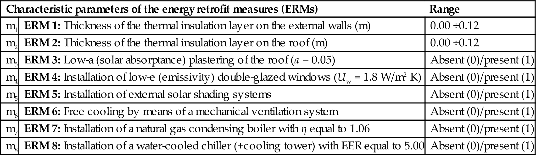
Each ERM is defined by a characteristic parameter (mi), as reported in Table 11.2. For the first two ERMs, the parameters are continuous and express the insulation layer thickness. Conversely, for the other ERMs the parameters are Boolean (it can be equal to either 0 or 1) and express the absence (0) or the presence (1) of the associated measures.
Table 11.2
Characteristic parameters (mi) of the ERMs for the reduction of the energy needs linked to space conditioning and associated ranges of variability
| Characteristic parameters of the energy retrofit measures (ERMs) | Range | |
| m1 | ERM 1: Thickness of the thermal insulation layer on the external walls (m) | 0.00 ÷0.12 |
| m2 | ERM 2: Thickness of the thermal insulation layer on the roof (m) | 0.00 ÷0.12 |
| m3 | ERM 3: Low-a (solar absorptance) plastering of the roof (a = 0.05) | Absent (0)/present (1) |
| m4 | ERM 4: Installation of low-e (emissivity) double-glazed windows (Uw = 1.8 W/m2 K) | Absent (0)/present (1) |
| m5 | ERM 5: Installation of external solar shading systems | Absent (0)/present (1) |
| m6 | ERM 6: Free cooling by means of a mechanical ventilation system | Absent (0)/present (1) |
| m7 | ERM 7: Installation of a natural gas condensing boiler with η equal to 1.06 | Absent (0)/present (1) |
| m8 | ERM 8: Installation of a water-cooled chiller (+cooling tower) with EER equal to 5.00 | Absent (0)/present (1) |
In addition, a last ERM (ERM 9) is proposed to consider the installation of polycrystalline photovoltaic (PV) panels on the building roof. Clearly, this ERM does not merely affect the energy needs for space conditioning but the total demand of electricity. Therefore, it is investigated separately. PV panels are oriented to the south and the tilt angle is equal to 34 degrees to maximize the annual production of electricity (Mauro et al., 2015; PV-GIS Software). The conversion efficiency is 14%. This ERM is characterized by a continuous parameter that expresses the size of PV systems by indicating the percentage of the roof area covered by PV panels.
Finally, the renovated building stock is characterized by 57 parameters (48 pi + 9 mi).
Further ERMs were explored by Mauro et al. (2015), but they are not considered here because they are not energy and/or cost effective as shown through the application of SLABE.
11.3.2 Results and Discussion
This section illustrates the results provided by the proposed methodology concerning the examined category, i.e., the office building stock built in South Italy between 1920 and 1970. The attention is focused on Stages II and III, since Stage I was already performed for this building category in Mauro et al. (2015).
It is outlined that, in global cost assessments, the specific prices of electricity and natural gas are considered constant and set equal to 0.25 €/kWhel and 0.90 €/Nm3, respectively (http://www.energy.eu/). Moreover, the calculation period is assumed equal to 20 years, as recommended for non-residential buildings (EU Commission and Parliament, 2010; EU Commission, Commission Delegated Regulation EU No. 244/2012, 2012).
11.3.2.1 Existing Building Stock
As elucidated in the Section 11.2, the first main goal of this study is:
GOAL I. Assessing the global cost required by space conditioning (GCsc) for any category’s member in its current configuration (as is).
For this purpose, two independent ANNs are developed, both of which aim to predict a single output with reference to existing buildings (as is), and respectively:
![]() the primary energy consumption for space heating (ANN for PECh)
the primary energy consumption for space heating (ANN for PECh)
![]() the electric energy consumption for space cooling (ANN for ELc).
the electric energy consumption for space cooling (ANN for ELc).
The outcomes of these ANNs are employed to assess the value of GCsc for each investigated building model by means of MATLAB postprocessing.
The two ANNs are related to the existing building stock, which is characterized by the 48 parameters of Table 11.1. Thus, the inputs of the networks are chosen among these parameters, based on the outcomes provided by the sensitivity analysis (SA) performed in Stage I (proposed in Mauro et al., 2015) by applying SLABE. The threshold value of the sensitivity index SRRC for parameter selection is set equal to 0.05. Finally, the found groups of inputs for the two ANNs are shown in Table 11.3.
Table 11.3
Parameters chosen as inputs of the ANNs for the prediction of primary energy consumption for space heating (PECh) and electricity consumption for space cooling (ELc) concerning the existing building stock
| Existing building stock: ANNs’ inputs ( |
ANN for PECh | ANN for ELc | ||
| Geometry | p1 | Orientation (angle between true north and building north) | ||
| p2 | Area of each floor (m2) | |||
| p3 | Form ratio | |||
| p4 | Floor height (m) | |||
| p5 | Window-to-wall ratio: South | |||
| p6 | Window-to-wall ratio: East | |||
| p7 | Window-to-wall ratio: North | |||
| p8 | Window-to-wall ratio: West | |||
| p9 | Number of floors | |||
| Envelope | p11 | External walls’ solar absorptance (a) | ||
| p12 | Roof solar absorptance (a) | |||
| p14 | Type of window glasses | |||
| p16 | Clay (floor) thickness (m) | |||
| p17 | Clay (floor) thermal conductivity (W/m K) | |||
| p24 | External bricks’ (walls) thickness (m) | |||
| p25 | External bricks’ (walls) thermal conductivity (W/m K) | |||
| p32 | Internal bricks’ (walls) thickness (m) | |||
| p33 | Internal bricks’ (walls) thermal conductivity (W/m K) | |||
| p36 | Roof block thickness (m) | |||
| p37 | Roof block thermal conductivity (W/m K) | |||
| Operation | p40 | People density (people/m2) | ||
| p41 | Artificial light load (W/m2) | |||
| p42 | Equipment load (W/m2) | |||
| p43 | Infiltration rate (h−1) | |||
| p44 | Heating set-point temperature (°C) | |||
| p45 | Cooling set-point temperature (°C) | |||
| HVAC | p46 | Heating terminals: fan coils (FC)/hot water radiators (Rad) | ||
| p47 | Boiler energy efficiency (η) | |||
| p48 | Chiller energy efficiency ratio (EER) | |||
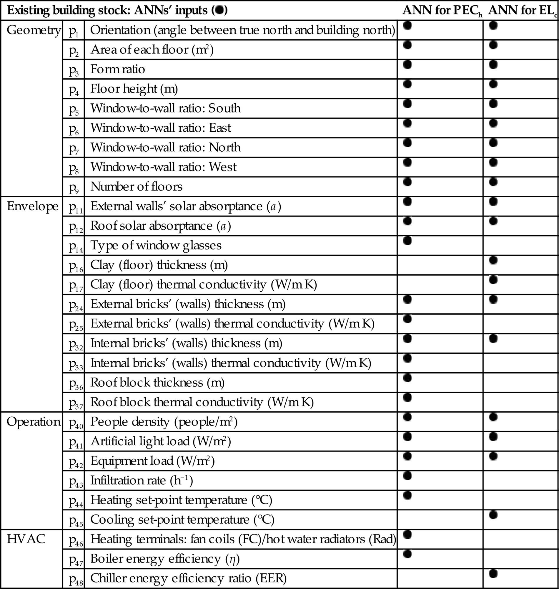
Negligible parameters, not selected as ANNs’ inputs, are not reported.
LHS is performed to generate a sample S1 of 500 building models. The sample space is defined by the inputs of the two networks (see Table 11.3) for a total of 29 parameters. This size of S1 has been set in order to generate a representative sample of the whole existing building stock (Mauro et al., 2015). Then, EnergyPlus simulations and MATLAB postprocessing are performed to evaluate PECh, ELc, and thus GCsc for the 500 building models (sampled cases). This provides a set of 500 values of GCsc, which represent the simulated targets. As described in Section 11.2, for the networks’ generations, the adopted ratio between the sizes of training and testing sets is 9/1. Therefore, the training set is built by collecting 450 cases of S1 (thereby respecting the minimum value recommended by Conraud, 2008), while the testing set collects the remaining 50 cases.
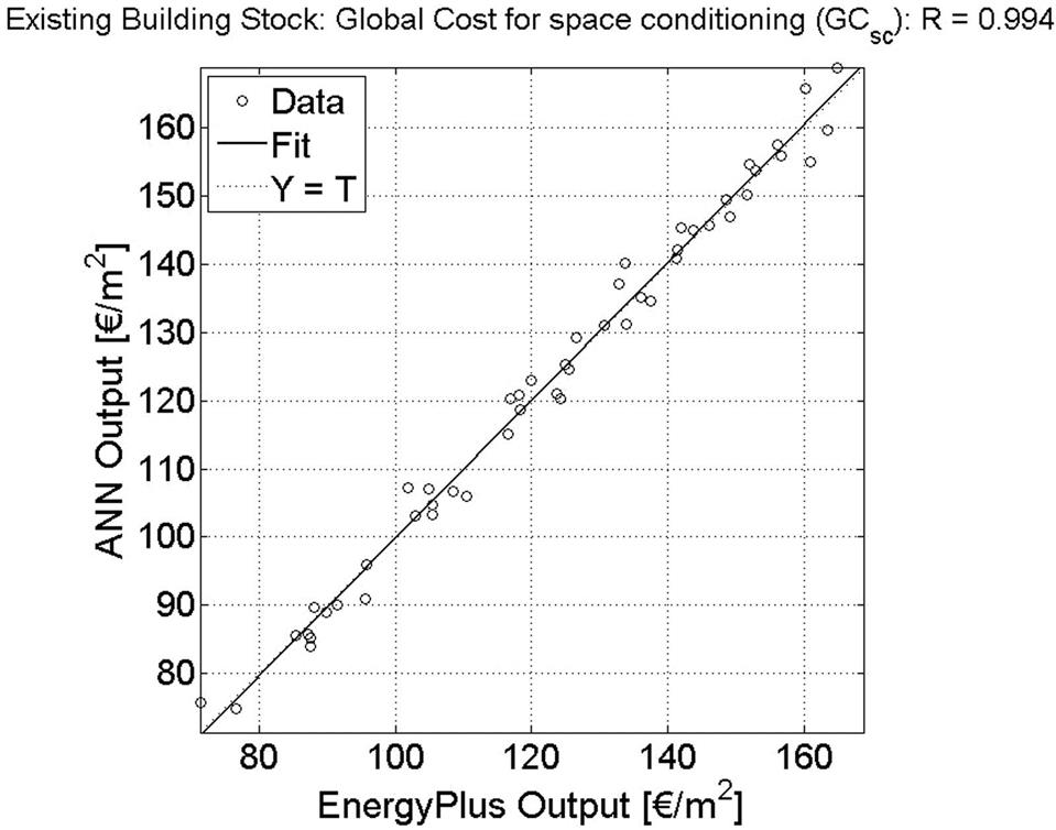
The performance of this first ANN group is assessed by considering the regression (Fig. 11.3) and the distribution of the relative errors (Fig. 11.4) compared to the EnergyPlus simulated targets, with reference to the final goal GCsc. The outcomes are very satisfactory. The regression coefficient (R) is equal to 0.994 and the average (within the testing test) of the absolute values of relative errors is 1.91%.

11.3.2.2 Impact of ERMs on Global Cost
As elucidated in the Section 11.2, the second main goal of this study is:
GOAL II. Assessing the value of GCsc for any refurbished category’s member when energy retrofit measures (ERMs) are applied for the reduction of space-conditioning energy needs; furthermore, also the global cost savings (dGCpv) produced by the implementation of photovoltaic (PV) systems shall be predicted in conjunction with the other investigated ERMs.
For this purpose, three independent ANNs are developed, each of which aims to predict a single output with reference to the refurbished buildings, and respectively:
![]() the primary energy consumption for space heating (ANN for PECh)
the primary energy consumption for space heating (ANN for PECh)
![]() the electric energy consumption for space cooling (ANN for ELc)
the electric energy consumption for space cooling (ANN for ELc)
![]() the electric energy produced by PV systems and consumed by the facility (ANN for ELpv).
the electric energy produced by PV systems and consumed by the facility (ANN for ELpv).
By performing MATLAB postprocessing for each investigated refurbished building model, the outcomes of the first two ANNs are employed to assess the value of GCsc, while the outcome of the third ANN is used to predict the value of dGCpv.
The three ANNs are related to the renovated building stock (when one or more of the nine proposed ERMs are applied), which is characterized by 57 parameters as argued in the Section 11.3.1.2. These parameters define both the energy peculiarities of the category’s members (parameters pi) and the ERMs (parameters mi). As done for the first ANN group, the inputs of the networks are chosen among these parameters, based on the outcomes provided by the SA of Stage I (proposed in Mauro et al., 2015). The first two networks have the same inputs of the corresponding networks of the first group as concerns the parameters pi (Table 11.3), whereas the inputs related to the parameters mi are shown in Table 11.4. Conversely, the third ANN, which addresses the prediction of PV systems’ performance, presents only three inputs: the building form ratio, the number of floors and the photovoltaics’ size, which is expressed by the percentage of the roof area covered by polycrystalline PV panels. The first two parameters have an impact on the fraction of the electricity that is produced by the PV systems and consumed by the building, while the third parameter clearly affects the PV production of electricity.
Table 11.4
Additional parameters chosen as inputs of the ANNs related to the renovated building stock in order to consider the implementation of the proposed energy retrofit measures (ERMs) for the reduction of space-conditioning energy needs
| Energy retrofit measures: ANNs’ inputs ( |
ANN for PECh | ANN for ELc | |
| m1 | ERM 1: Thickness of the thermal insulation layer on the external walls (m) | ||
| m2 | ERM 2: Thickness of the thermal insulation layer on the roof (m) | ||
| m3 | ERM 3: Low-a (solar absorptance) plastering of the roof (a=0.05) | ||
| m4 | ERM 4: Installation of low-e (emissivity) double-glazed windows (Uw=1.8 W/m2 K) | ||
| m5 | ERM 5: Installation of external solar shading systems | ||
| m6 | ERM 6: Free cooling by means of a mechanical ventilation system | ||
| m7 | ERM 7: Installation of a natural gas condensing boiler with η equal to 1.06 | ||
| m8 | ERM 8: Installation of a water-cooled chiller (+cooling tower) with EER equal to 4.80 | ||

LHS is performed again to generate a second sample S2 of 1000 refurbished building models. The sample space is defined by the inputs of the three networks for a total of 38 parameters. S2 is bigger than S1 because additional parameters are investigated, and therefore the size is doubled in order to reliable represent the impact of the proposed ERMs. EnergyPlus simulations and MATLAB postprocessing are performed to evaluate PECh, ELc, and thus GCsc, as well as ELpv, and thus dGCpv, for the 1000 sampled cases. This provides a set of 1000 values of GCsc, which represent the simulated targets of the first two ANNs (addressed to space conditioning), and a further set of 1000 values of dGCpv, which represent the simulated targets of the third ANN (addressed to PV). Also in this case, the adopted ratio between the sizes of training and testing sets is 9/1. Therefore, the training set is built by collecting 900 cases of S2 (respecting the minimum value recommended by Conraud, 2008), while the testing set collects the remaining 100 cases.
The performances of the ANNs are assessed by considering the regression and the distribution of the relative errors compared to EnergyPlus simulated targets, with reference to the final goals, namely GCsc (Figs. 11.5 and 11.6) and dGCpv (Figs. 11.7 and 11.8).


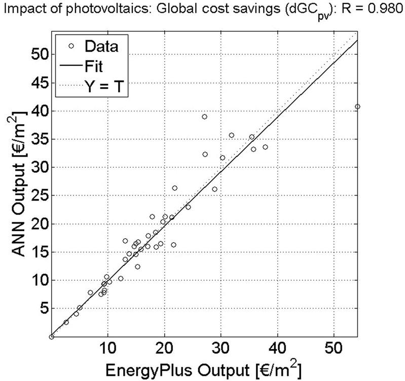
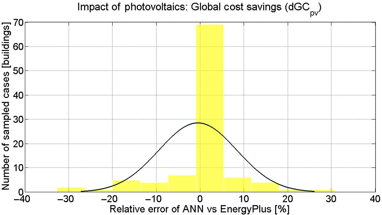
The outcomes are summarized in Table 11.5, where they are also compared to those achieved for the first network group. Naturally, the performance of this second group is slightly worse, because a more complex and heterogeneous sample space is explored. However, also for this group, the metamodeling reliability is very high: the regression coefficient (R) is equal to 0.988 for GCsc prediction and 0.980 for dGCpv prediction, and the averages (within the testing set) of the absolute values of relative errors are equal to 3.84% and 4.42%, respectively. Definitely, the developed ANNs ensure a reliable and punctual prediction of energy performance and retrofit potentials, concerning the impact of proper ERMs on building global cost, of any member of a certain category, by producing, at the same time, a drastic reduction (around 98%, as shown in the following paragraph) of computational times.
Table 11.5
Performance and reliability indices of the developed ANNs within the testing set
| R | Number of cases with absolute value of relative error | Average of the of | relative errors| | |||||
| <1% | <2.5% | <5% | <10% | <25% | |||
| Prediction of GCsc for existing buildings | 0.994 | 36% | 76% | 96% | 100% | 100% | 1.91% |
| Prediction of GCsc in presence of ERMs | 0.988 | 20% | 42% | 67% | 96% | 100% | 3.84% |
| Prediction of dGCpv due to PV panels | 0.980 | 63% | 65% | 71% | 82% | 97% | 4.42% |

Finally, Figs. 11.9 and 11.10 are proposed to outline that the ERMs actually produce significant global cost savings within the testing set, which represents the whole category. In particular, the histograms of Fig. 11.9 show that the implementation of the ERMs for the reduction of space-conditioning energy needs yields quite low values of GCsc (lower that 100 €/m2) for a wide segment of the testing set. In detail, the average reduction of GCsc is around 15 €/m2.

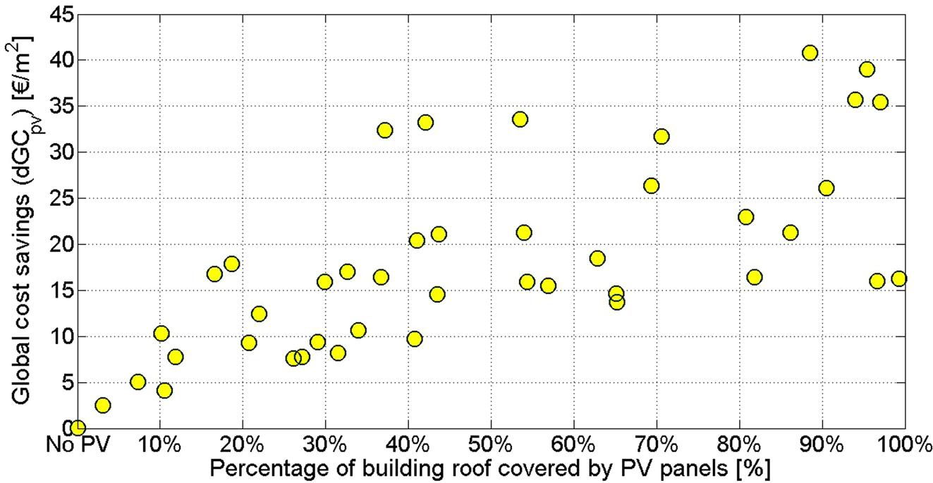
Lastly, Fig. 11.10 shows how the size of photovoltaic systems affect the global cost saving dGCpv. The cost-optimal size is provided by a percentage of covered roof area around 85–95%. The resulting global cost savings is about 40 €/m2.
11.4 Integration of the ANNs in Optimization Procedures to Optimize Energy Retrofit Design
As argued in the Introduction, a building is a very complex system consisting of highly interactive components (envelope, devices, occupants, etc.). Therefore, the prediction of building energy performance is very arduous and requires the adoption of proper BPS tools that run dynamic energy simulations. However, BPS tools are quite time-consuming and, definitely, this issue is amplified when several simulations are needed, as occurs for cost-optimal analyses or BPO procedures that aim to find optimal building retrofit solutions.
This computational issue can be solved by coupling the optimization algorithms with surrogate models, which replace the BPS tools, thereby drastically reducing the required computational times for an effective and robust building energy design. To that end, Li et al. (2010) proposed a wide review where the most important techniques are shown as well as their applications; such metamodeling techniques are compared as tools for supporting optimization and decision-making. Regarding BPO, some previous studies proposed interesting coupling schemes (Magnier and Haghighat, 2010; Li et al., 2010; Hopfe et al., 2012; Tresidder et al., 2012; Eisenhower et al., 2012b; Asadi et al., 2014), by combining, for instance, genetic algorithms with ANNs (Magnier and Haghighat, 2010; Asadi et al., 2014), SVR (Eisenhower et al., 2012b), and Kriging surrogate models (Hopfe et al., 2012; Tresidder et al., 2012). However, these studies referred to single buildings, and therefore they did not completely exploit the huge potentiality of surrogate models. Indeed, a surrogate model can be compared to a Swiss Army knife. As the adoption of a Swiss Army knife is useful only if most blades are used, so the development of a surrogate model is worthwhile only if it can be fully exploited. In other words, if only one blade is needed, a simple knife is more convenient, because it is less expensive; similarly, if the energy behavior of a simple building should be investigated, the use of BPS tools is generally more convenient, because it ensures a higher accuracy and a lower computational cost.
The proposed methodology allows exploitation of the high capability of ANNs because it is valid for a wide set of buildings included in the same category. Therefore, its implementation in BPO procedures, aimed at identifying optimal energy retrofit designs as those provided in (Magnier and Haghighat, 2010; Diakaki et al., 2010; Chantrelle et al., 2011; Echenagucia et al., 2015; Ascione et al., 2015a, 2015b, 2015c, 2016; Wright et al., 2002; Hamdy et al., 2011; Fesanghary et al., 2012; Hamdy et al., 2013), is extremely worthwhile because it would ensure enormous savings of computational efforts and times for several buildings. Indeed, with a processor Intel Core i7 at 2.00 GHz speed, the computational time required by an EnergyPlus simulation for the investigated case studies is around 50 s, whereas that required by the ANNs’ implementation is around 1 s. Therefore, the computational time savings is around 98%. Definitely, this can tackle the main issue for a wide diffusion of rigorous and effective approaches for building energy retrofit design. In other words, the combination of the developed ANNs with BPO approaches can support the reliable, fast, ‘ad hoc’ cost-optimal analysis of the retrofit measures for each building of an established category, by ensuring huge economic benefits for the private and environmental savings for the collective. This means sustainability.
11.5 Summary of the Main Novelties, Outcomes, and Conclusions
ANNs have been used to propose a new methodology suitable for predicting the global cost related to building space conditioning (GCsc) as well as energy retrofit potentials. In detail, the methodology can be used for each member of a building category. Two groups of ANNs are generated in a MATLAB environment by adopting the outcomes of EnergyPlus simulations as targets for training and testing the networks. The first group of ANNs is used for assessing the energy performance of the existing building stock, while the second one is necessary to predict the eventual impact of applied ERMs. To that end, all levers affecting energy performance, namely the building thermal envelope, the energy systems, and the exploitation of RESs, are considered. In particular, the first two ANNs of the second group allow the prediction of GCsc savings produced by proper, well-selected ERMs for the reduction of space-conditioning energy needs. In addition, a third ANN is generated to assess the global cost savings produced by the implementation of photovoltaic panels (dGCpv) in the presence of the other ERMs. Indeed, photovoltaics is largely the most cost-effective RES at the building level (Mauro et al., 2015). The definition of the ANNs is optimized by exploiting a novel methodology developed by the authors and called simulation-based large-scale sensitivity/uncertainty analysis of building energy performance (SLABE) (Mauro et al., 2015). Most notably, the implementation of SLABE provides all necessary and preliminary information required for the considered building category, and it operates by conducting both UA and SA. In detail, SLABE allows one to find the parameters that highly affect building energy behavior as well as those associated with the most effective ERMs. Then, the detected parameters are used as inputs of the ANNs, thereby ensuring a suitable and ad hoc development of the networks.
The methodology has been applied to an important share of the Italian building stock, namely office buildings built in South Italy between 1920 and 1970 (i.e., the same building category explored in Mauro et al. (2015), where SLABE was first proposed). More in detail, in this chapter the outcomes already provided in Mauro et al. (2015) have been further used for optimizing the generation of the networks. The results show very high accuracy and reliability, which are comparable with those achieved in previous studies for single buildings, even if a more complex case study is here investigated, that is, an entire building stock. Notably:
![]() Concerning the prediction of GCsc for the existing building stock, the regression coefficient (R) between ANNs’ outputs and EnergyPlus targets is 0.994, and the average of the absolute values of relative errors is 1.91%
Concerning the prediction of GCsc for the existing building stock, the regression coefficient (R) between ANNs’ outputs and EnergyPlus targets is 0.994, and the average of the absolute values of relative errors is 1.91%
![]() Concerning the prediction of GCsc in presence of ERMs, the value of R is 0.988, and the average of the absolute values of relative errors is 3.84%
Concerning the prediction of GCsc in presence of ERMs, the value of R is 0.988, and the average of the absolute values of relative errors is 3.84%
![]() Concerning the prediction of dGCpv produced by PV panels, value of R is 0.980, and the average of the absolute values of relative errors is 4.42%.
Concerning the prediction of dGCpv produced by PV panels, value of R is 0.980, and the average of the absolute values of relative errors is 4.42%.
Definitely, the proposed methodology ensures a reliable prediction of building energy performance by implying a reduction of computational times compared to EnergyPlus, around 98%. The benefit is therefore substantial.
All told, the methodology yields a new and powerful tool for supporting rigorous approaches to the design of building energy retrofits, and thus those based on cost optimality or aimed at building optimization, in terms of energy demands, thermal comfort, etc. Of course, other methods are already available, such as those based on transient energy simulations conducted through BPS tools, but these, when applied to a large number of studies, several buildings, or several configurations of the same building, are very expensive from the point of view of the required computational power and time. Conversely the ANNs, by subrogating the traditional BPS tools, solve this computational issue by ensuring, at the same time, a good reliability. In conclusion, the proposed methodology allows a fast, reliable, and robust application of the referred-to approaches, which is fundamental for the diffusion of a deep, rigorous, and effective energy retrofit of the existing building stock.