
Chapter 3
Two-Level Factorial Design
If you do not expect the unexpected, you will not find it.
Heraclitus
If you have already mastered the basics discussed in Chapters 1 and 2, you are now equipped with very powerful tools to analyze experimental data. Thus far, we have restricted discussion to simple, comparative one-factor designs. We now introduce factorial design—a tool that allows you to experiment on many factors simultaneously. The chapter is arranged by an increasing level of statistical detail. The latter portion becomes more mathematical, but the added effort required to study these details will pay off in increased understanding of the statistical framework and more confidence when using this powerful tool.
The simplest factorial design involves two factors, each at two levels. The top part of Figure 3.1 shows the layout of this two-by-two design, which forms the square “X-space” on the left. The equivalent one-factor-at-a-time (OFAT) experiment is shown at the upper right.
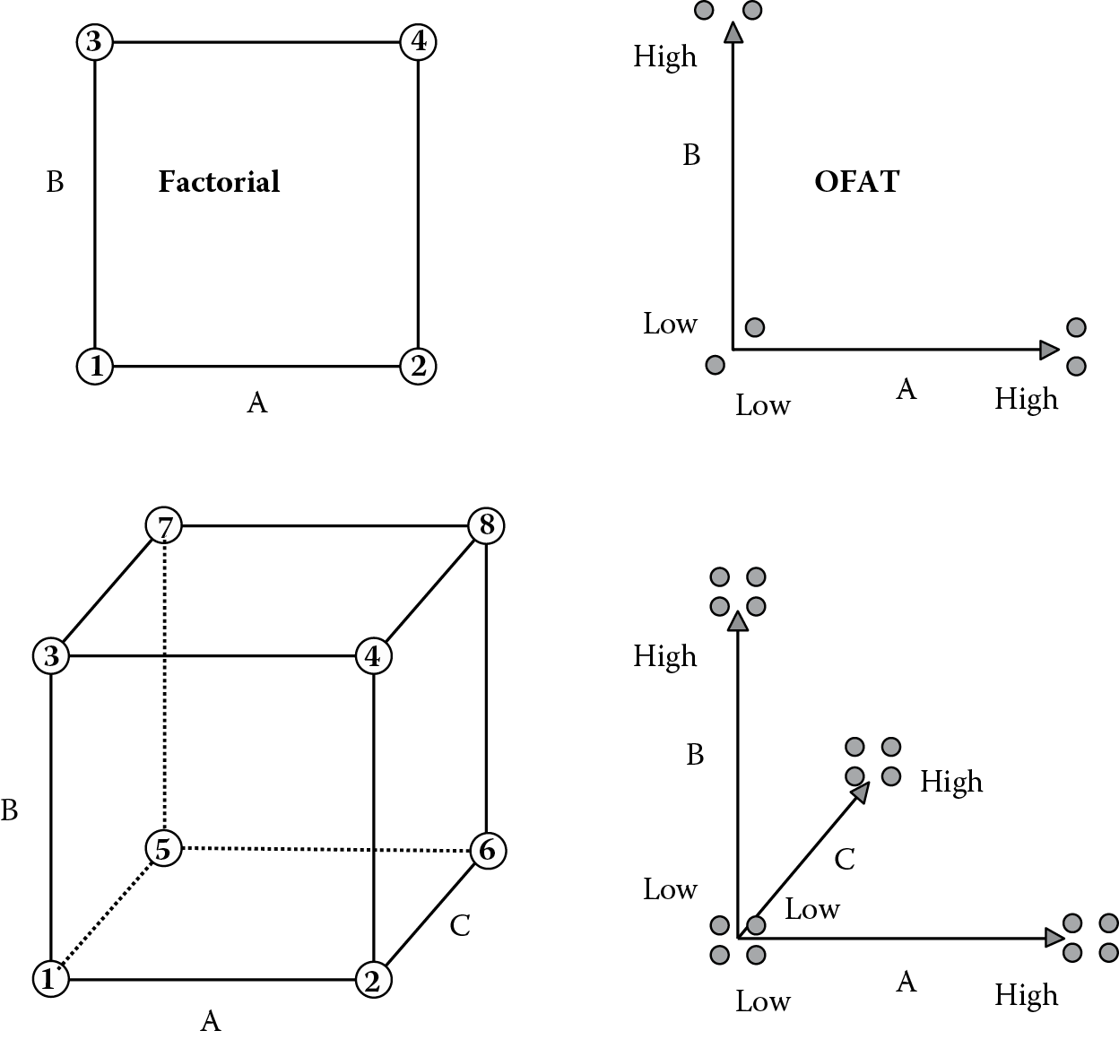
The points for the factorial designs are labeled in a “standard order,” starting with all low levels and ending with all high levels. For example, runs 2 and 4 represent factor A at the high level. The average response from these runs can be contrasted with those from runs 1 and 3 (where factor A is at the low level) to determine the effect of A. Similarly, the top runs (3 and 4) can be contrasted with the bottom runs (1 and 2) for an estimate of the effect of B.
Later, we will get into the mathematics of estimating effects, but the point to be made now is that a factorial design provides contrasts of averages, thus providing statistical power to the effect estimates. The OFAT experimenter must replicate runs to provide equivalent power. The end result for a two-factor study is that, to get the same precision for effect estimation, OFAT requires 6 runs versus only 4 for the two-level design.
The advantage of factorial design becomes more pronounced as you add more factors. For example, with three factors, the factorial design requires only 8 runs (in the form of a cube) versus 16 for an OFAT experiment with equivalent power. In both designs (shown at the bottom of Figure 3.1), the effect estimates are based on averages of 4 runs each: right-to-left, top-to-bottom, and back-to-front for factors A, B, and C, respectively. The relative efficiency of the factorial design is now twice that of OFAT for equivalent power. The relative efficiency of factorials continues to increase with every added factor.
Factorial design offers two additional advantages over OFAT:
- Wider inductive basis, i.e., it covers a broader area or volume of X-space from which to draw inferences about your process.
- It reveals “interactions” of factors. This often proves to be the key to understanding a process, as you will see in the following case study.
Two-Level Factorial Design: As Simple as Making Microwave Popcorn
We will illustrate the basic principles of two-level factorial design via an example.
What could be simpler than making microwave popcorn? Unfortunately, as everyone who has ever made popcorn knows, it’s nearly impossible to get every kernel of corn to pop. Often a considerable number of inedible “bullets” (unpopped kernels) remain at the bottom of the bag. What causes this loss of popcorn yield? Think this over the next time you stand in front of the microwave waiting for the popping to stop and jot down a list of all the possible factors affecting yield. You should easily identify 5 or even 10 variables on your own; many more if you gather several colleagues or household members to “brainstorm.”
In our example, only three factors were studied: brand of popcorn, time of cooking, and microwave power setting (Table 3.1). The first factor, brand, is clearly “categorical”—either one type or the other. The second factor, time, is obviously “numerical,” because it can be adjusted to any level. The third factor, power, could be set to any percent of the total available, so it’s also numerical. If you try this experiment at home, be very careful to do some range finding on the high level for time (see related boxed text below). Notice that we have introduced the symbols of minus (–) and plus (+) to designate low and high levels, respectively. This makes perfect sense for numerical factors, provided you do the obvious and make the lesser value correspond to the low level. The symbols for categorical factor levels are completely arbitrary, although perhaps it helps in this case to assign minus as “cheap” and plus as “costly.”
Test-factors for making microwave popcorn
|
Factor |
Name |
Units |
Low Level (–) |
High Level (+) |
|
A |
Brand |
Cost |
Cheap |
Costly |
|
B |
Time |
Minutes |
4 |
6 |
|
C |
Power |
Percent |
75 |
100 |
Two responses were considered for the experiment on microwave popcorn: taste and bullets. Taste was determined by a panel of testers who rated the popcorn on a scale of 1 (worst) to 10 (best). The ratings were averaged and multiplied by 10. This is a linear “transformation” that eliminates a decimal point to make data entry and analysis easier. It does not affect the relative results. The second response, bullets, was measured by weighing the unpopped kernels—the lower the weight, the better.
The results from running all combinations of the chosen factors, each at two levels, are shown in Table 3.2. Taste ranged from a 32 to 81 rating and bullets from 0.7 to 3.5 ounces. The latter result came from a bag with virtually no popped corn; barely enough to even get a taste. Obviously, this particular setup is one to avoid. The run order was randomized to offset any lurking variables, such as machine warm-up and degradation of taste buds.
Results from microwave popcorn experiment
|
Standard |
Run Order |
A: Brand |
B: Time (minutes) |
C: Power (percent) |
Y1 : Taste (rating) |
Y2 : “Bullets” (ounces) |
|
2 |
1 |
Costly (+) |
4 (–) |
75 (–) |
75 |
3.5 |
|
3 |
2 |
Cheap (–) |
6 (+) |
75 (–) |
71 |
1.6 |
|
5 |
3 |
Cheap (–) |
4 (–) |
100 (+) |
81 |
0.7 |
|
4 |
4 |
Costly (+) |
6 (+) |
75 (–) |
80 |
1.2 |
|
6 |
5 |
Costly (+) |
4 (–) |
100 (+) |
77 |
0.7 |
|
8 |
6 |
Costly (+) |
6 (+) |
100 (+) |
32 |
0.3 |
|
7 |
7 |
Cheap (–) |
6 (+) |
100 (+) |
42 |
0.5 |
|
1 |
8 |
Cheap (–) |
4 (–) |
75 (–) |
74 |
3.1 |
The first column in Table 3.2 lists the standard order, which can be cross-referenced to the labels on the three-factor cube in Figure 3.1. We also placed the mathematical symbols of minus and plus, called “coded factor levels,” next to the “actual” levels at their lows and highs, respectively. Before proceeding with the analysis, it will be very helpful to re-sort the test matrix on the basis of standard order, and list only the coded factor levels. We also want to dispense with the names of the factors and responses, which just get in the way of the calculations, and show only their mathematical symbols. You can see the results in Table 3.3.
Test matrix in standard order with coded levels
|
Standard |
Run |
A |
B |
C |
Y1 |
Y2 |
|
1 |
8 |
– |
– |
– |
74 |
3.1 |
|
2 |
1 |
+ |
– |
– |
75 |
3.5 |
|
3 |
2 |
– |
+ |
– |
71 |
1.6 |
|
4 |
4 |
+ |
+ |
– |
80 |
1.2 |
|
5 |
3 |
– |
– |
+ |
81 |
0.7 |
|
6 |
5 |
+ |
– |
+ |
77 |
0.7 |
|
7 |
7 |
– |
+ |
+ |
42 |
0.5 |
|
8 |
6 |
+ |
+ |
+ |
32 |
0.3 |
|
Effect Y 1 |
–1.0 |
–20.5 |
–17.0 |
66.5 |
||
|
Effect Y 2 |
–0.05 |
–1.1 |
–1.8 |
1.45 |
The column labeled “Standard” and the columns for A, B, and C form a template that can be used for any three factors that you want to test at two levels. The standard layout starts with all minus (low) levels of the factors and ends with all plus (high) levels. The first factor changes sign every other row, the second factor every second row, the third every fourth row, and so on, based on powers of 2. You can extrapolate the pattern to any number of factors or look them up in statistical handbooks.
Let’s begin the analysis by investigating the “main effects” on the first response (Y1)—taste. It helps to view the results in the cubical factor space. We will focus on factor A (brand) first (Figure 3.2).

The right side of the cube contains all the runs where A is at the plus level (high); on the left side, the factor is held at the minus level (low). Now, simply average the highs and the lows to determine the difference or contrast. This is the effect of Factor A. Mathematically, the calculation of an effect is expressed as follows:
where the ns refer to the number of data points you collected at each level. The Ys refer to the associated responses. You can pick these off the plot or from the matrix itself. For A, the effect is
In comparison to the overall spread of results, it looks like A (brand) has very little effect on taste. Continue the analysis by contrasting the averages from top-to-bottom and back-to-front to get the effects of B and C, respectively. Go ahead and do the calculations if you like. The results are –20.5 for B and –17 for C. The impact, or “effect,” of factors B (power) and C (time) are much larger than that of A (the brand of popcorn).
Before you jump to conclusions, however, consider the effects caused by interactions of factors. The full-factorial design allows estimation of all three two-factor interactions (AB, AC, and BC) as well as of the three-factor interaction (ABC). Including the main effects (caused by A, B, and C), this brings the total to seven effects; the most you can estimate from the 8-run factorial design, because one degree of freedom is used to estimate the overall mean.
Table 3.4 lists all seven effects. The main effects calculated earlier are listed in the A, B, and C columns.
Complete matrix, including interactions, with effects calculated
|
Standard |
Main Effects |
Interaction Effects |
Response |
|||||
|
A |
B |
C |
AB |
AC |
BC |
ABC |
Y1 |
|
|
1 |
– |
– |
– |
+ |
+ |
+ |
– |
74 |
|
2 |
+ |
– |
– |
– |
– |
+ |
+ |
75 |
|
3 |
– |
+ |
– |
– |
+ |
– |
+ |
71 |
|
4 |
+ |
+ |
– |
+ |
– |
– |
– |
80 |
|
5 |
– |
– |
+ |
+ |
– |
– |
+ |
81 |
|
6 |
+ |
– |
+ |
– |
+ |
– |
– |
77 |
|
7 |
– |
+ |
+ |
– |
– |
+ |
– |
42 |
|
8 |
+ |
+ |
+ |
+ |
+ |
+ |
+ |
32 |
|
Effect |
−1.0 |
−20.5 |
−17.0 |
0.5 |
−6.0 |
−21.5 |
−3.5 |
66.5 |
The pattern of pluses and minuses for interaction effects is calculated by multiplying the parent terms. For example, the AB column is the product of columns A and B, so for the first standard row, the combination of –A times –B produces +AB. Remember that numbers with like signs, when multiplied, produce a plus; whereas multiplying numbers with unlike signs produces a minus. The entire array exhibits a very desirable property of balance called orthogonality (see related sidebar in the above boxed text).
Now, it’s just a matter of computing the effects using the general formula shown previously. The results are shown on the bottom line of Table 3.4. Notice that the interaction effect of BC is even greater on an absolute scale than its parents B and C. In other words, the combination of time (B) and power (C) produces a big (negative) impact on taste. With that as a clue, look more closely at the response data (Y1). Notice the big drop-off in taste when both B and C are at their high levels. We will investigate this further after sorting out everything else.
On an absolute value scale, the other interaction effects range from near 0 (for AB) to as high as 6 (for AC). Could these just be chance occurrences due to normal variations in the popcorn, the tasting, the environment, and the like? To answer this question, let’s go back to a tool discussed at the end of Chapter 1: the normal plot. Then we can see whether some or all of the effects vary normally. Ideally, we will discover one or more effects at a significant distance from the remainder. Otherwise we have wasted a lot of experimental effort chasing noise from the system.
Before plotting the effects, it helps to convert them to absolute values, a more sensitive scale for detection of significant outcomes. The absolute value scale is accommodated via a variety of normal paper called the half-normal, which is literally based on the positive half of the full normal curve. (Imagine cutting out the bell-shaped curve and folding it in half at the mean.) As before, the vertical (y) axis of the half-normal plot displays the cumulative probability of getting a result at or below any given level. However, the probability scale for the half-normal is adjusted to account for using the absolute value of the effects.
Remember that, before plotting this data on the probability paper, you must:
- Sort the datapoints (in this case seven effects) in ascending order.
- Divide the 0 to 100% cumulative probability scale into (seven) equal segments.
- Plot the data at the midpoint of each probability segment.
In this case, each probability segment will be approximately 14.28% (100/7). The lowest weight will be plotted at 7.14%, which is the midpoint of the first segment. Table 3.5 shows this combination and all the remaining ones.
Values to plot on half-normal probability paper
|
Point |
Effect |
Absolute Value of Effect |
Cumulative Probability |
|
1 |
AB |
|0.5| |
7.14% |
|
2 |
A |
|–1.0| |
21.43% |
|
3 |
ABC |
|–3.5| |
35.71% |
|
4 |
AC |
|–6.0| |
50.00% |
|
5 |
C |
|–17.0| |
64.29% |
|
6 |
B |
|–20.5| |
78.57% |
|
7 |
BC |
|–21.5| |
92.86% |
Now all we need to do is plot the absolute values of the effect on the x-axis versus the cumulative probabilities on the specially scaled y-axis on half-normal paper (Figure 3.3).
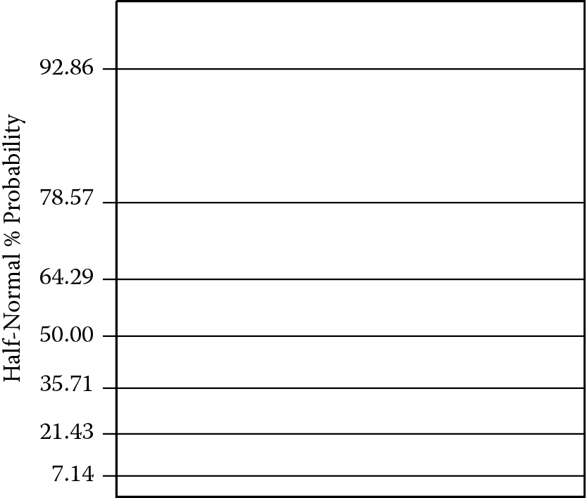
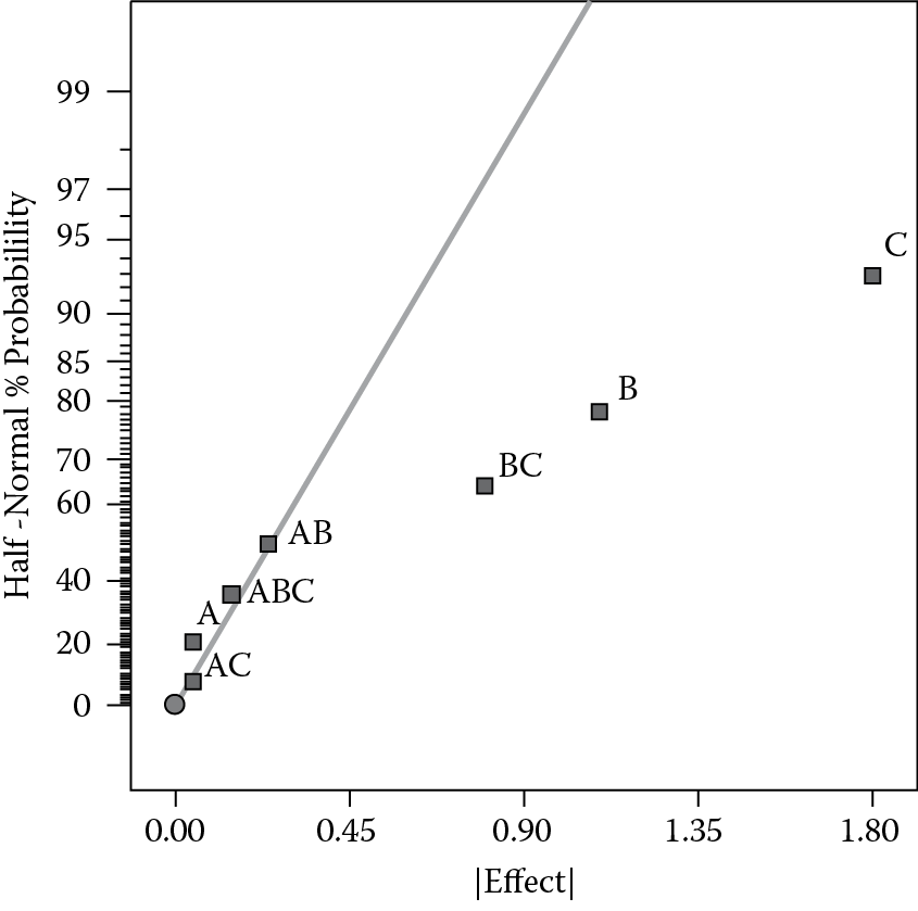
Figure 3.4 shows the completed half-normal plot for the effects on taste of popcorn. This particular graph has some features you will not usually see:

- A half-normal curve for reference
- A “dot-plot” on the x-axis representing the actual effects projected down to the x-axis number line
Notice that the biggest three effects fall well out on the tail of the normal curve (to the right). These three effects (C, B, and BC) are most likely significant in a statistical sense. We wanted to draw attention to these big effects, so we labeled them. Observe the large gap before you get to the next lowest effect. From this point on, the effects (AC, ABC, A, and AB—from biggest to smallest, respectively) fall in line, which represents the normal scatter. We deliberately left these unlabeled to downplay their importance. These four trivial effects (nearest 0) will be used as an estimate of error for the upcoming analysis of variance (ANOVA).
The pattern you see in Figure 3.4 is very typical: The majority of points fall in a line emanating from the origin, followed by a gap, and then one or more points fall off to the right of the line. The half-normal plot of effects makes it very easy to see at a glance what, if anything, is significant.
Let’s apply this same procedure to the second response for microwave popcorn: the weight of the bullets. In the last row of Table 3.6, the seven effects are calculated using the formula shown earlier:
Effects calculated for second response (bullets)
|
Standard |
A |
B |
C |
AB |
AC |
BC |
ABC |
Y2 |
|
1 |
– |
– |
– |
+ |
+ |
+ |
– |
3.1 |
|
2 |
+ |
– |
– |
– |
– |
+ |
+ |
3.5 |
|
3 |
– |
+ |
– |
– |
+ |
– |
+ |
1.6 |
|
4 |
+ |
+ |
– |
+ |
– |
– |
– |
1.2 |
|
5 |
– |
– |
+ |
+ |
– |
– |
+ |
0.7 |
|
6 |
+ |
– |
+ |
– |
+ |
– |
– |
0.7 |
|
7 |
– |
+ |
+ |
– |
– |
+ |
– |
0.5 |
|
8 |
+ |
+ |
+ |
+ |
+ |
+ |
+ |
0.3 |
|
Effect |
−0.05 |
−1.1 |
−1.8 |
−0.25 |
−0.05 |
0.80 |
0.15 |
1.45 |
Table 3.7 shows the effects ranked from low to high in absolute value, with the corresponding probabilities.
Values to plot on half-normal plot for bullets
|
Point |
Effect |
Absolute Value of Effect |
Cumulative Probability |
|
1 |
A |
|−0.05| |
7.14% |
|
2 |
AC |
|−0.05| |
21.43% |
|
3 |
ABC |
|0.15| |
35.71% |
|
4 |
AB |
|−0.25| |
50.00% |
|
5 |
BC |
|0.80| |
64.29% |
|
6 |
B |
|−1.10| |
78.57% |
|
7 |
C |
|−1.80| |
92.86% |
Notice that the probability values are exactly the same as for the previous table on taste. In fact, these values apply to any three-factor, two-level design, if you successfully perform all 8 runs and gather the response data.
Figure 3.5 shows the resulting plot (computer generated) for bullets, with all effects labeled so you can see how it’s constructed. For example, the smallest effects, A and AC, which each have an absolute value of 0.05, are plotted at 7.1 and 21.4% probability. (When effects are equal, the order is arbitrary.) Next comes effect ABC at 35.7%, and so on.
Notice how four of the effects (AB, ABC, A, and AC) fall in a line near zero. These effects evidently vary only due to normal causes—presumably as a result of experimental error (noise in the system), so they are probably insignificant. You will almost always find three-factor interactions, such as ABC, in this normal population of trivial effects. Interactions of four or more factors are even more likely to fall into this near-zero group of effects.
The effects of B, C, and BC are very big relative to the other effects. They obviously do not fall on the line. In a statistical sense, each of these three standout effects should be considered significant populations in their own right. In other words, we need to focus on factors B and C and how they interact (as BC) to affect the response of bullets.
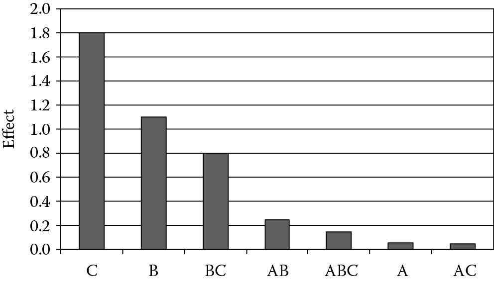
Figure 3.6 offers a simpler view of the relative effects via an ordered bar graph called a Pareto chart, which serves as a graphic representation of the principle (also called the 80/20 rule) discussed above. This becomes manifest by the vital few bars at the left towering over the trivial many on the right. (See the Appendix to this chapter for a more sophisticated form of the Pareto chart that provides statistical benchmarks for assessing statistical significance of the effects.)
A word of caution: To protect against spurious outcomes, it is absolutely vital that you verify the conclusions drawn from the half-normal plots and Pareto charts by doing an analysis of variance (ANOVA) and the associated diagnostics of “residual error.” As you will see later in this chapter, the statistics in this case pass the tests with flying colors. Please take our word on it for now. We will eventually show you how to generate and interpret all the statistical details, but it will be more interesting to jump ahead now to the effect plot.
How to Plot and Interpret Interactions
Interactions occur when the effect of one factor depends on the level of the other. They cannot be detected by traditional one-factor-at-a-time (OFAT) experimentation, so don’t be surprised if you uncover previously undetected interactions when you run a two-level design. Very often, the result will be a breakthrough improvement in your system.
The microwave popcorn study nicely illustrates how to display and interpret an interaction. In this case, both of the measured responses are greatly impacted by the interaction of time and power, so it is helpful to focus on these two factors (B and C, respectively). Table 3.8 shows the results for the two responses: taste and bullets. These are actually averages of data from Table 3.3, which we have cross-referenced by standard order. For example, the first two experiments in Table 3.3 have both time and power at their low (minus) levels. The associated taste ratings are 74 and 75, which produces an average outcome of 74.5, as shown in Table 3.4.
Data for interaction plot of microwave time versus power
|
Standard |
Time (B) |
Power (C) |
Taste (Y1 Avg) |
Bullets (Y2 Avg) |
|
1,2 |
– |
– |
74.5 |
3.3 |
|
3,4 |
+ |
– |
75.5 |
1.4 |
|
5,6 |
– |
+ |
79.0 |
0.7 |
|
7,8 |
+ |
+ |
37.0 |
0.4 |
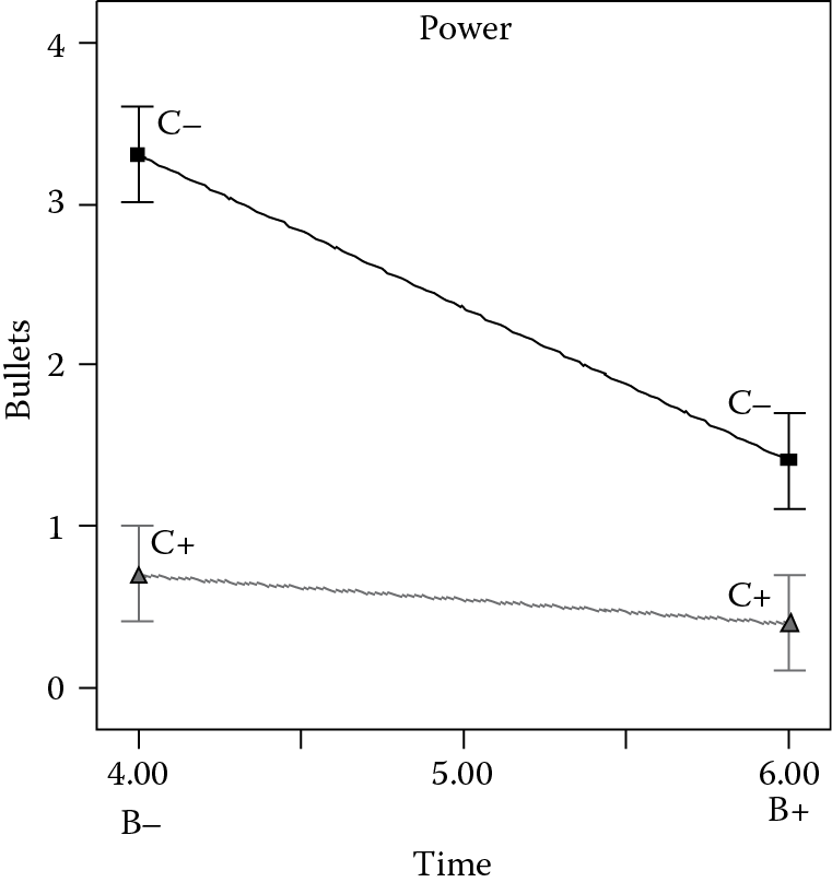
Notice that the effect of time depends on the level of power. For example, when power is low (minus), the change in taste is small—from 74.5 to 75.5. However, when power is high (plus), the taste goes very bad—from 79 to 37. This is much clearer when graphed (Figure 3.7).

Two lines appear on the plot, bracketed by least significant difference (LSD) bars at either end. The lines are far from parallel, indicating quite different effects of changing the cooking time. When power is low (C–), the line is flat, which indicates that the system is unaffected by time (B). However, when power goes high (C+), the line angles steeply downward, indicating a strong negative effect due to the increased time. The combination of high time and high power is bad for taste. Table 3.8 shows the average result to be only 37 on the 100-point rating scale. The reason is simple: The popcorn burns. The solution to this problem is also simple: Turn off the microwave sooner. Notice that when the time is set at its low level (B–), the taste remains high regardless of the power setting (C). The LSD bars overlap at this end of the interaction graph, which implies that there is no significant difference in taste.
Figure 3.8 shows how time and power interact to affect the other response, the bullets. The pattern differs from that for taste, but it again exhibits the nonparallel lines that are characteristic of a powerful two-factor interaction.
The effect of time on the weight of bullets depends on the level of power, represented by the two lines on the graph. On the lower line, notice the overlap in the least significant difference (LSD) bars at left versus right. This indicates that at high power (C+), there’s not much, if any, effect. However, the story differs for the top line on the graph where power is set at its low level (C–). Here the LSD bars do not overlap, indicating that the effect of time is significant. Getting back to that bottom line, it’s now obvious that when using the bullets as a gauge, it is best to make microwave popcorn at the highest power setting. However, recall that high time and high power resulted in a near-disastrous loss of taste. Therefore, for “multiresponse optimization” of the microwave popcorn, the best settings are high power at low time. The brand, factor A, does not appear to significantly affect either response, so choose the one that’s cheapest.
Protect Yourself with Analysis of Variance (ANOVA)
Now that we have had our fun and jumped to conclusions on how to make microwave popcorn, it’s time to do our statistical homework by performing the analysis of variance (ANOVA). Fortunately, when factorials are restricted to two levels, the procedure becomes relatively simple. We have already done the hard work by computing all the effects. To do the ANOVA, we must compute the sums of squares (SS), which are related to the effects as follows:
where N is the number of runs. This formula works only for balanced two-level factorials.
The three largest effects (B, C, and BC) are the vital few that stood out on the half-normal plot. Their sum of squares are shown in the italicized rows in Table 3.9 below. For example, the calculation for sum of squares for effect B is
ANOVA for taste
|
Source |
Sum of Squares (SS) |
Df |
Mean Square (MS) |
F Value |
Prob > F |
|
Model |
2343.0 |
3 |
781.0 |
31.5 |
<0.01 |
|
B |
840.5 |
1 |
840.5 |
34.0 |
<0.01 |
|
C |
578.0 |
1 |
578.0 |
23.3 |
<0.01 |
|
BC |
924.5 |
1 |
924.5 |
37.3 |
<0.01 |
|
Residual |
99.0 |
4 |
24.8 |
||
|
Cor Total |
2442.0 |
7 |
You can check the calculations for the sum of squares associated with effects C and BC. The outstanding effects will be incorporated in the “model” for predicting the taste response. (We provide more details on the model later.)
When added together, the resulting sum of squares provides the beginnings of the actual ANOVA. Here’s the calculation for the taste response:
The smaller effects, which fell on the near-zero line, will be pooled together and used as an estimate of error called residual. The calculation for this taste response is
The sum of squares for model and residual are shown in the first column of data in the ANOVA, shown in Table 3.9. The next column lists the degrees of freedom (df) associated with the sum of squares (derived from the effects). Each effect is based on two averages, high versus low, so it contributes 1 degree of freedom (df) for the sum of squares. Thus, you will see 3 df for the three effects in the model pool and 4 df for the four effects in the residual pool. This is another simplification made possible by restricting the factorial to two levels. The next column in the ANOVA is the mean square: the sum of squares divided by the degrees of freedom (SS/df). The ratio of mean squares (MSModel/MSResidual) forms the F value of 31.5 (= 781.0/24.8).
The F value for the model must be compared to the reference distribution for F with the same degrees of freedom. In this case, you have 3 df for the numerator (top) and 4 df for the denominator (bottom). The critical F-values can be obtained from table(s) in Appendix 1 at the back of the book by going to the appropriate column (in this case the third) and row (the fourth). Check these against the values shown in Figure 3.9.
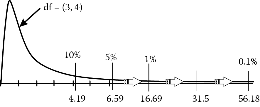
If the actual F value exceeds the critical value at an acceptable risk value, you should reject the null hypothesis. In this case, the actual F of 31.5 is bracketed by the critical values for 0.1% and 1% risk. We can say that the probability of getting an F as high as that observed, due to chance alone, is less than 1%. In other words, we are more than 99% confident that taste is significantly affected by one or more of the effects chosen for the model. That’s good.
However, we are not done yet, because it’s possible to accidentally carry an insignificant effect along for the ride on the model F. For that reason, always check each individual effect for significance. The F-tests for each effect are based on 1 df for the respective numerators and df of the residual for the denominator (in this case, 4). The critical F at 1% for these dfs (1 and 4) is 21.2. Check the appropriate table in Appendix 1 to verify this. The actual F-values for all three individual effects exceed the critical F, so we can say they are all significant, which supports the assumptions made after viewing the half-normal plot.
We haven’t talked about the last line of the ANOVA, labeled “Cor Total.” This is the total sum of squares corrected for the mean. It represents the total system variation using the average response as a baseline. The degrees of freedom are also summed, so you can be sure nothing is overlooked. In this case, we started with eight data points, but 1 df is lost to calculate the overall mean, leaving 7 df for the ANOVA.
The ANOVA for the second response, bullets, can be constructed in a similar fashion. The one shown in Table 3.10 is from a computer program that calculates the probability (p) value to several decimals (reported as “Prob > F”). The p-values are traditionally reported on a scale from 0 to 1. In this book, p-values less than 0.05 are considered significant, providing at least 95% confidence for all results. None of the p-values exceed 0.05 (or even 0.01), so we can say that the overall model for bullets is significant, as are the individual effects.
ANOVA for bullets
|
Source |
Sum of Squares |
DF |
Mean Square |
F Value |
Prob > F |
|
Model |
10.18 |
3 |
3.39 |
75.41 |
0.0006 |
|
B |
2.42 |
1 |
2.42 |
53.78 |
0.0018 |
|
C |
6.48 |
1 |
6.48 |
144.00 |
0.0003 |
|
BC |
1.28 |
1 |
1.28 |
28.44 |
0.0060 |
|
Residual |
0.18 |
4 |
0.045 |
||
|
Cor Total |
10.36 |
7 |
Let’s recap the steps taken so far for analyzing two-level factorial designs:
- Calculate effects: Average of highs (pluses) versus average of lows (minuses)
- Sort absolute value of effects in ascending order
- Lay out probability values Pi as shown by examples
- Plot effects on half-normal probability paper
- Fit line through near-zero points (“residual”)
- Label significant effects off the line (“model”)
- Calculate each effect’s sums of squares (SS) using formula
- Compute SSModel: Add SS for points far from line
- Compute SSResiduals: Add SS for points on line
- Construct ANOVA table
- Using tables, estimate the p-values for calculated F-values; if <0.05, proceed
- Plot main effect(s) and interaction(s); interpret results
We have now completed most of the statistical homework needed to support the conclusions made earlier. However, one final step must be taken for absolute protection against spurious results: Check the assumptions underlying the ANOVA.
Modeling Your Responses with Predictive Equations
This is a good place to provide details on the model tested in the ANOVA. The model is a mathematical equation used to predict a given response. To keep it simple, let’s begin the discussion by looking at only one factor. The linear model is
where Y with the circumflex or “hat” (^) is the predicted response, β0 (beta zero) is the intercept, and β1 (beta one) is the model coefficient for the input factor (X1). For statistical purposes, it helps to keep factors in coded form: –1 for low and +1 for high. As shown in Figure 3.10, changing the factor from low to high causes the measured effect on response.
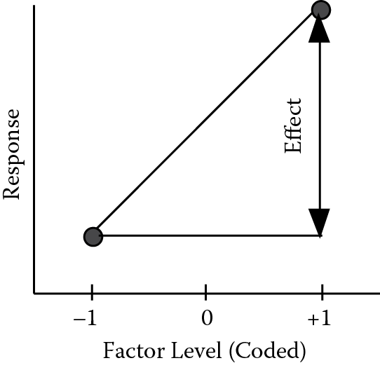
The model coefficient β1 represents the slope of the line, which is the “rise” in response (the effect) divided by the corresponding “run” in factor level (2 coded units). Therefore, the β1 coefficient in the coded model is one-half the value of the effect (effect/2).
As more factors are added, the number of terms in the model increases. The factorial model for two factors, each at two levels, is
The fitted model for the popcorn taste with the factors of time (B) and power (C) in coded form is
Taste = 66.5 − 10.25 B − 8.50 C − 10.75 BC
The value for the intercept (β0) of 66.5 represents the average of all actual responses. The coefficients can be directly compared to assess the relative impact of factors. In this case, for example, we can see that factor B (coefficient –10.25) causes a bigger effect than factor C (coefficient –8.50).
The one drawback to the coded model is that you must convert actual factor levels to coded levels before plugging in the input values. Using standard statistical regression, we produced an alternative predictive model that expresses the factors of time and power in their original units of measure:
Taste = –199 + 65 Time + 3.62 Power − 0.86 Time * Power
Use this uncoded model to generate predicted values, but don’t try to interpret the coefficients. The intercept loses meaning when you go to the uncoded model because it’s dependent on units of measure. For example, a –199 result for taste makes no sense. Similarly, in the uncoded model, you can no longer compare the coefficient of one term with another, such as time versus power.
We advise that you work only with the coded model. This is shown below for the second response:
Bullets = 1.45 − 0.55 B − 0.90 C + 0.40 BC
A good way to check your models is to enter factor levels from your design and generate the predicted response. When you compare the predicted value with the actual (observed) value, you will normally see a discrepancy. This is called the “residual.”
Diagnosing Residuals to Validate Statistical Assumptions
For statistical purposes, it’s assumed that residuals are normally distributed and independent with constant variance. Two plots are recommended for checking the statistical assumptions:
- Normal plot of residuals
- Residuals versus predicted level
Let’s look at these plots for the taste response from the popcorn experiment. Table 3.11 provides the raw data.
Residuals for taste data
|
Standard |
B |
C |
BC |
Taste Actual |
Taste Pred |
Resid |
|
1 |
–1 |
–1 |
+1 |
74 |
74.5 |
−0.5 |
|
2 |
–1 |
–1 |
+1 |
75 |
74.5 |
0.5 |
|
3 |
+1 |
–1 |
–1 |
71 |
75.5 |
−4.5 |
|
4 |
+1 |
–1 |
–1 |
80 |
75.5 |
4.5 |
|
5 |
–1 |
+1 |
–1 |
81 |
79.0 |
2 |
|
6 |
–1 |
+1 |
–1 |
77 |
79.0 |
−2 |
|
7 |
+1 |
+1 |
+1 |
42 |
37.0 |
5 |
|
8 |
+1 |
+1 |
+1 |
32 |
37.0 |
−5 |
The column of predicted (Pred) values for taste is determined by plugging the coded factor levels into the coded model. For example, the predicted taste for standard order 1 is
Taste = 66.5 − 10.25(–1) − 8.50 (–1) − 10.75 (+1) = 74.5
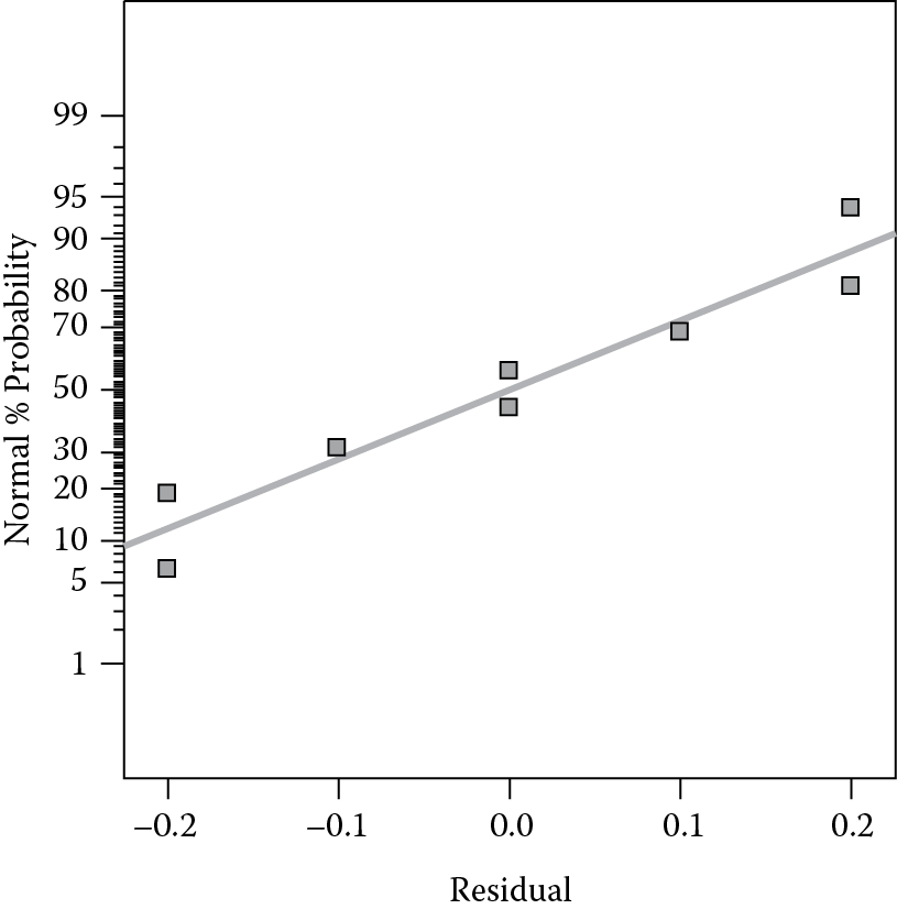
The residuals (Resid), calculated from the difference of actual versus predicted response, can be plotted on normal probability paper. The procedure for creating a full-normal plot is the same as that shown earlier for the half-normal plot, but you don’t need to take the absolute value of the data. Just be sure you have the correct variety of graph paper. In this case, we have eight points so, to be evenly dispersed across the range of 100 percent, the cumulative probabilities Pi should be set at these eight intervals: 6.25, 18.75, 31.25, 43.75, 56.25, 68.75, 81.25, and 93.75%. The resulting plot is shown on Figure 3.11.

If the residuals are normally distributed, they will all fall in a line on this special paper. In this case, the deviations from linear are very minor, so it supports the assumption of normality. Watch for clearly nonlinear patterns, such as an “S” shape. Then consider doing a response transformation, a topic that will be discussed in the next section.
Figure 3.12 shows the normal plot of residuals for the second response (bullets). Give it the pencil test. You will find that residuals for the bullets exhibit no major deviations from the normal line.
The other recommended plot for diagnostics is the residuals versus predicted response. Using the data from Table 3.11, we constructed the plot shown in Figure 3.13.

Ideally, the vertical spread of data will be approximately the same from left to right. Watch for a megaphone (<) pattern, where the residuals increase with the predicted level. In a design as small as that used for the popcorn experiment, only 8 runs, it’s hard to detect patterns. However, it’s safe to say that there is no definite increase in residuals with predicted level, which supports the underlying statistical assumption of constant variance. In the next chapter, we will show you what to do if the residuals are not normal and exhibit nonconstant variance.
Figure 3.14 shows the residual versus predicted plot for the second response (bullets). You don’t need to apply the rule of thumb because there is no obvious increase in residuals as the predicted value increases.

Practice Problems
Problem 3.1
Montgomery describes a two-level design on a high-pressure vessel for making waferboard glue (see Recommended Readings: Design and Analysis of Experiments (2012), example 6.2). A full-factorial experiment is carried out in the pilot plant to study four factors thought to influence the filtration rate of the product. Table 3.12 shows actual high and low levels for each of the factors.
Factors and levels for two-level factorial design on a reactor
|
Factor |
Name |
Units |
Low Level (−) |
High Level (+) |
|
A |
Temperature |
Deg C |
24 |
35 |
|
B |
Pressure |
Psig |
10 |
15 |
|
C |
Concentration |
Percent |
2 |
4 |
|
D |
Stir Rate |
RPM |
15 |
30 |
At each combination of these machine settings, the experimenters recorded the filtration rate. The goal is to maximize the filtration rate and also try to find conditions that would allow a reduction in the concentration of formaldehyde, factor C.
The response data are tabulated in standard order, with factor levels coded, in Table 3.13.
Design layout and response data for reactor study
|
Standard |
A |
B |
C |
D |
Filtration Rate (gallons per hour) |
|
1 |
– |
– |
– |
– |
45.0 |
|
2 |
+ |
– |
– |
– |
71.0 |
|
3 |
– |
+ |
– |
– |
48.0 |
|
4 |
+ |
+ |
– |
– |
65.0 |
|
5 |
– |
– |
+ |
– |
68.0 |
|
6 |
+ |
– |
+ |
– |
60.0 |
|
7 |
– |
+ |
+ |
– |
80.0 |
|
8 |
+ |
+ |
+ |
– |
65.0 |
|
9 |
– |
– |
– |
+ |
43.0 |
|
10 |
+ |
– |
– |
+ |
100.0 |
|
11 |
– |
+ |
– |
+ |
45.0 |
|
12 |
+ |
+ |
– |
+ |
104.0 |
|
13 |
– |
– |
+ |
+ |
75.0 |
|
14 |
+ |
– |
+ |
+ |
86.0 |
|
15 |
– |
+ |
+ |
+ |
70.0 |
|
16 |
+ |
+ |
+ |
+ |
96.0 |
Do an analysis of the data to see if any effects are significant. Recommend operating conditions that maximize rate with a minimum of formaldehyde. (Suggestion: Use the software provided with the book. First do the two-level factorial tutorial that comes with the program. It’s keyed to the data in Table 3.13. See About the Software for software installation instructions and details on the associated tutorials.)
Problem 3.2
Modern cars are built with such precision that they become hermetically sealed when locked. As a result, the interior becomes unbearably hot in cars parked outdoors on warm, sunny days. A variety of window covers can be purchased to alleviate the heat. The materials vary, but generally the covers present either a white or shiny, metallic surface that reflects solar radiation. In some cases, they can be flipped to one side or the other. The white variety of cover usually displays some sort of printed pattern, such as a smiling sun or the logo of a local sports team. These patterns look good, but they may detract from the heat-shielding effect. A two-level factorial design was conducted to quantify the effects of several potential variables: cover (shiny versus white), direction of the parked car (east versus west), and location (near the office in an open lot versus far away from the office under a shade tree).
The resulting 8-run, two-level DOE was performed during a period of stable weather in Minneapolis during early September. Anticipating possible variations, the experimenter (Mark) recorded temperature, cloudiness, wind speed, and other ambient conditions. Outside temperatures ranged from 66 to 76°F under generally clear skies. Randomization of the run order provided insurance against the minor variations in weather. The response shown in Table 3.14 is the difference in temperature from inside to outside as measured by a digital thermometer.
Results from car-shade experiment
|
Std |
A: Cover |
B: Orientation |
C: Location |
Temp Increase (°F) |
|
1 |
White |
East |
Close/Open |
42.1 |
|
2 |
Shiny |
East |
Close/Open |
20.8 |
|
3 |
White |
West |
Close/Open |
54.3 |
|
4 |
Shiny |
West |
Close/Open |
23.2 |
|
5 |
White |
East |
Far/Shaded |
17.4 |
|
6 |
Shiny |
East |
Far/Shaded |
10.4 |
|
7 |
White |
West |
Far/Shaded |
11.7 |
|
8 |
Shiny |
West |
Far/Shaded |
16.0 |
Even in this relatively mild late-summer season, the inside temperatures of the automobile often exceeded 100°F. It’s not hard to imagine how hot it could get under extreme midsummer weather. Analyze this data to see what, if any, factors prove to be significant. Make a recommendation on how to shade the car and how and where to park it. (Suggestion: Use the software provided with the book. Set up a factorial design, similar to the one you did for the tutorial that comes with the program, for three factors in eight runs. Sort the design by standard order to match the table above and enter the data. Then do the analysis as outlined in the tutorial.)
Appendix: How to Make a More Useful Pareto Chart
The Pareto chart is useful for showing the relative size of effects, especially to nonstatisticians. However, if a two-level factorial design gets botched, for example, due to a breakdown during one particular run, it becomes unbalanced and nonorthogonal, thus causing the effects to exhibit differing standard errors. In such cases, the absolute magnitude of an effect may not reflect its statistical significance. To make the Pareto chart more robust to experimental mishaps, we recommend it be plotted with the t-values of the effects. Furthermore, in this dimensionless statistical scale, it becomes appropriate to superimpose benchmarks for significance as detailed in this appendix, which follows up on the less-sophisticated Pareto chart laid out earlier for the effects on popcorn bullets (unpopped kernels).
The t-value is computed by simply dividing the numerical effect by its associated standard error, which is easy to calculate for a balanced, orthogonal experiment like that done on microwave popcorn. Below is the formula in this special case:
where n represents the number of responses from each of the two levels tested and MS is the mean square for the residuals computed by the ANOVA. For the largest effect on the weight of popcorn bullets—C (seen at the bottom of Table 3.7)—the t-value is calculated as follows:
Similar calculations can be performed to obtain t-values for the other six effects, which can then be bar-charted in descending order. However, before doing this, it will be very helpful to look up the two-tailed t-value for 0.05 probability (or some other p-value that you establish depending on your threshold for risk) from the table in Appendix 1.1. The degrees of freedom (df) can be read off the ANOVA for the residuals. In this case, the df are 4 (from Table 3.10), so the critical t-value is 2.776. A more conservative t-value, named after its inventor (Bonferroni), takes the number of estimated effects into account by dividing it into the desired probability for the risk value alpha (α). For the popcorn experiment, seven effects are estimated, so the Bonferroni-corrected p-value becomes:
This value can be calculated precisely by statistical software, but approximated values from a table (such as the one in Appendix 1) may suffice for seeing which effects, if any, stand out from those caused by chance variation.
The Pareto chart in terms of t-values with the two threshold limits is shown in Figure 3.15.

All three labeled effects (C, B, and BC) exceed even the more conservative Bonferroni limit, thus providing a high level of confidence; greater than 95%.
Hay!
Perhaps the earliest known multifactor experiment of this kind was laid out in 1898 by agronomists from Newcastle University in the United Kingdom, who varied the amounts of nitrogen (N), potash (K), and phosphate (K) via a two-level factorial design on Palace Leas meadow. In this field (last ploughed during the Napoleonic Wars), they applied the eight combinations of N, P, and K into individual plots. The results led to an impressive increase in crop yields. (Source: Shirley Coleman, et. al. 1987. The effect of weather and nutrition on the yield of hay from Palace Leas meadow hay plots, at Cockle Park Experimental Farm, over the period from 1897 to 1980. Grass and Forage Science 42: 353–358.)
Be Aggressive in Setting Factor Levels, But Don’t Burn the Popcorn
One of the most difficult decisions for design of experiments (DOE), aside from which factors to choose, is what levels to set them. A general rule is to set levels as far apart as possible so you will more likely see an effect, but not exceed the operating boundaries. For example, test pilots try to push their aircraft to the limits, a process often called pushing the envelope. The trick is not to break the envelope, because the outcome may be “crash and burn.” In the actual experiment on popcorn (upon which the text example is loosely based), the experiment designer (Mark) set the upper level of time too high. In the randomized test plan, several other combinations were run successfully before a combination of high time and high power caused the popcorn to erupt like a miniature volcano, emitting a lava-hot plasma of butter, steam, and smoke. Alerted by the kitchen smoke alarm, the family gathered to observe the smoldering microwave oven. Mark was heartened to hear the children telling his wife not to worry because “in science, you learn from your mistakes.” Her reaction was not as positive, but a new microwave restored harmony to the household. Lessen learned—always conduct highly controlled pretrials on extreme combinations of factors!
Always Randomize Your Run Order
You must randomize the order of your experimental runs to satisfy the statistical requirement of independence of observations. Randomization acts as insurance against the effects of lurking time-related variables, such as the warm-up effect on a microwave oven. For example, let’s say you forget to randomize and first run all low levels of a factor and then all high levels of a given factor that actually creates no effect on response. Meanwhile, an uncontrolled variable causes the response to gradually increase. In this case, you will mistakenly attribute the happenstance effect to the nonrandomized factor. By randomizing the order of experimentation, you greatly reduce the chances of such a mistake. Select your run numbers from a table of random numbers or mark them on slips of paper and simply pull them blindly from a container. Statistical software can also be used to generate random run orders.
“Designing an experiment is like gambling with the devil: only a random strategy can defeat all his betting systems.”
Sir Ronald Fisher
Orthogonal Arrays: When You Have Limited Resources, It Pays to Plan Ahead
The standard two-level factorial layout shown in Table 3.3 is one example of a carefully balanced “orthogonal array.” Technically, this means that there is no correlation among the factors. You can see this most easily by looking at column C. When C is at the minus level, factors A and B contain an equal number of pluses and minuses, thus, their effect cancels. The same result occurs when C is at the plus level. Therefore, the effect of C is not influenced by factors A or B. The same can be said for the effects of A and B and all the interactions as well. The authors have limited this discussion of orthogonal arrays to those that are commonly called the standard arrays for two-level full and fractional factorials. However, you may come across other varieties of orthogonal arrays, such as Taguchi and Plackett-Burman. Note, however, that any orthogonal test array is much preferred to unplanned experimentation (an oxymoron). Happenstance data are likely to be highly correlated (nonorthogonal), which makes it much more difficult to sort out the factors that really affect your response. (For an in-depth explanation of the dangers in dealing with nonorthogonal matrices, see Chapter 2, Lessons to Learn from Happenstance Regression, in RSM Simplified.)
The Vital Few versus the Trivial Many
A rule of thumb, called sparsity of effects, says that, in most systems, only 20% of the main effects (MEs) and two-factor interactions (2 fi) will be significant. The other ME and 2 fis, as well as any three-factor interactions (3 fi) or greater will vary only to the extent of normal error. (Remember that the effects are based on averages, so their variance will be reduced by a factor of n.) This rule of thumb is very similar to that developed a century ago by economist Vilfredo Pareto, who found that 80% of the wealth was held by 20% of the people. Dr. Joseph Juran, a preeminent figure in the twentieth-century quality movement, applied this 80/20 rule to management: 80% of the trouble comes from 20% of the problems. He advised focusing effort on these “vital few” problems and ignoring the “trivial many.”
Taste Is in the Mouth of the Beholder
Before being rescaled, the popcorn taste was rated on a scale of 1 (worst) to 10 (best) by a panel of Minnesotans. The benchmarks they used reflect a conservative, Scandinavian heritage:
10: Just like lutefisk*
9: Not bad for you
8: Tastes like Mom’s
7: Not so bad
6: Could be better
5: Could be worse
4: My spouse made something like this once
3: I like it, but …
2: It’s different
1: Complete silence
If you are not from Minnesota, we advise that you use an alternative scale used by many sensory evaluators, which goes from 1 to 9, with 9 being the best. All nine numbers are laid out in line. The evaluator circles the number that reflects his or her rating of a particular attribute. To avoid confusion about orientation of the scale, we advise that you place sad (![]() ), neutral (
), neutral (![]() ), and happy (
), and happy (![]() ) faces at the 1, 5, and 9 positions on the number line, respectively. This is called a “hedonic” scale. Rating scales like this can provide valuable information on subjective responses, particularly when you apply the averaging power of a well-planned experiment.
) faces at the 1, 5, and 9 positions on the number line, respectively. This is called a “hedonic” scale. Rating scales like this can provide valuable information on subjective responses, particularly when you apply the averaging power of a well-planned experiment.
* Dried cod soaked in lye that is rumored to be good for removing wallpaper—just throw the fish up by the ceiling and let it slide all the way down for broadest application.
How SS Simplifies: A Quick Explanation
(Try following along with this text only if you really care where the sum of squares formula came from.) The difference from either the plus or minus results to the overall experimental response average (also known as the somewhat pompous grand mean) is equal to one-half of the effect. (See Figure 3.10 for illustration.) Half of the runs are plus and half are minus. Thus:
SS = SSplus + SSminus = N/2(Effect/2)2 + N/2(Effect/2)2 = 2 (N/2(Effect/2)2
= N/4(Effect)2
So now you know.
Why Popcorn Pops (or Doesn’t)
Before designing any experiment, it pays to gather knowledge about the subject matter so you can more intelligently choose factors. This studious approach also provides perspective for assessing the apparent effects that emerge from the statistical analysis. For example, here is some subject matter background that may “a-maize” you. Corn used for popping comes from a special strain called pericarp, characterized by an outer covering that is stronger and more airtight than that of other corn varieties. Like all corn, pericarp contains moisture, which when heated, becomes superheated steam. At some point, the pressure causes an explosive rupture in the coating of the popcorn. The white ball of well-popped corn is made up of mostly protein and starch granules that expand to 30 times in volume when popped. Unpopped kernels may be caused by seemingly slight scratches in the coating that allow the heated moisture to gradually escape, rather than build up. Too little moisture in the kernels may also cause problems with popping. On the other hand, excessive moisture results in tough, rather than crunchy, popcorn.
The Pencil Test
Recall from Chapter 1 that a simple, but effective, way to check for linearity is to place a pencil on the normal probability graph. If the pencil covers all the points, consider it in line. A large marker pen would solve all your problems!
A Literal Rule of Thumb
ANOVA and other statistical analyses are relatively robust to deviations from normality and constancy of variance. Therefore, you should not overreact to slight nonlinearity on the normal plot of residuals, or to vague patterns on the residuals versus predicted plot. As a rule of thumb, if you think you see a pattern, but it disappears when you cover one point with your thumb, then don’t worry. However, if you have a touch screen computer, do not get carried away with this procedure.
P.S.: Despite rumors to the contrary, the term rule of thumb probably came from use of the thumb as a crude measure of length. However, it may refer to the traditional practice of brewmasters who check temperature of beer by dipping their thumbs in the batch. This latter explanation is most consistent with the origins of the t-test and other statistical innovations.
For Those Consumers Who May Not Be Firing on All Cylinders
Operating instructions seen on accordion-style, front-window shade for automobiles: “Remove before driving.”
Another Italian Mathematician: Bonferroni
Carlo Emilio Bonferroni (1892–1960) joined his predecessor Pareto in the pantheon of Italian mathematicians that include such luminaries as Fibonacci. Bonferroni’s famous Correction states that if an experimenter tests n independent hypotheses, then the statistical significance level should be n times smaller than usual. For example, when testing two hypotheses, instead of assigning a p-value of 0.05, one should cut this value in half, to a much stricter level of 0.025. The Bonferroni Correction safeguards against multiple tests of statistical significance on the same data.
For example, when the authors worked for General Mills, the head of quality control in Minneapolis would mix up a barrel of flour and split it into 10 samples, carefully sealed in air-tight containers, for each of the mills to test in triplicate for moisture. A naïve analyst would have simply taken the highest moisture value and compared it to the lowest one. But given that there are 45 possible pair-wise comparisons (10*9/2), this selection (high versus low) is likely to produce a result that tests significant at the 0.05 level (1 out of 20). Refer to the 6/6/10 StatsMadeEasy blog “Bonferroni of Bergamo” (www.statsmadeeasy.net/ 2010/06/bonferroni-of-bergamo/) for the results of a simulation that graphically demonstrates the bias, if uncorrected, introduced by such a multiple pair-wise comparison.
“I do not feel obliged to believe that the same God who has endowed us with sense, reason, and intellect has intended us to forgo their use.”
Galileo Galilei