ETL and ELT

There is perhaps no pattern more well known that ETL (Extract, Transform, Load) and it’s more modern sibling, ELT (Extract, Load, Transform). Both are patterns widely used in data warehousing and business intelligence. In more recent years, they’ve inspired pipeline patterns for data science and machine learning models running in production. They are so well known in fact, that many people use these terms synonymously with data pipelines rather than patterns that many pipelines follow.

Given their roots in data warehousing, it’s easiest to describe them in that context, which I do in this section. Later sections in this chapter describe how they are used for particular use cases.

Both patterns are approaches to data processing used to feed data into a data warehouse and make it useful to analysts and reporting tools. The difference between the two is the order of their final two steps (Transform and Load), but the design implications in choosing between them are substantial as I’ll explain throughout this chapter. First, let’s explore the steps of ETL and ELT.

The Extract step is gathers data from various sources in preparation for loading and transforming. Chapter 2 discussed the diversity of these sources and methods of extraction.

The Load step either brings in the raw data (in the case of ELT) or the fully transformed data (in the case of ETL) into the final destination. Either way, the end result is loading data into the data warehouse, data lake or other destination.

The Transform step is where the raw data from each source system is combined and formatted in a such a way that it’s useful to analysts, visualization tools, or whatever use case your pipeline is serving. There’s a lot to this step regardless of whether you design your process as ETL or ELT, all of which is explored in detail in Chapter 5.

The Emergence of ELT over ETL

ETL was the gold standard of data pipeline patterns for decades. Though it’s still used, more recently ELT has emerged as the pattern of choice. Why? Prior to the modern breed of data warehouses, primarily in the cloud (see Chapter 2), data teams didn’t have access to data warehouses with the storage or compute necessary to handle loading vast amounts of raw data and transforming into useable data models all in the same place. In addition, data warehouses at the time were row based databases that worked well for transactional use cases, but not for the high volume, bulk queries that are commonplace in analytics. Thus, data was first extracted from source systems and then transformed on a separate system before being loaded into a warehouse for any final data modeling and querying by analysts and visualization tools.

The majority of today’s data warehouses are built on highly scalable, columnar databases that can both sore and run bulk transforms on large datasets in a cost effective manner. Thanks to the I/O efficiency of a columnar database, data compression, and the ability to distribute data and queries across many nodes that can work together to process data things have changed. It’s now better to focus on extracting data and loading it into a data warehouse where you can then perform the necessary transformations to complete the pipeline.

The impact of the difference between row and column based data warehouses cannot be overstated. Figure 3.1 below illustrates an example of how records are stored on disk in a row based database. Each row of the database is stored together on disk, in one or more blocks depending on the size of each record. If a record is smaller than a single block, or not cleanly divisible by the block size, it leaves some disk space unused.

Figure 3-1. A table stored in a row-based storage database. Each block contains a record (row) from the table.

Consider an OLTP (online transaction processing) database use case such as an e-commerce web application that leverages a MySQL database for storage. The web app requests reads and writes from and to the MySQL database, often involving multiple values from each record such as the details of an order on an order confirmation page. It’s also likely only to query or update one order at a time. Therefore, row-based stored is optimal since the data the application needs is stored in close proximity on disk, and he amount of data queried at one time is small.

The inefficient use of disk space due to records leaving empty space in blocks is a reasonable trade-off in this case, as the speed to reading and writing single records frequently is what’s most important. However, in analytics the situation is reversed. Instead of the need to read and write small amounts of data frequently, we often read and write large amount of data infrequently. In addition, it’s less likely that an analytical query requires many, or all, of the columns in a table but rather a single column of a table with many columns.

For example, consider the order table in our fictional e-commerce application. Among other things, it contains the dollar amount of the order as well as the country it’s shipping to. Unlike the web application which works with orders one at a time, an analyst using the data warehouse will want to analyze orders in bulk. In addition, the table containing order data in the data warehouse has additional columns that contain values from multiple tables in our MySQL database. For example, it might contain the information about the customer that placed the order. Perhaps the analyst wants to sum up all orders placed but customers with currently active accounts. Such a query might involve millions of records, but only read from two columns, OrderTotal and CustomerActive.

As illustrated in figure 3.2, a columnar database stores data in disk blocks by column rather than row. In our use case, the query written by the analyst only needs to access blocks that store OrderTotal and CustomerActive values rather than blocks that store the row based records such as the MySQL database. Thus, there’s less disk I/O as well as less data to load into memory to perform the filtering and summing required by the analysts query. A final benefit is reduction in storage thanks to the fact that blocks can be fully utilized and optimally compressed since the same datatype is stored in each block rather than multiple types that tend to occur in a single row-based record.

Figure 3-2. A table stored in a column-based storage database. Each disk block contains data from the same column. The two columns involved in our example query are highlighted. Only these blocks must be accessed to run the query. Each block contains data of the same type, making compression optimal.

All in all, the emergence of columnar databases means that storing, transforming, and querying large datasets is efficient within a data warehouse. Data engineers can use that to their advantage by building pipeline steps that specialize in extracting and loading data into warehouses where it can be transformed, modeled and queried by analysts and data scientists who are more comfortable within the confines of a database. As such, ELT has taken over as the ideal pattern for data warehouse pipelines as well as other use cases in machine learning and data product development.

EtLT Subpattern

When ELT emerged as the dominant pattern, it became clear that doing some transformation after extraction, but before loading was still beneficial. However, instead of transformation involving business logic or data modeling this type of transformation is more limited in scope. I refer to this as “lowercase t” transformation, hence EtLT.

Some examples of the type of transformation that fits into the EtLT sub-pattern include the following.

• Deduplicate records in a table

• Parse URL parameters into individual components

• Mask or otherwise obfuscate sensitive data

These types of transforms are either fully disconnected from business logic, or in the case of something like masking sensitive data, at times required as early in a pipeline as possible for legal or security reasons. In addition, there is value in using the right tool for the right job. As Chapter 4 illustrates in greater detail, most modern data warehouses load data most efficiently if it’s prepared well. In pipelines moving a high volume of data, or where latency is key, performing some basic transforms between the Extract and Load steps is worth the effort.

In the remaining ELT-related patterns, it can be assumed that they are designed to include the EtLT sub-pattern as well.

ELT for Data Analysis

ELT has become the most common, and in my opinion, most optimal pattern for pipelines built for data analysis. As already discussed, columnar databases are well suited to handling high volumes of data. They are also designed to handle wide tables, meaning tables with many columns, thanks to the fact that only data in columns used in a given query are scanned on disk and loaded into memory.

Beyond technical considerations, data analysts are typically fluent in SQL. With ELT, data engineers can focus on the extract and load steps in a pipeline (data ingestion) while analysts can utilize SQL to transform the data that’s been ingested as needed for reporting and analysis. Such a clean separation is not possible with an ETL pattern, as data engineers are needed across the entire pipeline. As shown in Figure 3.3, ELT allows data team members to focus on their strengths with less interdependencies and coordination.

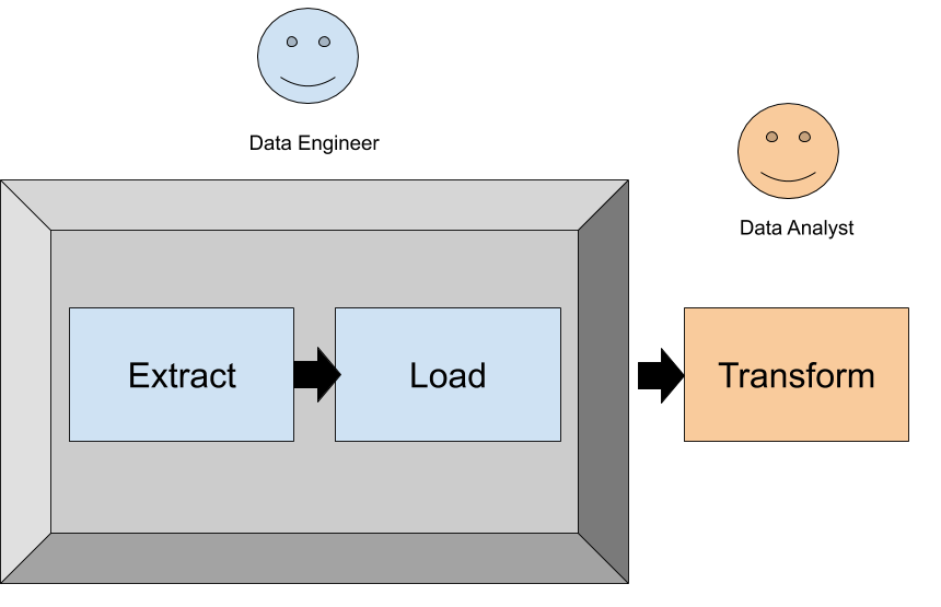
Figure 3-3. The ELT pattern allows for a clean split of responsibilities between data engineers and data analysts (or data scientists). Each role can work autonomously with the tools and language they are comfortable in.

ELT for Data Science

Data pipelines built for data science teams are very similar to those built for data analysis in a data warehouse. Like the analysis use case, data engineers are focused on ingesting data into a data warehouse or data lake. However, data scientists have different needs from the data than data analysts do.

Though data science is a broad field, in general data scientists will need access to more granular, and at times raw, data than data analysts do. While data analysts build data models that produce metrics and power dashboards, data scientists spend their days exploring data and building predictive models. While the details of the role of a data scientist are out of the scope of this book, this high level distinction matters to the design of pipelines serving data scientists.

ELT for Data Products

Data is used for more than analysis, reporting and predictive models. It’s also used for powering data products. Some common examples of data products include the following.

• A content recommendation engine that powers a video streaming home screen

• A personalized search engine on an e-commerce website

• An application that performs sentiment analysis on user generated restaurant reviews

Each of those data products are likely powered by one or more machine learning models, which are hungry for training and validation data. Such data may come from a variety of source systems and undergo some level of transformation to prepare it for use in the model. An ELT pattern is well suited for such needs, though there are a number of specific challenges in all steps of a pipeline that’s designed for a data product. Chapter 6 is focused on machine learning focused data pipelines.