2
Introducing Dask
- Warming up with a short example of data cleaning using Dask DataFrames
- Visualizing DAGs generated by Dask workloads with graphviz
- Exploring how the Dask task scheduler applies the concept of DAGs to coordinate execution of code
Now that you have a basic understanding of how DAGs work, let’s take a look at how Dask uses DAGs to create robust, scalable workloads. To do this, we’ll use the NYC Parking Ticket data you downloaded at the end of the previous chapter. This will help us accomplish two things at once: you’ll get your first taste of using Dask’s DataFrame API to analyze a structured dataset, and you’ll start to get familiar with some of the quirks in the dataset that we’ll address throughout the next few chapters. We’ll also take a look at a few useful diagnostic tools and use the low-level Delayed API to create a simple custom task graph.
Before we dive into the Dask code, if you haven’t already done so, check out the appendix for instructions on how to install Dask and all the packages you’ll need for the code examples in the remainder of the book. You can also find the complete code notebooks online at www.manning.com/books/data-science-with-python-and-dask and also at http://bit.ly/daskbook. For all the examples throughout the book (unless otherwise noted), I recommend you use a Jupyter Notebook. Jupyter Notebooks will help you keep your code organized and will make it easy to produce visualizations when necessary. The code in the examples has been tested in both Python 2.7 and Python 3.6 environments, so you should be able to use either without issue. Dask is available for both major versions of Python, but I highly recommend that you use Python 3 for any new projects, because the end of support for Python 2 is slated for 2020.
Finally, before we get going, we’ll take a moment to set the table for where we’ll be headed over the next few chapters. As mentioned before, the objective of this book is to teach you the fundamentals of Dask in a pragmatic way that focuses on how to use it for common data science tasks. Figure 2.1 represents a fairly standard way of approaching data science problems, and we’ll use this workflow as a backdrop to demonstrate how to apply Dask to each part of it.
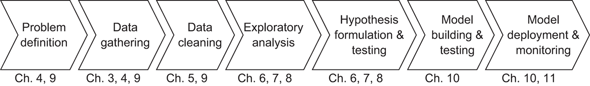
Figure 2.1 Our workflow, at a glance, in Data Science with Python and Dask
In this chapter, we’ll take a look at a few snippets of Dask code that fall into the areas of data gathering, data cleaning, and exploratory analysis. However, chapters 4, 5, and 6 will cover those topics much more in depth. Instead, the focus here is to give you a first glimpse of what Dask syntax looks like. We’ll also focus on how the high-level commands we give Dask relate to the DAGs generated by the underlying scheduler. So, let’s get going!
2.1 Hello Dask: A first look at the DataFrame API
An essential step of any data science project is to perform exploratory analysis on the dataset. During exploratory analysis, you’ll want to check the data for missing values, outliers, and any other data quality issues. Cleaning the dataset ensures that the analysis you do, and any conclusions you make about the data, are not influenced by erroneous or anomalous data. In our first look at using Dask DataFrames, we’ll step through reading in a data file, scanning the data for missing values, and dropping columns that either are missing too much data or won’t be useful for analysis.
2.1.1 Examining the metadata of Dask objects
For this example, we’ll look at just the data collected from 2017. First, you’ll need to import the Dask modules and read in your data.
Listing 2.1 Importing relevant libraries and data
import dask.dataframe as dd
from dask.diagnostics import ProgressBar
from matplotlib import pyplot as plt    ①
df = dd.read_csv('nyc-parking-tickets/*2017.csv')    ②
df
If you’re an experienced Pandas user, listing 2.1 will look very familiar. In fact, it is syntactically equivalent! For simplicity’s sake, I’ve unzipped the data into the same folder as the Python notebook I’m working in. If you put your data elsewhere, you will either need to find the correct path to use or change your working directory to the folder that contains your data using os.chdir. Inspecting the DataFrame we just created yields the output shown in figure 2.2.
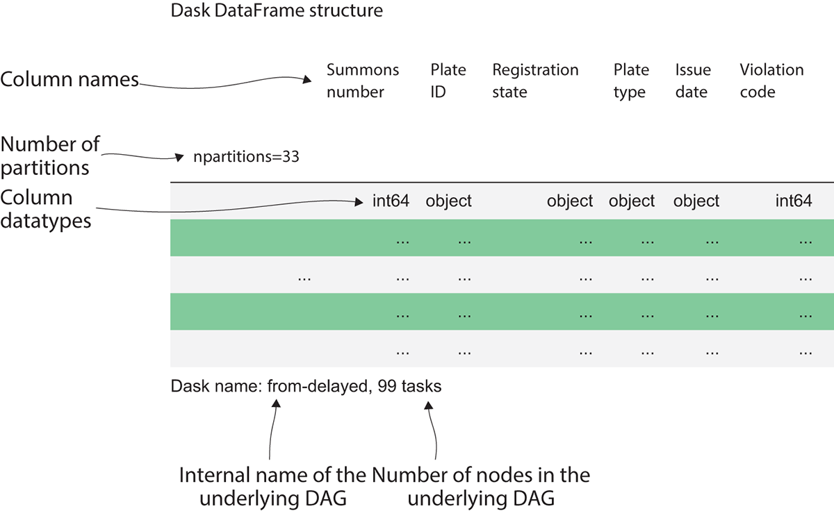
Figure 2.2 Inspecting the Dask DataFrame
The output of listing 2.1 might not be what you expected. While Pandas would display a sample of the data, when inspecting a Dask DataFrame, we are shown the metadata of the DataFrame. The column names are along the top, and underneath is each column’s respective datatype. Dask tries very hard to intelligently infer datatypes from the data, just as Pandas does. But its ability to do so accurately is limited by the fact that Dask was built to handle medium and large datasets that can’t be loaded into RAM at once. Since Pandas can perform operations entirely in memory, it can quickly and easily scan the entire DataFrame to find the best datatype for each column. Dask, on the other hand, must be able to work just as well with local datasets and large datasets that could be scattered across multiple physical machines in a distributed filesystem. Therefore, Dask DataFrames employ random sampling methods to profile and infer datatypes from a small sample of the data. This works fine if data anomalies, such as letters appearing in a numeric column, are widespread. However, if there’s a single anomalous row among millions or billions of rows, it’s very improbable that the anomalous row would be picked in a random sample. This will lead to Dask picking an incompatible datatype, which will cause errors later on when performing computations. Therefore, a best practice to avoid that situation would be to explicitly set datatypes rather than relying on Dask’s inference process. Even better, storing data in a binary file format that supports explicit data types, such as Parquet, will avoid the issue altogether and bring some additional performance gains to the table as well. We will return to this issue in a later chapter, but for now we will let Dask infer datatypes.
The other interesting pieces of information about the DataFrame’s metadata give us insight into how Dask’s scheduler is deciding to break up the work of processing this file. The npartitions value shows how many partitions the DataFrame is split into. Since the 2017 file is slightly over 2 GB in size, at 33 partitions, each partition is roughly 64 MB in size. That means that instead of loading the entire file into RAM all at once, each Dask worker thread will work on processing the file one 64 MB chunk at a time.
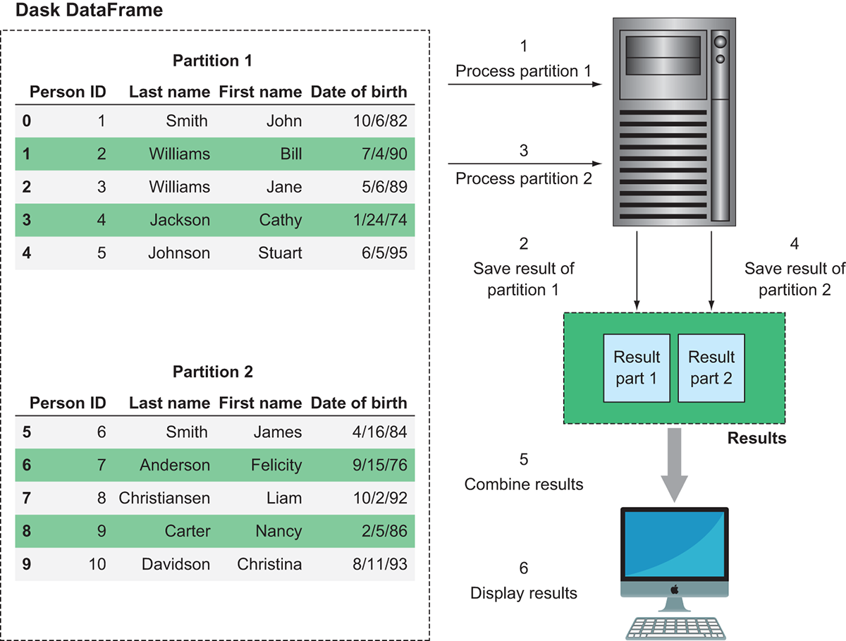
Figure 2.3 Dask splits large data files into multiple partitions and works on one partition at a time.
Figure 2.3 demonstrates this behavior. Rather than eagerly loading the entire DataFrame into RAM, Dask breaks the file into smaller chunks that can be worked on independently. These chunks are called partitions. In the case of Dask DataFrames, each partition is a relatively small Pandas DataFrame. In the example in figure 2.3, the DataFrame consists of two partitions. Therefore, the single Dask DataFrame is made up of two smaller Pandas DataFrames. Each partition can be loaded into memory and worked on one at a time or in parallel. In this case, the worker node first picks up partition 1 and processes it, and saves the result in a temporary holding space. Next it picks up partition 2 and processes it, saving the result to a temporary holding space. Finally, it combines the results and ships it down to our client, which displays the result. Because the worker node can work on smaller pieces of the data at a time, work can be distributed out to many machines. Or, in the case of a local cluster, work can proceed on very large datasets without resulting in out-of-memory errors.
The last bit of metadata we got from our DataFrame is that it consists of 99 tasks. That’s telling us that Dask created a DAG with 99 nodes to process the data. The graph consists of 99 nodes because each partition requires three operations to be created: reading the raw data, splitting the data into the appropriately sized block, and initializing the underlying DataFrame object. In total, 33 partitions with 3 tasks per partition results in 99 tasks. If we had 33 workers in our worker pool, the entire file could be worked on simultaneously. With just one worker, Dask will cycle through each partition one at a time. Now, let’s try to count the missing values in each column across the entire file.
Listing 2.2 Counting missing values in the DataFrame
missing_values = df.isnull().sum()
missing_values

Dask Series Structure:
npartitions=1
Date First Observed    int64
Violation Time           ...
dtype: int64
Dask Name: DataFrame-sum-agg, 166 tasks
The syntax for counting null values again looks a lot like Pandas. But as before, inspecting the resulting Series object doesn’t give us the output we might expect. Instead of getting the missing counts, Dask returns some metadata information about the expected result. It looks like missing_values is a Series of int64s, but where’s the actual data? Dask hasn’t actually done any processing yet because it uses lazy computation. This means that what Dask has actually done under the hood is prepare another DAG, which was then stored in the missing_values variable. The data isn’t computed until the task graph is explicitly executed. This behavior makes it possible to build up complex task graphs quickly without having to wait for each intermediate step to finish. You might notice that the tasks count has grown to 166 now. That’s because Dask has taken the first 99 tasks from the DAG used to read in the data file and create the DataFrame called df, added 66 tasks (2 per partition) to check for nulls and sum, and then added a final step to collect all the pieces together into a single Series object and return the answer.
Listing 2.3 Calculating the percent of missing values in the DataFrame
missing_count = ((missing_values / df.index.size) * 100)
missing_count

Dask Series Structure:
npartitions=1
Date First Observed    float64
Violation Time             ...
dtype: float64
Dask Name: mul, 235 tasks
Before we run the computation, we’ll ask Dask to transform these numbers into percentages by dividing the missing value counts (missing_values) by the total number of rows in the DataFrame (df.index.size), then multiplying everything by 100. Notice that the number of tasks has increased again, and the datatype of the resulting Series changed from int64 to float64! This is because the division operation resulted in answers that were not whole (integer) numbers. Therefore, Dask automatically converted the answer to floating-point (decimal) numbers. Just as Dask tries to infer datatypes from files, it will also try to infer how operations will affect the datatype of the output. Since we’ve added a stage to the DAG that divides two numbers, Dask infers that we’ll likely move from integers to floating-point numbers and changes the metadata of the result accordingly.
2.1.2 Running computations with the compute method
Now we’re ready to run and produce our output.
Listing 2.4 Computing the DAG
with ProgressBar():
   missing_count_pct = missing_count.compute()
missing_count_pct

Summons Number                         0.000000
Plate ID                               0.006739
Registration State                     0.000000
Plate Type                             0.000000
Issue Date                             0.000000
Violation Code                         0.000000
Vehicle Body Type                      0.395361
Vehicle Make                           0.676199
Issuing Agency                         0.000000
Street Code1                           0.000000
Street Code2                           0.000000
Street Code3                           0.000000
Vehicle Expiration Date                0.000000
Violation Location                    19.183510
Violation Precinct                     0.000000
Issuer Precinct                        0.000000
Issuer Code                            0.000000
Issuer Command                        19.093212
Issuer Squad                          19.101506
Violation Time                         0.000583
Time First Observed                   92.217488
Violation County                       0.366073
Violation In Front Of Or Opposite     20.005826
House Number                          21.184968
Street Name                            0.037110
Intersecting Street                   68.827675
Date First Observed                    0.000000
Law Section                            0.000000
Sub Division                           0.007155
Violation Legal Code                  80.906214
Days Parking In Effect                25.107923
From Hours In Effect                  50.457575
To Hours In Effect                    50.457548
Vehicle Color                          1.410179
Unregistered Vehicle?                 89.562223
Vehicle Year                           0.000000
Meter Number                          83.472476
Feet From Curb                         0.000000
Violation Post Code                   29.530489
Violation Description                 10.436611
No Standing or Stopping Violation    100.000000
Hydrant Violation                    100.000000
Double Parking Violation             100.000000
dtype: float64
Whenever you want Dask to compute the result of your work, you need to call the .compute() method of the DataFrame. This tells Dask to go ahead and run the computation and display the results. You may sometimes see this referred to as materializing results, because the DAG that Dask creates to run the computation is a logical representation of the results, but the actual results aren’t calculated (that is, materialized) until you explicitly compute them. You’ll also notice that we wrapped the call to compute within a ProgressBar context. This is one of several diagnostic contexts that Dask provides to help you keep track of running tasks, and especially comes in handy when using the local task scheduler. The ProgressBar context will simply print out a text-based progress bar showing you the estimated percent complete and the elapsed time for the computation.
By the output of our missing-values calculation, it looks like we can immediately throw out a few columns: No Standing or Stopping Violation, Hydrant Violation, and Double Parking Violation are completely empty, so there’s no value in keeping them around. We’ll drop any column that’s missing more than 60% of its values (note: 60% is just an arbitrary value chosen for the sake of example; the threshold you use to throw out columns with missing data depends on the problem you’re trying to solve, and usually relies on your best judgement).
Listing 2.5 Filtering sparse columns
columns_to_drop = missing_count_pct[missing_count_pct > 60].index
with ProgressBar():
    df_dropped = df.drop(columns_to_drop, axis=1).persist()
This is interesting. Since we materialized the data in listing 2.4, missing_count_pct is a Pandas Series object, but we can use it with the drop method on the Dask DataFrame. We first took the Series we created in listing 2.4 and filtered it to get the columns that have more than 60% missing values. We then got the index of the filtered Series, which is a list of column names. We then used that index to drop columns in the Dask DataFrame with the same name. You can generally mix Pandas objects and Dask objects because each partition of a Dask DataFrame is a Pandas DataFrame. In this case, the Pandas Series object is made available to all threads, so they can use it in their computation. In the case of running on a cluster, the Pandas Series object will be serialized and broadcasted to all worker nodes.
2.1.3 Making complex computations more efficient with persist
Because we’ve decided that we don’t care about the columns we just dropped, it would be inefficient to re-read the columns into memory every time we want to make an additional calculation just to drop them again. We really only care about analyzing the filtered subset of data we just created. Recall that as soon as a node in the active task graph emits results, its intermediate work is discarded in order to minimize memory usage. That means if we want to do something additional with the filtered data (for example, look at the first five rows of the DataFrame), we would have to go to the trouble of re-running the entire chain of transformations again. To avoid repeating the same calculations many times over, Dask allows us to store intermediate results of a computation so they can be reused. Using the persist() method of the Dask DataFrame tells Dask to try to keep as much of the intermediate result in memory as possible. In case Dask needs some of the memory being used by the persisted DataFrame, it will select a number of partitions to drop from memory. These dropped partitions will be recalculated on the fly when needed, and although it may take some time to recalculate the missing partitions, it is still likely to be much faster than recomputing the entire DataFrame. Using persist appropriately can be very useful for speeding up computations if you have a very large and complex DAG that needs to be reused many times.
This concludes our first look at Dask DataFrames. You saw how, in only a few lines of code, we were able to read in a dataset and begin preparing it for exploratory analysis. The beauty of this code is that it works the same regardless of whether you’re running Dask on one machine or thousands of machines, and regardless of whether you’re crunching through a couple gigabytes of data (as we did here) or analyzing petabytes of data. Also, because of the syntactic similarities with Pandas, you can easily transition workloads from Pandas to Dask with a minimum amount of code refactoring (which mostly amounts to adding Dask imports and compute calls). We’ll go much further into our analysis in the coming chapters, but for now we’ll dig a little deeper into how Dask uses DAGs to manage distribution of the tasks that underpin the code we just walked through.
2.2 Visualizing DAGs
So far, you’ve learned how directed acyclic graphs (DAGs) work, and you’ve learned that Dask uses DAGs to orchestrate distributed computations of DataFrames. However, we haven’t yet peeked “under the hood” and seen the actual DAGs that the schedulers create. Dask uses the graphviz library to generate visual representations of the DAGs created by the task scheduler. If you followed the steps in the appendix to install graphviz, you will be able to inspect the DAG backing any Dask Delayed object. You can inspect the DAGs of DataFrames, series, bags, and arrays by calling the visualize() method on the object.
2.2.1 Visualizing a simple DAG using Dask Delayed objects
For this example, we’ll take a step back from the Dask DataFrame objects seen in the previous example to step down a level of abstraction: the Dask Delayed object. The reason we’ll move to Delayed objects is because the DAGs that Dask creates for even simple DataFrame operations can grow quite large and be hard to visualize. Therefore, for convenience, we’ll use Dask Delayed objects for this example so we have better control over composition of the DAG.
Listing 2.6 Creating some simple functions
import dask.delayed as delayed
from dask.diagnostics import ProgressBar

def inc(i):
   return i + 1

def add(x, y):
   return x + y

x = delayed(inc)(1)
y = delayed(inc)(2)
z = delayed(add)(x, y)

z.visualize()
Listing 2.6 begins by importing the packages needed for this example: in this case, the delayed package and the ProgressBar diagnostic we used previously. Next, we define a couple simple Python functions. The first adds one to its given input, and the second adds the two given inputs. The next three lines introduce the delayed constructor. By wrapping delayed around a function, a Dask Delayed representation of the function is produced. Delayed objects are equivalent to a node in a DAG. The arguments of the original function are passed in a second set of parentheses. For example, the object x represents a Delayed evaluation of the inc function, passing in 1 as the value of i. Delayed objects can reference other Delayed objects as well, which can be seen in the definition of the object z. Chaining together these Delayed objects is what ultimately makes up a graph. For the object z to be evaluated, both of the objects x and y must first be evaluated. If x or y has other Delayed dependencies that must be met as part of their evaluation, those dependencies would need to be evaluated first and so forth. This sounds an awful lot like a DAG: evaluating the object z has a well-known chain of dependencies that must be evaluated in a deterministic order, and there is a well-defined start and end point. Indeed, this is a representation of a very simple DAG in code. We can have a look at what that looks like by using the visualize method.
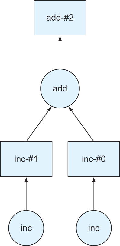
Figure 2.4 A visual representation of the DAG produced in listing 2.6
As you can see in figure 2.4, object z is represented by a DAG. At the bottom of the graph, we can see the two calls to the inc function. That function didn’t have any Delayed dependencies of its own, so there are no lines with arrows pointing into the inc nodes. However, the add node has two lines with arrows pointing into it. This represents the dependency on first calculating x and y before being able to sum the two values. Since each inc node is free of dependencies, a unique worker would be able to work on each task independently. Taking advantage of parallelism like this could be very advantageous if the inc function took a long time to evaluate.
2.2.2 Visualizing more complex DAGs with loops and collections
Let’s look at a slightly more complex example.
Listing 2.7 Performing the add_two operation
def add_two(x):
    return x + 2

def sum_two_numbers(x,y):
    return x + y

def multiply_four(x):
    return x * 4

data = [1, 5, 8, 10]

step1 = [delayed(add_two)(i) for i in data]
total = delayed(sum)(step1)
total.visualize()
Now things are getting interesting. Let’s unpack what happened here. We started again by defining a few simple functions, and also defined a list of integers to use. This time, though, instead of creating a Delayed object from a single function call, the Delayed constructor is placed inside a list comprehension that iterates over the list of numbers. The result is that step1 becomes a list of Delayed objects instead of a list of integers.
The next line of code uses the built-in sum function to add up all the numbers in the list. The sum function normally takes an iterable as an argument, but since it’s been wrapped in a Delayed constructor, it can be passed the list of Delayed objects. As before, this code ultimately represents a graph. Let’s take a look at what the graph looks like.
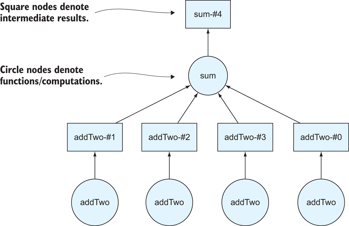
Figure 2.5 The directed acyclic graph representing the computation in listing 2.7
Now, the variable total is a Delayed object, which means we can use the visualize method on it to draw the DAG that Dask will use if we ask Dask to compute the answer! Figure 2.5 shows the output of the visualize method. One thing to notice is that Dask draws DAGs from the bottom up. We started with four numbers in a list called data, which corresponds to four nodes at the bottom of the DAG. The circles on the Dask DAGs represent function calls. This makes sense: we had four numbers, and we wanted to apply the add_two function to each number so we have to call it four times. Similarly, we call the sum function only one time because we’re passing in the complete list. The squares on the DAG represent intermediate results. For instance, the result of iterating over the list of numbers and applying the add_two function to each of the original numbers is four transformed numbers that had two added to them. Just like with the DataFrame in the previous section, Dask doesn’t actually compute the answer until you call the compute method on the total object.
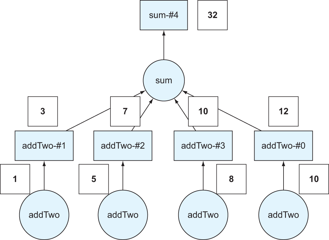
Figure 2.6 The DAG from figure 2.5 with the values superimposed over the computation
In figure 2.6, we’ve taken the four numbers from the data list and superimposed them over the DAG so you can see the result of each function call. The result, 32, is calculated by taking the original four numbers, applying the addTwo transformation to each, then summing the result.
We’ll now add another degree of complexity to the DAG by multiplying every number by four before collecting the result.
Listing 2.8 Multiply each value by four
def add_two(x):
    return x + 2

def sum_two_numbers(x,y):
    return x + y

def multiply_four(x):
    return x * 4

data = [1, 5, 8, 10]

step1 = [delayed(add_two)(i) for i in data]
step2 = [delayed(multiply_four)(j) for j in step1]
total = delayed(sum)(step2)
total.visualize()
This looks an awful lot like the previous code listing, with one key difference. In the first line of code, we apply the multiply_four function to step1, which was the list of Delayed objects we produced by adding two to the original list of numbers. Just like you saw in the DataFrame example, it’s possible to chain together computations without immediately calculating the intermediate results.
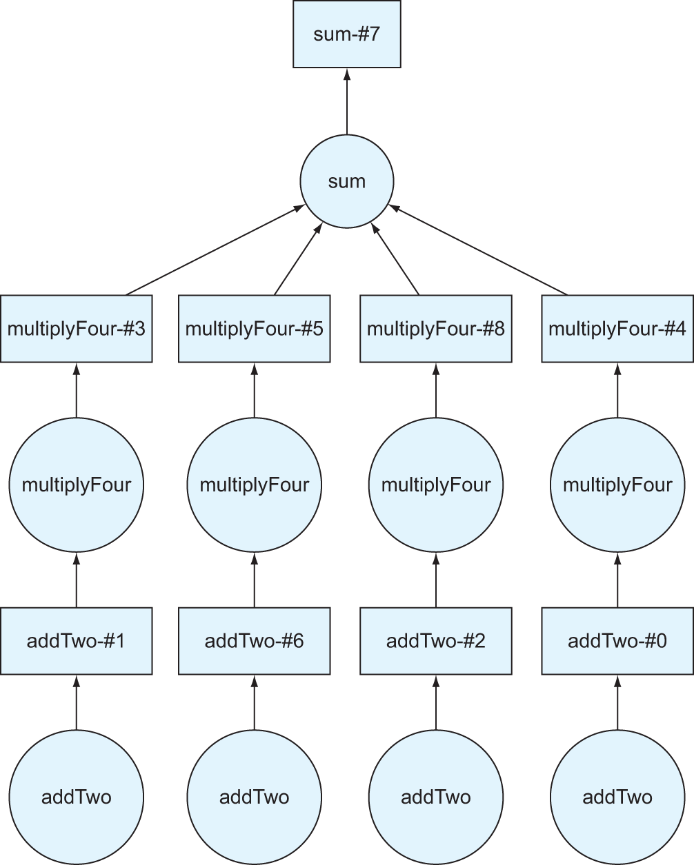
Figure 2.7 The DAG including the multiplyFour step
Figure 2.7 shows the output of the computation in listing 2.8. If you look closely at the DAG, you’ll notice another layer has been added between the addTwo nodes and the sum node. This is because we’ve now instructed Dask to take each number from the list, add two to it, then add four, and then sum the results.
2.2.3 Reducing DAG complexity with persist
Let’s now take this one step further: say we want to take this sum, add it back to each of our original numbers, then sum all that together.
Listing 2.9 Adding another layer to the DAG
data2 = [delayed(sum_two_numbers)(k, total) for k in data]
total2 = delayed(sum)(data2)
total2.visualize()
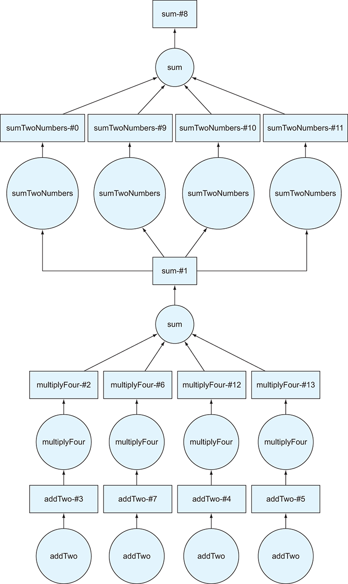
Figure 2.8 The DAG generated by listing 2.9
In this example, we’ve taken the complete DAG we created in the last example, which is stored in the total variable, and used it to create a new list of Delayed objects.
The DAG in figure 2.8 looks like the DAG from listing 2.9 was copied and another DAG was fused on top of it. That’s precisely what we want! First, Dask will calculate the sum of the first set of transformations, then add it to each of the original numbers, then finally compute the sum of that intermediate step. As you can imagine, if we repeat this cycle a few more times, the DAG will start to get too large to visualize. Similarly, if we had 100 numbers in the original list instead of 4, the DAG diagram would also be very large (try replacing the data list with a range[100] and rerun the code!) But we touched on a more important reason in the last section as to why a large DAG might become unwieldy: persistence.
As mentioned before, every time you call the compute method on a Delayed object, Dask will step through the complete DAG to generate the result. This can be okay for simple computations, but if you’re working on very large, distributed datasets, it can quickly become inefficient to repeat calculations over and over again. One way around that is to persist intermediate results that you want to reuse. But what does that do to the DAG?
Listing 2.10 Persisting calculations
total_persisted = total.persist()
total_persisted.visualize()
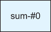
Figure 2.9 The DAG generated by listing 2.10
In this example, we took the DAG we created in listing 2.9 and persisted it. What we get instead of the full DAG is a single result, as seen in figure 2.9 (remember that a rectangle represents a result). This result represents the value that Dask would calculate when the compute method is called on the total object. But instead of re-computing it every time we need to access its value, Dask will now compute it once and save the result in memory. We can now chain another delayed calculation on top of this persisted result, and we get some interesting results.
Listing 2.11 Chaining a DAG from a persisted DAG
data2 = [delayed(sum_two_numbers)(l, total_persisted) for l in data]
total2 = delayed(sum)(data2)
total2.visualize()
The resulting DAG in figure 2.10 is much smaller. In fact, it looks like only the top half of the DAG from listing 2.9. That’s because the sum-#1 result is precomputed and persisted. So instead of calculating the whole DAG in listing 2.11, Dask can use the persisted data, thereby reducing the number of calculations needed to produce the result.
Before we move on to the next section, give listing 2.12 a try! Dask can generate very large DAGs. Although the diagram won’t fit on this page, it will hopefully give you an appreciation of the complexity that Dask can handle very elegantly.
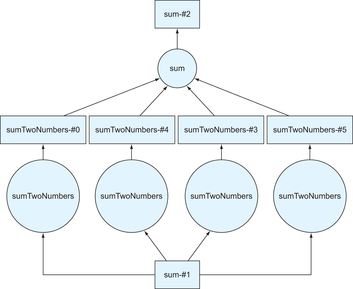
Figure 2.10 The DAG generated by listing 2.11
Listing 2.12 Visualizing the last NYC data DAG
missing_count.visualize()
2.3 Task scheduling
As I’ve mentioned a few times now, Dask uses the concept of lazy computations throughout its API. We’ve seen the effect of this in action—whenever we perform some kind of action on a Dask Delayed object, we have to call the compute method before anything actually happens. This is quite advantageous when you consider the time it might take to churn through petabytes of data. Since no computation actually happens until you request the result, you can define the complete string of transformations that Dask should perform on the data without having to wait for one computation to finish before defining the next—leaving you to do something else (like dice onions for that pot of bucatini all’Amatriciana I’ve convinced you to make) while the complete result is computing!
2.3.1 Lazy computations
Lazy computations also allow Dask to split work into smaller logical pieces, which helps avoid loading the entire data structure that it’s operating on into memory. As you saw with the DataFrame in section 2.1, Dask divided the 2 GB file into 33 64 MB chunks, and operated on 8 chunks at a time. That means the maximum memory consumption for the entire operation didn’t exceed 512 MB, yet we were still able to process the entire 2 GB file. This gets even more important as the size of the datasets you work on stretches into the terabyte and petabyte range.
But what actually happens when you request the result from Dask? The computations you defined are represented by a DAG, which is a step-by-step plan for computing the result you want. However, that step-by-step plan doesn’t define which physical resources should be used to perform the computations. Two important things still must be considered: where the computations will take place and where the results of each computation should be shipped to if necessary. Unlike relational database systems, Dask does not predetermine the precise runtime location of each task before the work begins. Instead, the task scheduler dynamically assesses what work has been completed, what work is left to do, and what resources are free to accept additional work in real time. This allows Dask to gracefully handle a host of issues that arise in distributed computing, including recovery from worker failure, network unreliability, and workers completing work at different speeds. In addition, the task scheduler can keep track of where intermediate results have been stored, allowing follow-on work to be shipped to the data instead of unnecessarily shipping the data around the network. This results in far greater efficiency when operating Dask on a cluster.
2.3.2 Data locality
Since Dask makes it easy to scale up your code from your laptop to hundreds or thousands of physical servers, the task scheduler must make intelligent decisions about which physical machine(s) will be asked to take place in a specific piece of a computation. Dask uses a centralized task scheduler to orchestrate all this work. To do this, each Dask worker node reports what data it has available and how much load it’s experiencing to the task scheduler. The task scheduler constantly evaluates the state of the cluster to come up with fair, efficient execution plans for computations submitted by users. For example, if we split the example from section 2.1 (reading the NYC parking ticket data) between two computers (server A and server B), the task scheduler may state that an operation on partition 26 should be performed by server A, and the same operation should be performed on partition 8 by server B. For the most part, if the task scheduler divides up the work as evenly as possible across machines in the cluster, the computations will complete as quickly and efficiently as possible.
But that rule of thumb does not always hold true in a number of scenarios: one server is under heavier load than the others, has less powerful hardware than the others, or does not have fast access to the data. If any of those conditions is true, the busier/weaker server will lag behind the others, and therefore should be given proportionately fewer tasks to avoid becoming a bottleneck. The dynamic nature of the task scheduler allows it to react to these situations accordingly if they cannot be avoided.
For best performance, a Dask cluster should use a distributed filesystem like S3 or HDFS to back its data storage. To illustrate why this is important, consider the following counterexample, where a file is stored on only one machine. For the sake of our example, the data is stored on server A. When server A is directed to work on partition 26, it can read the partition directly off its hard disk. However, this poses a problem for server B. Before server B can work on partition 8, server A will need to send partition 8 to server B. Any additional partitions that server B is to work on will also need to be sent over to server B before the work can begin. This will cause a considerable slowdown in the computations because operations involving networking (even 10 Gb fiber) are slower than direct reads off of locally attached disks.
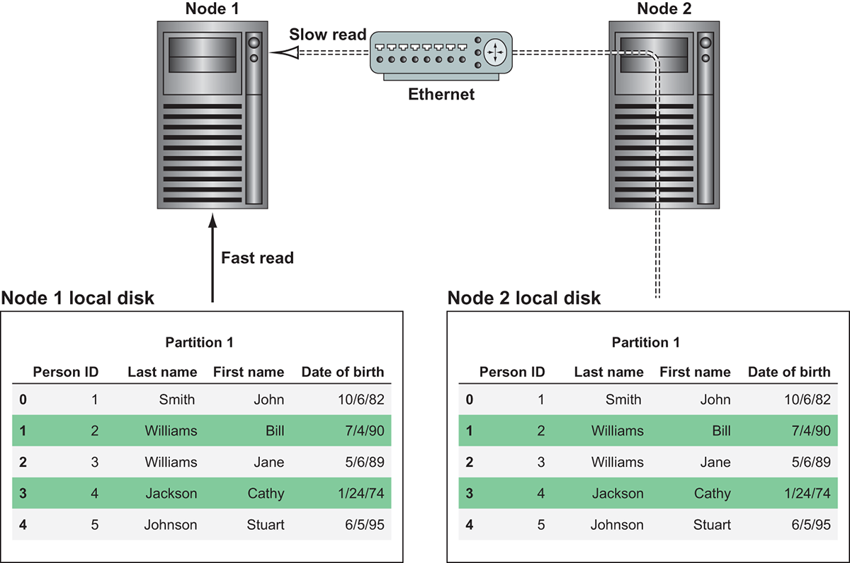
Figure 2.11 Reading data from local disk is much faster than reading data stored remotely.
Figure 2.11 demonstrates this issue. If Node 1 wants to work on Partition 1, it would be able to do so much more quickly if it had Partition 1 available on local disk. If this wasn’t an option, it could read the data over the network from Node 2, but that would be much slower.
The remedy to this problem would be to split the file up ahead of time, store some partitions on server A, and store some partitions on server B. This is precisely what a distributed file system does. Logical files are split up between physical machines. Aside from other obvious benefits, like redundancy in the event one of the servers’ hard disks fails, distributing the data across many physical machines allows the workload to be spread out more evenly. It’s far faster to bring the computations to the data than to bring the data to the computations!
Dask’s task scheduler takes data locality, or the physical location of data, into account when considering where a computation should take place. Although it’s sometimes not possible for Dask to completely avoid moving data from one worker to another, such as instances where some data must be broadcast to all machines in the cluster, the task scheduler tries its hardest to minimize the amount of data that moves between physical servers. When datasets are smaller, it might not make much difference, but when datasets are very large, the effects of moving data around the network are much more evident. Therefore, minimizing data movement generally leads to more performant computations.
Hopefully you now have a better understanding of the important role that DAGs play in enabling Dask to break up huge amounts of work into more manageable pieces. We’ll come back to the Delayed API in later chapters, but keep in mind that every piece of Dask we touch in this book is backed by Delayed objects, and you can visualize the backing DAG at any time. In practice, you likely won’t need to troubleshoot computations in such explicit detail very often, but understanding the underlying mechanics of Dask will help you better identify potential issues and bottlenecks in your workloads. In the next chapter, we’ll begin our deep dive into the DataFrame API in earnest.
Summary
- Computations on Dask DataFrames are structured by the task scheduler using DAGs.
- Computations are constructed lazily, and the
computemethod is called to execute the computation and retrieve the results. - You can call the
visualizemethod on any Dask object to see a visual representation of the underlying DAG. - Computations can be streamlined by using the
persistmethod to store and reuse intermediate results of complex computations. - Data locality brings the computation to the data in order to minimize network and IO latency.