This chapter covers

• Visualizing CNN feature maps
• Understanding the DeepDream algorithm and implementing your own dream
• Using the neural style transfer algorithm to create artistic images

In fine art, especially painting, humans have mastered the skill of creating unique visual experiences through composing a complex interplay between the content and style of an image. So far, the algorithmic basis of this process is unknown, and there exists no artificial system with similar capabilities. Nowadays, deep neural networks have demonstrated great promise in many areas of visual perception such as object classification and detection. Why not try using deep neural networks to create art? In this chapter, we introduce an artificial system based on a deep neural network that creates artistic images of high perceptual quality. The system uses neural representations to separate and recombine content and style of arbitrary images, providing a neural algorithm for the creation of artistic images.

In this chapter, we explore two new techniques to create artistic images using neural networks: DeepDream and neural style transfer. First, we examine how convolutional neural networks see the world. We’ve learned how CNNs are used to extract features in object classification and detection problems; here, we learn how to visualize the extracted feature maps. One reason is that we need this visualization technique in order to understand the DeepDream algorithm. Additionally, this will help us gain a better understanding of what our network learned during training; we can use that to improve the network’s performance when solving classification and detection problems.

Next, we discuss the DeepDream algorithm. The key idea of this technique is to print the features we visualize in a certain layer onto our input image, to create a dream-like hallucinogenic image. Finally, we explore the neural style transfer technique, which takes two images as inputs--a style image and a content image--and creates a new combined image that contains the layout from the content image and the texture, colors, and patterns from the style image.

Why is this discussion important? Because these techniques help us understand and visualize how neural networks are able to carry out difficult classification and detection tasks and check what the network has learned during training. Being able to see what the network thinks is an important feature to use when distinguishing objects will help you understand what is missing from your training set and thus improve the network’s performance.

These techniques also make us wonder whether neural networks could become tools for artists, give us a new way to combine visual concepts, or perhaps even shed a little light on the roots of the creative process in general. Moreover, these algorithms offer a path forward to an algorithmic understanding of how humans create and perceive artistic imagery.

9.1 How convolutional neural networks see the world

We have talked a lot in this book about all the amazing things deep neural networks can do. But despite all the exciting news about deep learning, the exact way neural networks see and interpret the world remains a black box. Yes, we have tried to explain how the training process works, and we explained intuitively and mathematically the backpropagation process that the network applies to update weights through many iterations to optimize the loss function. This all sounds good and makes sense on the scientific side of things. But how do CNNs see the world? How do they see the extracted features between all the layers?

A better understanding of exactly how they recognize specific patterns or objects and why they work so well might allow us to improve their performance even further. Additionally, on the business side, this would also solve the “AI explainability” problem. In many cases, business leaders feel unable to make decisions based on model predictions because nobody really understands what is happening inside the black box. This is what we do in this section: we open the black box and visualize what the network sees through its layers, to help make neural network decisions interpretable by humans.

In computer vision problems, we can visualize the feature maps inside the convolutional network to understand how they see the world and what features they think are distinctive in an object for differentiating between classes. The idea of visualizing convolutional layers was proposed by Erhan et al. in 2009.1 In this section, we will explain this concept and implement it in Keras.

9.1.1 Revisiting how neural networks work

Before we jump into the explanation of how we can visualize the activation maps (or feature maps) in a CNN, let’s revisit how neural networks work. We train a deep neural network by showing it millions of training examples. The network then gradually updates its parameters until it gives the classifications we want. The network typically consists of 10-30 stacked layers of artificial neurons. Each image is fed into the input layer, which then talks to the next layer, until eventually the “output” layer is reached. The network’s prediction is then produced by its final output layer.

One of the challenges of neural networks is understanding what exactly goes on at each layer. We know that after training, each layer progressively extracts image features at higher and higher levels, until the final layer essentially makes a decision about what the image contains. For example, the first layer may look for edges or corners, intermediate layers interpret the basic features to look for overall shapes or components, and the final few layers assemble those into complete interpretations. These neurons activate in response to very complex images such as a car or a bike.

To understand what the network has learned through its training, we want to open this black box and visualize its feature maps. One way to visualize the extracted features is to turn the network upside down and ask it to enhance an input image in such a way as to elicit a particular interpretation. Say you want to know what sort of image would result in the output “Bird.” Start with an image full of random noise, and then gradually tweak the image toward what the neural net considers an important feature of a bird (figure 9.1).

Figure 9.1 Start with an image consisting of random noise, and tweak it until we visualize what the network considers important features of a bird.

We will dive deeper into the bird example and see how to visualize the network filters. The takeaway from this introduction is that neural networks are smart enough to understand which are the important features to pass along through its layers to be classified by its fully connected layers. Non-important features are discarded along the way. To put it simply, neural networks learn the features of the objects in the training dataset. If we are able to visualize these feature maps at the deeper layers of the network, we can find out where the neural network is paying attention and see the exact features that it uses to make its predictions.

NOTE This process is described best in François Chollet’s book, Deep Learning with Python (Manning, 2017; www.manning.com/books/deep-learning-with-python): “You can think of a deep network as a multistage information-distillation operation, where information goes through successive filters and comes out increasingly purified.”

9.1.2 Visualizing CNN features

An easy way to visualize the features learned by convolutional networks is to display the visual pattern that each filter is meant to respond to. This can be done with gradient ascent in input space. By applying gradient ascent to the value of the input image of a ConvNet, we can maximize the response of a specific filter, starting from a blank input image. The resulting input image will be one that the chosen filter is maximally responsive to.

Now comes the fun part of this section. In this exercise, we will see the visualized feature maps of a few examples at the beginning, middle, and end of a VGG16 network. The implementation is straightforward, and we will get to it soon. Before we go to the code implementation, let’s take a look at what these visualized filters look like.

From the VGG16 diagram we saw in figure 9.1, let’s visualize the output feature maps of the first, middle, and deep layers as follows: block1_conv1, block3_conv2, and block5_conv3. Figures 9.2, 9.3, and 9.4 show how the features evolve throughout the network layers.

Figure 9.2 Visualizing feature maps produced by block1_conv1 filters

As you can see in figure 9.2, the early layers basically just encode low-level, generic features like direction and color. These direction and color filters then get combined into basic grid and spot textures in later layers. These textures are gradually combined into increasingly complex patterns (figure 9.3): the network starts to see some patterns that create basic shapes. These shapes are not very identifiable yet, but they are much clearer than the earlier ones.

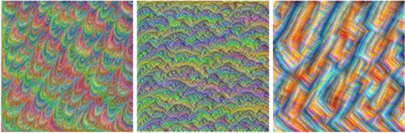
Figure 9.3 Visualizing feature maps produced by block3_conv2 filters

Now this is the most exciting part. In figure 9.4, you see that the network was able to find patterns in patterns. These features contain identifiable shapes. While the network relies on more than one feature map to make its prediction, we can look at these maps and make a close guess about the content of these images. In the left image, I can see eyes and maybe a beak, and I would guess that this is a type of bird or fish. Even if our guess is not correct, we can easily eliminate most other classes like car, boat, building, bike, and so on, because we can clearly see eyes and none of those classes have eyes. Similarly, looking at the middle image, we can guess from the patterns that this is some kind of a chain. The right image feels more like food or fruit.

Figure 9.4 Visualizing feature maps produced by block5_conv3 filters

How is this helpful in classification and detection problems? Let’s take the left feature map in figure 9.4 as an example. Looking at the visible features like eyes and beaks, I can interpret that the network relies on these two features to identify a bird. With this knowledge about what the network learned about birds, I will guess that it can detect the bird in figure 9.5, because the bird’s eye and beak are visible.

Figure 9.5 Example of a bird image with visible eye and beak features

Now, let’s consider a more adversarial case where we can see the bird’s body but the eye and beak are covered by leaves (figure 9.6). Given that the network adds high weights on the eye and beak features to recognize a bird, there is a good chance that it might miss this bird because the bird’s main features are hidden. On the other hand, an average human can easily detect the bird in the image. The solution to this problem is using one of several data-augmentation techniques and collecting more adversarial cases in your training dataset to force the network to add higher weights on other features of a bird, like shape and color.

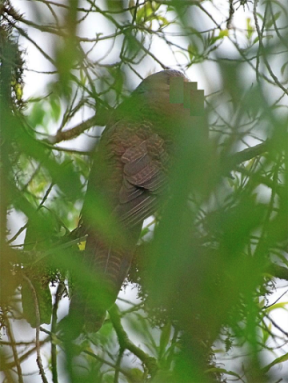
Figure 9.6 Example of an adversarial image of a bird where the eye and beak are not visible but the body is recognizable by a human

9.1.3 Implementing a feature visualizer

Now that you’ve seen the visualized examples, it is time to get your hands dirty and develop the code to visualize these activation filters yourself. This section walks through the CNN visualization code implementation from the official Keras documentation, with minor tweaking.2 You will learn how to generate patterns that maximize the mean activation of a chosen feature map. You can see the full code in Keras’s Github repository (http://mng.bz/Md8n).

NOTE You will run into errors if you try to run the code snippets in this section. These snippets are just meant to illustrate the topic. You are encouraged to check out the full executable code that is downloadable with the book.

First, we load the VGG16 model from the Keras library. To do that, we first import VGG16 from Keras and then load the model, which is pretrained on the ImageNet dataset, without including the classification fully connected layers (top part) of the network:

from keras.applications.vgg16 import VGG16                ❶
model = VGG16(weights='imagenet', include_top=False)      ❷

❶ Imports the VGG model from Keras

❷ Loads the model

Now, let’s view the names and output shape of all the VGG16 layers. We do that to pick the specific layer whose filters we want to visualize:

for layer in model.layers:                      ❶
    if 'conv' not in layer.name:                ❷
        continue
    filters, biases = layer.get_weights()       ❸
    print(layer.name, layer.output.shape)

❶ Loops through the model layers

❷ Checks for a convolutional layer

❸ Gets the filter weights

When you run this code cell, you will get the output shown in figure 9.7. These are all the convolutional layers contained in the VGG16 network. You can visualize any of their outputs simply by referring to each layer by name, as you will see in the next code snippet.

Figure 9.7 Output showing convolution layers in the downloaded VGG16 network

Let’s say we want to visualize the first conv layer: block1_conv1. Note that this layer has 64 filters, each of which has an index from 0 to 63 called filter_index. Now let’s define a loss function that seeks to maximize the activation of a specific filter (filter _index) in a specific layer (layer_name). We also want to compute the gradient using Keras’s backend function gradients and normalize the gradient to avoid very small and very large values, to ensure a smooth gradient ascent process.

In this code snippet, we set the stage for gradient ascent. We define a loss function, compute the gradients, and normalize the gradients:

from keras import backend as K
 
layer_name = 'block1_conv1'
filter_index = 0                                                          ❶
 
layer_dict = dict([(layer.name, layer) for layer in model.layers[1:]])    ❷
 
layer_output = layer_dict[layer_name].output                              ❸
loss = K.mean(layer_output[:, :, :, filter_index])                        ❸
 
grads = K.gradients(loss, input_img)[0]                                   ❹
 
grads /= (K.sqrt(K.mean(K.square(grads))) + 1e-5)                         ❺
 
iterate = K.function([input_img], [loss, grads])                          ❻

❶ Identifies the filter that we want to visualize. This can be any integer from 0 to 63, as there are 64 filters in that layer.

❷ Gets the symbolic outputs of each key layer (we gave them unique names).

❸ Builds a loss function that maximizes the activation of the nth filter of the layer considered

❹ Computes the gradient of the input picture with respect to this loss

❺ Normalizes the gradient

❻ This function returns the loss and grads given the input picture.

We can use the Keras function that we just defined to do gradient ascent to our filter activation loss:

import numpy as np
 
input_img_data = np.random.random((1, 3, img_width, img_height)) * 20 + 128  ❶
for i in range(20):                                                          ❷
    loss_value, grads_value = iterate([input_img_data])                      ❷
    input_img_data += grads_value * step                                     ❷

❶ Starts from a gray image with some noise

❷ Runs gradient ascent for 20 steps

Now that we have implemented the gradient ascent, we need to build a function that converts the tensor into a valid image. We will call it deprocess_image(x). Then we save the image on disk to view it:

from keras.preprocessing.image import save_img
 
def deprocess_image(x): 
    x -= x.mean()                              ❶
    x /= (x.std() + 1e-5)                      ❶
    x *= 0.1                                   ❶
 
    x += 0.5                                   ❷
    x = np.clip(x, 0, 1)                       ❷
 
    x *= 255                                   ❸
    x = x.transpose((1, 2, 0))                 ❸
    x = np.clip(x, 0, 255).astype('uint8')     ❸
    return x                                   ❸
 
img = input_img_data[0]
img = deprocess_image(img)
imsave('%s_filter_%d.png' % (layer_name, filter_index), img)

❶ Normalizes the tensor: centers on 0. and ensures that std is 0.1

❷ Clips to [0, 1]

❸ Converts to an RGB array

The result should be something like figure 9.8.

Figure 9.8 VGG16 layer block1_conv1 visualized

You can try to change the visualized filters to deeper layers in later blocks like block2 and block3 to see more defined features extracted as a result of the network recognizing patterns within patterns through its layers. In the highest layers (block5_conv2, block5_conv3) you will start to recognize textures similar to those found in the objects the network was trained to classify, such as feathers, eyes, and so on.

9.2 DeepDream

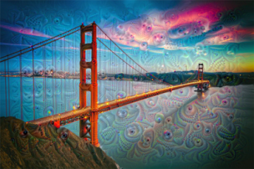
DeepDream was developed by Google researchers Alexander Mordvintsev et al. in 2015.3 It is an artistic image modification technique that creates dream-like, hallucinogenic images using CNNs, as shown in the example in figure 9.9).

Figure 9.9 DeepDream output image

For comparison, the original input image is shown in figure 9.10. The original is a scenic image from the ocean, containing two dolphins and other creatures. DeepDream merged both dolphins into one object and replaced one of the faces with what looks like a dog face. Other objects were also deformed in an artistic way, and the sea background has an edge-like texture.

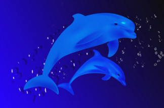
Figure 9.10 DeepDream input image

DeepDream quickly became an internet sensation, thanks to the trippy pictures it generates, full of algorithmic artifacts, bird feathers, dog faces, and eyes. These artifacts are byproducts of the fact that the DeepDream ConvNet was trained on ImageNet, where dog breeds and bird species are vastly overrepresented. If you tried another network that was pretrained on a dataset with a majority distribution of other objects, such as cars, you would see car features in your output image.

The project started as a fun experiment to run a CNN in reverse and visualize its activation maps using the same convolutional filter-visualization techniques explained in section 9.1: run a ConvNet in reverse, doing gradient ascent on the input in order to maximize the activation of a specific filter in an upper layer of the ConvNet. DeepDream uses this same idea, with a few alterations:

• Input image --In filter visualization, we don’t use an input image. We start from a blank image (or a slightly noisy one) and then maximize the filter activations of the convolutional layers to view their features. In DeepDream, we use an input image to the network because the goal is to print these visualized features on an image.

• Maximizing filters versus layers --In filter visualization, as the name implies, we only maximize activations of specific filters within the layer. But in DeepDream, we aim to maximize the activation of the entire layer to mix together a large number of features at once.

• Octaves --In DeepDream, the input images are processed at different scales called octaves to improve the quality of the visualized features. This process will be explained next.

9.2.1 How the DeepDream algorithm works

Similar to the filter-visualization technique, DeepDream uses a pretrained network on a large dataset. The Keras library has many pretrained ConvNets available to use: VGG16, VGG19, Inception, ResNet, and so on. We can use any of these networks in the DeepDream implementation; we can even train a custom network on our own dataset and use it in the DeepDream algorithm. Intuitively, the choice of network and the data it is pretrained on will affect our visualizations because different ConvNet architectures result in different learned features; and, of course, different training datasets will create different features as well.

The creators of DeepDream used an Inception model because they found that in practice, it produces nice-looking dreams. So in this chapter, we will use the Inception v3 model. You are encouraged to try different models to observe the difference.

The overall idea with DeepDream is that we pass an input image through a pretrained neural network such as the Inception v3 model. At some layer, we calculate the gradient, which tells us how we should change the input image to maximize the value at this layer. We continue doing this for 10, 20, or 40 iterations until eventually, patterns start to emerge in the input image (figure 9.11).

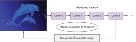
Figure 9.11 DeepDream algorithm

This works fine, except that if the pretrained network has been trained on fairly small image sizes, like ImageNet, then when our input image is large (say, 1000 × 1000), the DeepDream algorithm will print a lot of small patterns in the image that look noisy rather than artistic. This happens because all the extracted features are small in size. To solve this problem, the DeepDream algorithm processes the input image at different scales called octaves.

Octave is just a fancy word for an interval. The idea is to apply the DeepDream algorithm on the input image through intervals. We first downscale the image several times into different scales. The number of scales is configurable, as you will see soon. For each interval, we do the following:

1. Inject details: to avoid losing a lot of image details after each successive scale-up, we re-inject the lost details back into the image after each upscale process to create a blended image.

2. Apply the DeepDream algorithm: send the blended image through the DeepDream algorithm.

3. Upscale to the next interval.

As you can see in figure 9.12, we start with the large input image and then downscale two times to get a small image in octave 3. For the first interval of applying DeepDream, we don’t need to do detail injection because the input image is the source image that hasn’t been upscaled before. We pass it through the DeepDream algorithm and then upscale the output. After upscaling, details are lost, which results in an increasingly blurry or pixelated image. This is why it is valuable to re-inject the image details from the input image in octave 2 and then pass the blended image through the DeepDream algorithm. We apply the same process of upscale, detail injection, and DeepDream one more time to get the final result image. This process is run recursively for an identified number of iterations until we are satisfied with the output art.

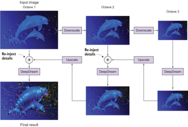
Figure 9.12 The DeepDream process: successive image downscales called octaves, detail re-injection, and then upscaling to the next octave

We set the DeepDream parameters as follows:

num_octave = 3           ❶
 
octave_scale = 1.4       ❷
 
iterations = 20          ❸

❶ Number of scales

❷ Size ratio between scales. Each successive scale is larger than the previous one by a factor of 1.4 (40% larger).

❸ Number of iterations

Now that you understand how the DeepDream algorithm works, let’s take a look at DeepDream in action using Keras.

9.2.2 DeepDream implementation in Keras

The DeepDream implementation that we are going to implement is based on François Chollet’s code from the official Keras documentation (https://keras.io/examples/ generative/deep_dream/) and his book, Deep Learning with Python. We’ll explain this code after adapting it to work on Jupyter Notebooks:

import numpy as np
from keras.applications import inception_v3
from keras import backend as K
from keras.preprocessing.image import save_img
 
K.set_learning_phase(0)                                                     ❶
 
model = inception_v3.InceptionV3(weights='imagenet', include_top=False)     ❷

❶ Disables all training operations since we won’t be doing any training with the model

❷ Downloads the pretrained Inception v3 model without its top part

Now, we need to define a dictionary that specifies which layers are used to generate the dream. To do that, let’s print out the model summary to view all the layers and select the layers names:

model.summary()

Inception v3 is very deep, and the summary printout is long. For simplicity, figure 9.13 shows a few layers of the network.

The exact layers you choose and their contribution to the final loss have an important influence on the visuals you can produce in the dream image, so you want to make these parameters easily configurable. To define the layers that we want to contribute to the dream creation, we create a dictionary with the layer names and their respective weights. The larger the weight of the layer, the higher its level of contribution to the dream:

layer_contributions = {
                        'mixed2': 0.4,
                        'mixed3': 2.,
                        'mixed4': 1.5,
                        'mixed5': 2.3,
                      }

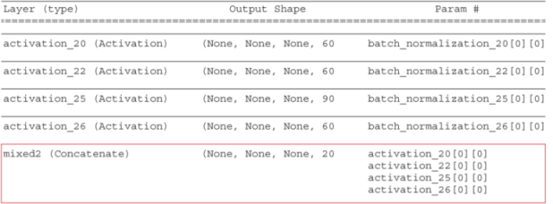
Figure 9.13 Part of the Inception v3 model summary

These are the names of the layers for which we try to maximize activations. Note that when you change the layers in this dictionary, you will produce different dreams, so you are encouraged to experiment with different layers and their corresponding weights. For this project, we will start with a somewhat arbitrary configuration by adding four layers to our dictionary and their weights: mixed2, mixed3, mixed4, and mixed5. As a guide, remember from earlier in this chapter that lower layers can be used to generate edges and geometric patterns, while high layers result in the injection of trippy visual patterns, including hallucinations of dogs, cats, and birds.

Now, let’s define a tensor that contains the loss: the weighted sum of the L2 norm of the activations of the layers:

layer_dict = dict([(layer.name, layer) for layer in model.layers])      ❶
 
loss = K.variable(0.)                                                   ❷
 
for layer_name in layer_contributions:
    coeff = layer_contributions[layer_name]
    activation = layer_dict[layer_name].output
    scaling = K.prod(K.cast(K.shape(activation), 'float32'))
    
    loss = loss + coeff * 
        K.sum(K.square(activation[:, 2: -2, 2: -2, :])) / scaling       ❸

❶ Dictionary that maps layer names to layer instances

❷ Defines the loss by adding layer contributions to this scalar variable

❸ Adds the L2 norm of the features of a layer to the loss. We avoid border artifacts by only involving non-border pixels in the loss.

Next, we compute the loss, which is the quantity we will try to maximize during the gradient ascent process. In filter visualization, we wanted to maximize the value of a specific filter in a specific layer. Here, we will simultaneously maximize the activation of all filters in a number of layers. Specifically, we will maximize a weighted sum of the L2 norm of the activations of a set of high-level layers:

dream = model.input                                           ❶
 
grads = K.gradients(loss, dream)[0]                           ❷
 
grads /= K.maximum(K.mean(K.abs(grads)), 1e-7)                ❸
 
outputs = [loss, grads]                                       ❹
fetch_loss_and_grads = K.function([dream], outputs)           ❹
 
def eval_loss_and_grads(x):
    outs = fetch_loss_and_grads([x])
    loss_value = outs[0]
    grad_values = outs[1]
    return loss_value, grad_values
def gradient_ascent(x, iterations, step, max_loss=None):      ❺
    for i in range(iterations):
        loss_value, grad_values = eval_loss_and_grads(x)
        if max_loss is not None and loss_value > max_loss:
            break
        print('...Loss value at', i, ':', loss_value)
        x += step * grad_values
    return x

❶ Tensors that holds the generated image

❷ Computes the gradients of the dream image with regard to the loss

❸ Normalizes the gradients

❹ Sets up a Keras function to retrieve the value of the loss and gradients given an input image

❺ Runs the gradient ascent process for a number of iterations

Now we are ready to develop our DeepDream algorithm. The process is as follows:

1. Load the input image.

2. Define the number of scales, from smallest to largest.

3. Resize the input image to the smallest scale.

4. For each scale, start with the smallest and apply the following:

   • Gradient ascent function
   • Upscaling to the next scale
   • Re-injecting details that were lost during the upscale process

   • Stop the process when we are back to the original size.

First, we set the algorithm parameters:

step = 0.01              ❶
num_octave = 3           ❷
octave_scale = 1.4       ❸
iterations = 20          ❹
max_loss = 10.

❶ Gradient ascent step size

❷ Number of scales at which we run gradient ascent

❸ Size ratio between scales

❹ Number of iterations

Note that playing with these hyperparameters will allow you to achieve new effects.

Let’s define the input image that we want to use to create our dream. For this example, I downloaded an image of the Golden Gate Bridge in San Francisco (see figure 9.14); feel free to use an image of your own. Figure 9.15 shows the DeepDream output image.

Figure 9.14 Example input image

Figure 9.15 DeepDream output

Here’s the Keras code:

base_image_path = 'input.jpg'                      ❶
img = preprocess_image(base_image_path)
original_shape = img.shape[1:3]
 
successive_shapes = [original_shape]
 
for i in range(1, num_octave):
    shape = tuple([int(dim / (octave_scale ** i)) for dim in original_shape])
    successive_shapes.append(shape)
successive_shapes = successive_shapes[::-1]
original_img = np.copy(img)
shrunk_original_img = resize_img(img, successive_shapes[0])
for shape in successive_shapes:
    print('Processing image shape', shape)
    
    img = resize_img(img, shape)
    img = gradient_ascent(img, iterations=iterations, step=step, 
                          max_loss=max_loss)
    upscaled_shrunk_original_img = resize_img(shrunk_original_img, shape)
    same_size_original = resize_img(original_img, shape)
    lost_detail = same_size_original - upscaled_shrunk_original_img
    img += lost_detail
    shrunk_original_img = resize_img(original_img, shape)
    
    phil_img = deprocess_image(np.copy(img))
    save_img('deepdream_output/dream_at_scale_' + str(shape) + '.png', phil_img)
 
final_img = deprocess_image(np.copy(img))
save_img('final_dream.png', final_img)              ❷

❶ Defines the path to the input image

❷ Saves the result to disk

9.3 Neural style transfer

So far, we have learned how to visualize specific filters in a network. We also learned how to manipulate features of an input image to create dream-like hallucinogenic images using the DeepDream algorithm. In this section, we explore a new type of artistic image that ConvNets can create using neural style transfer : the technique of transferring the style from one image to another.

The goal of the neural style transfer algorithm is to take the style of an image (style image) and apply it to the content of another image (content image). Style in this context means texture, colors, and other visual patterns in the image. And content is the higher-level macrostructure of the image. The result is a combined image that contains both the content of the content image and the style of the style image.

For example, let’s look at figure 9.16. The objects in the content image (like dolphins, fish, and plants) are kept in the combined image but with the specific texture of the style image (blue and yellow brushstrokes).

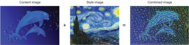
Figure 9.16 Example of neural style transfer

The idea of neural style transfer was introduced by Leon A. Gatys et al. in 2015.4 The concept of style transfer, which is tightly related to texture generation, had a long history in the image-processing community prior to that; but as it turns out, the DL-based implementations of style transfer offer results unparalleled by what had been previously achieved with traditional CV techniques, and they triggered an amazing renaissance in creative CV applications.

Among the different neural network techniques that create art (like DeepDream), style transfer is the closest to my heart. DeepDream can create cool hallucination-like images, but it can be disturbing sometimes. Plus, as a DL engineer, it is not easy to intentionally create a specific piece of art that you have in your mind. Style transfer, on the other hand, can use an artistic engineer to mix the content that you want from an image with your favorite painting to create something that you have imagined. It is a really cool technique that, if used by an artist engineer, can be used to create beautiful art on par with that produced by professional painters.

The main idea behind implementing style transfer is the same as the one central to all DL algorithms, as explained in chapter 2: we first define a loss function to define what we aim to achieve, and then we work on optimizing this function. In style-transfer problems, we know what we want to achieve: conserving the content of the original image while adopting the style of the reference image. Now all we need to do is to define both content and style in a mathematical representation, and then define an appropriate loss function to minimize.

The key notion in defining the loss function is to remember that we want to preserve content from one image and style from another:

• Content loss --Calculate the loss between the content image and the combined image. Minimizing this loss means the combined image will have more content from the original image.

• Style loss --Calculate the loss in style between the style image and the combined image. Minimizing this loss means the combined image will have style similar to the style image.

• Noise loss --This is called the total variation loss. It measures the noise in the combined image. Minimizing this loss creates an image with a higher spatial smoothness.

Here is the equation of the total loss:

total_loss = [style(style_image) - style(combined_image)] + 
    [content(original_image) - content(combined_image)] + total_variation_loss

NOTE Gatys et al. (2015) on transfer learning does not include the total variation loss. After experimentation, the researchers found that the network generated better, more aesthetically-pleasing style transfers when they encouraged spatial smoothness across the output image.

Now that we have a big-picture idea of how the neural style transfer algorithm works, we are going to dive deeper into each type of loss to see how it is derived and coded in Keras. We will then understand how to train a neural style transfer network to minimize the total_loss function that we just defined.

9.3.1 Content loss

The content loss measures how different two images are in terms of subject matter and the overall placement of content. In other words, two images that contain similar scenes should have a smaller loss value than two images that contain completely different scenes. Image subject matter and content placement are measured by scoring images based on higher-level feature representations in the ConvNet, such as dolphins, plants, and water. Identifying these features is the whole premise behind deep neural networks: these networks are trained to extract the content of an image and learn the higher-level features at the deeper layers by recognizing patterns in simpler features from the previous layers. With that said, we need a deep neural network that has been trained to extract the features of the content image so that we can tap into a deep layer of the network to extract high-level features.

To calculate the content loss, we measure the mean squared error between the output for the content image and the combined image. By trying to minimize this error, the network tries to add more content to the combined image to make it more and more similar to the original content image:

Content loss = 1/2 Σ[content(original_image) - content(combined_image)]²

Minimizing the content loss function ensures that we preserve the content of the original image and create it in the combined image.

To calculate the content loss, we feed both the content and style images into a pretrained network and select a deep layer from which to extract high-level features. We then calculate the mean squared error between both images. Let’s see how we calculate the content loss between two images in Keras.

NOTE The code snippets in this section are adapted from the neural style transfer example in the official Keras documentation (https://keras.io/examples/ generative/neural_style_transfer/). If you want to re-create this project and experiment with different parameters, I suggest that you work from Keras’ Github repository as a starting point (http://mng.bz/GVzv) or run the adapted code available for download with this book.

First, we define two Keras variables to hold the content image and style image. And we create a placeholder tensor that will contain the generated combined image:

content_image_path = '/path_to_images/content_image.jpg'              ❶
style_image_path = '/path_to_images/style_image.jpg'                  ❶
 
content_image = K.variable(preprocess_image(content_image_path))      ❷
style_image = K.variable(preprocess_image(style_image_path))          ❷
combined_image = K.placeholder((1, img_nrows, img_ncols, 3))          ❷

❶ Paths to the content and style images

❷ Gets tensor representations of our images

Now, we concatenate the three images into one input tensor and feed it to the VGG19 neural network. Note that when we load the VGG19 model, we set the include_top parameter to False because we don’t need to include the classification fully connected layers for this task. This is because we are only interested in the feature-extraction part of the network:

input_tensor = K.concatenate([content_image, style_image, 
                             combined_image], axis=0)           ❶
 
model = vgg19.VGG19(input_tensor=input_tensor, 
                    weights='imagenet', include_top=False)      ❷

❶ Combines the three images into a single Keras tensor

❷ Builds the VGG19 network with our three images as input. The model will be loaded with pretrained ImageNet weights.

Similar to what we did in section 9.1, we now select the network layer we want to use to calculate the content loss. We wanted to choose a deep layer to make sure it contains higher-level features of the content image. If you choose an earlier layer of the network (like block 1 or block 2), the network won’t be able to transfer the full content from the original image because the earlier layers extract low-level features like lines, edges, and blobs. In this example, we choose the second convolutional layer in block 5 (block5_conv2):

outputs_dict = dict([(layer.name, layer.output) for layer in model.layers])  ❶
layer_features = outputs_dict['block5_conv2']                                ❶

❶ Gets the symbolic outputs of each key layer (we gave them unique names)

Now we can extract the features from the layer that we chose from the input tensor:

content_image_features = layer_features[0, :, :, :]
combined_features = layer_features[2, :, :, :]

Finally, we create the content_loss function that calculates the mean squared error between the content image and the combined image. We create an auxiliary loss function designed to preserve the features of the content_image and transfer it to the combined-image:

def content_loss(content_image, combined_image):                        ❶
    return K.sum(K.square(combined - base))
 
content_loss = content_weight * content_loss(content_image_features,
                                             combined_features)         ❷

❶ Mean square error function between the content image output and the combined image

❷ content_loss is scaled by a weighting parameter.

content_weight = content_weight
style_weight = style_weight

9.3.2 Style loss

As we mentioned before, style in this context means texture, colors, and other visual patterns in the image.

Multiple layers to represent style features

Defining the style loss is a little more challenging than what we did with the content loss. In the content loss, we cared only about the higher-level features that are extracted at the deeper levels, so we only needed to choose one layer from the VGG19 network to preserve its features. In style loss, on the other hand, we want to choose multiple layers because we want to obtain a multi-scale representation of the image style. We want to capture the image style at lower-level layers, mid-level layers, and higher-level layers. This allows us to capture the texture and style of our style image and exclude the global arrangement of objects in the content image.

Gram matrix to measure jointly activated feature maps

The gram matrix is a method that is used to numerically measure how much two feature maps are jointly activated. Our goal is to build a loss function that captures the style and texture of multiple layers in a CNN. To do that, we need to compute the correlations between the activation layers in our CNN. This correlation can be captured by computing the gram matrix--the feature-wise outer product--between the activations.

To calculate the gram matrix of the feature map, we flatten the feature map and calculate the dot product:

def gram_matrix(x):
    features = K.batch_flatten(K.permute_dimensions(x, (2, 0, 1)))
    gram = K.dot(features, K.transpose(features))
    return gram

Let’s build the style_loss function. It calculates the gram matrix for a set of layers throughout the network for both the style and combined images. It then compares the similarities of style and texture between them by calculating the sum of squared errors:

def style_loss(style, combined):
    S = gram_matrix(style)
    C = gram_matrix(combined)
    channels = 3 
    size = img_nrows * img_ncols
    return K.sum(K.square(S - C)) / (4.0 * (channels ** 2) * (size ** 2))

In this example, we are going to calculate the style loss over five layers: the first convolutional layer in each of the five blocks of the VGG19 network (note that if you change the feature layers, the network will preserve different styles):

feature_layers = ['block1_conv1', 'block2_conv1',
                  'block3_conv1', 'block4_conv1',
                  'Block5_conv1']

Finally, we loop through these feature_layers to calculate the style loss:

for layer_name in feature_layers:
    layer_features = outputs_dict[layer_name]
    style_reference_features = layer_features[1, :, :, :]
    combination_features = layer_features[2, :, :, :]
    sl = style_loss(style_reference_features, combination_features)
    style_loss += (style_weight / len(feature_layers)) * sl              ❶

❶ Scales the style loss by a weighting parameter and the number of layers over which the style loss is calculated

During training, the network works on minimizing the loss between the style of the output image (combined image) and the style of the input style image. This forces the style of the combined image to correlate with the style image.

9.3.3 Total variance loss

The total variance loss is the measure of noise in the combined image. The network’s goal is to minimize this loss function in order to minimize the noise in the output image.

Let’s create the total_variation_loss function that calculates how noisy an image is. This is what we are going to do:

1. Shift the image one pixel to the right, and calculate the sum of the squared error between the transferred image and the original.

2. Repeat step 1, this time shifting the image one pixel down.

The sum of these two terms (a and b) is the total variance loss:

def total_variation_loss(x):
    a = K.square(
        x[:, :img_nrows - 1, :img_ncols - 1, :] - x[:, 1:, :img_ncols - 1, :])
    b = K.square(
        x[:, :img_nrows - 1, :img_ncols - 1, :] - x[:, :img_nrows - 1, 1:, :])
 
    return K.sum(K.pow(a + b, 1.25))
 
tv_loss = total_variation_weight * total_variation_loss(combined_image)       ❶

❶ Scales the total variance loss by the weighting parameter

Finally, we calculate the overall loss of our problem, which is the sum of the content, style, and total variance losses:

total_loss = content_loss + style_loss + tv_loss

9.3.4 Network training

Now that we have defined the total loss function for our problem, we can run the GD optimizer to minimize this loss function. First we create an object class Evaluator that contains methods that calculate the overall loss, as described previously, and gradients of the loss with respect to the input image:

class Evaluator(object):
    def __init__(self):
        self.loss_value = None
        self.grads_values = None
 
    def loss(self, x):
        assert self.loss_value is None
        loss_value, grad_values = eval_loss_and_grads(x)
        self.loss_value = loss_value
        self.grad_values = grad_values
        return self.loss_value
 
    def grads(self, x):
        assert self.loss_value is not None
        grad_values = np.copy(self.grad_values)
        self.loss_value = None
        self.grad_values = None
        return grad_values
 
evaluator = Evaluator()

Next, we use the methods in our evaluator class in the training process. To minimize the total loss function, we use the SciPy (https://scipy.org/scipylib) based optimization method scipy.optimize.fmin_l_bfgs_b:

from scipy.optimize import fmin_l_bfgs_b
 
Iterations = 1000                                                         ❶
 
x = preprocess_image(content_image_path)                                  ❷
 
for i in range(iterations):                                               ❸
    x, min_val, info = fmin_l_bfgs_b(evaluator.loss, x.flatten(),
                                     fprime=evaluator.grads, maxfun=20)
    img = deprocess_image(x.copy())                                       ❹
    fname = result_prefix + '_at_iteration_%d.png' % i                    ❹
    save_img(fname, img)                                                  ❹

❶ Trains for 1,000 iterations

❷ The training process is initialized with content_image as the first iteration of the combined image.

❸ Runs scipy-based optimization (L-BFGS) over the pixels of the generated image to minimize total_loss.

❹ Saves the current generated image

TIP When training your own neural style transfer network, keep in mind that content images that do not require high levels of detail work better and are known to create visually appealing or recognizable artistic images. In addition, style images that contain a lot of textures are better than flat style images: flat images (like a white background) will not produce aesthetically appealing results because there is not much texture to transfer.

Summary

• CNNs learn the information in the training set through successive filters. Each layer of the network deals with features at a different level of abstraction, so the complexity of the features generated depends on the layer’s location in the network. Earlier layers learn low-level features; the deeper the layer is in the network, the more identifiable the extracted features are.

• Once a network is trained, we can run it in reverse to adjust the original image slightly so that a given output neuron (such as the one for faces or certain animals) yields a higher confidence score. This technique can be used for visualizations to better understand the emergent structure of the neural network and is the basis for the DeepDream concept.

• DeepDream processes the input image at different scales called octaves. We pass each scale, re-inject image details, pass it through the DeepDream algorithm, and then upscale the image for the next octave.

• The DeepDream algorithm is similar to the filter-visualization algorithm. It runs the ConvNet in reverse to generate output based on the representations extracted by the network.

• DeepDream differs from filter-visualization in that it needs an input image and maximizes the entire layer, not specific filters within the layer. This allows DeepDream to mix together a large number of features at once.

• DeepDream is not specific to images--it can be used for speech, music, and more.

• Neural style transfer is a technique that trains the network to preserve the style (texture, color, patterns) of the style image and preserve the content of the content image. The network then creates a new combined image that combines the style of the style image and the content from the content image.

• Intuitively, if we minimize the content, style, and variation losses, we get a new image that contains low variance in content and style from the content and style images, respectively, and low noise.

• Different values for content weight, style weight, and total variation weight will give you different results.

1.Dumitru Erhan, Yoshua Bengio, Aaron Courville, and Pascal Vincent. “Visualizing Higher-Layer Features of a Deep Network.” University of Montreal 1341 (3): 1. 2009. http://mng.bz/yyMq.

2.François Chollet, “How convolutional neural networks see the world,” The Keras Blog, 2016, https://blog .keras.io/category/demo.html.

3.Alexander Mordvintsev, Christopher Olah, and Mike Tyka, “Deepdream--A Code Example for Visualizing Neural Networks,” Google AI Blog, 2015, http://mng.bz/aROB.

4.Leon A. Gatys, Alexander S. Ecker, and Matthias Bethge, “A Neural Algorithm of Artistic Style,” 2015, http:// arxiv.org/abs/1508.06576.