
- Expressing similarity between images via loss functions
- Training CNNs to achieve a desired embedding function with high accuracy
- Using visual embeddings in real-world applications
Obtaining meaningful relationships between images is a vital building block for many applications that touch our lives every day, such as face recognition and image search algorithms. To tackle such problems, we need to build an algorithm that can extract relevant features from images and subsequently compare them using their corresponding features.
Ratnesh Kumar obtained his PhD from the STARS team at Inria, France, in 2014. While working on his PhD, he focused on problems in video understanding: video segmentation and multiple object tracking. He also has a Bachelor of Engineering from Manipal University, India, and a Master of Science from the University of Florida at Gainesville. He has co-authored several scientific publications on learning visual embedding for re-identifying objects in camera networks.
In the previous chapters, we learned that we can use convolutional neural networks (CNNs) to extract meaningful features for an image. This chapter will use our understanding of CNNs to train (jointly) a visual embedding layer. In this chapter’s context, visual embedding refers to the last fully connected layer (prior to a loss layer) appended to a CNN. Joint training refers to training both the embedding layer and the CNN parameters jointly.
This chapter explores the nuts and bolts of training and using visual embeddings for large-scale, image-based query-retrieval systems such as applications of visual embeddings (see figure 10.1). To perform this task, we first need to project (embed) our database of images onto a vector space (embedding). This way, comparisons between images can be performed by measuring their pairwise distances in this embedding space. This is the high-level idea of visual embedding systems.

Figure 10.1 Example applications we encounter in everyday life when working with images: a machine comparing two images (left); querying the database to find images similar to the input image (right). Comparing two images is a non-trivial task and is key to many applications relating to meaningful image search.
DEFINITION An embedding is a vector space, typically of lower dimension than the input space, which preserves relative dissimilarity (in the input space). We use the terms vector space and embedding space interchangeably. In the context of this chapter, the last fully connected layer of a trained CNN is this vector (embedding) space. As an example, a fully connected layer of 128 neurons corresponds to a vector space of 128 dimensions.
For a reliable comparison among images, the embedding function needs to capture a desired input similarity measure. This embedding function can be learned using various approaches; one of the popular ways is to use a deep CNN. Figure 10.2 illustrates a high-level process of using CNNs to create an embedding.
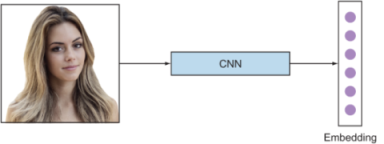
Figure 10.2 Using CNNs to obtain an embedding from an input image
In the following section, we explore some example applications of using visual embeddings for large-scale query-retrieval systems. Then we will dive deeper into the different components of the visual embedding systems: loss functions, mining informative data, and training and testing the embedding network. Subsequently, we will use these concepts to solve our chapter project on building visual embedding-based query-retrieval systems. Thereafter, we will explore approaches to push the boundaries of the project’s network accuracy. By the end of this chapter, you will be able to train a CNN to obtain a reliable and meaningful embedding and use it in real-world applications.
10.1 Applications of visual embeddings
Let’s look at some practical day-to-day information-retrieval algorithms that use the concept of visual embeddings. Some of the prominent applications for retrieving similar images given an input query include face recognition (FR), image recommendation, and object re-identification systems.
10.1.1 Face recognition
FR is about automatically identifying or tagging an image with the exact identities of persons in the image. Day-to-day applications include searching for celebrities on the web, auto-tagging friends and family in images, and many more. Recognition is a form of fine-grained classification. The Handbook of Face Recognition [1] categorizes two modes of a FR system (figure 10.3 compares them):
-
Face identification --One-to-many matches that compare a query face image against all the template images in the database to determine the identity of the query face. For example, city authorities can check a watch list to match a query to a list of suspects (one-to-few matches). Another fun example is automatically tagging users to photos they appear in, a feature implemented by major social network platforms.
-
Face verification --One-to-one match that compares a query face image against a template face image whose identity is being claimed.

Figure 10.3 Face-verification and face-recognition systems: an example of a face-verification system comparing one-on-one matches to identify whether or not the image is Sundar (left); an example of a face-identification system comparing one-to-many matches to identify all images (right). Despite the objective-level difference between recognition and identification, they both rely on a good embedding function that captures meaningful differences between faces. (The figure was inspired by [2].)
10.1.2 Image recommendation systems
In this task, the user seeks to find similar images with respect to a given query image. Shopping websites provide product suggestions (via images) based on the selection of a particular product, such as showing all kinds of shoes that are similar to the ones a user selected. Figure 10.4 shows an example in the context of apparel search.

Figure 10.4 Apparel search. The leftmost image in each row is the query image, and the subsequent columns show various apparel that look similar to it. (Images in this figure are taken from [3].)
Note that the similarity between two images varies depending on the context of choosing the similarity measure. The embedding of an image differs based on the type of similarity measure chosen. Some examples of similarity measures are color similarity and semantic similarity:
-
Color similarity --The retrieved images have similar colors, as shown in figure 10.5. This measure is used in applications like retrieving similarly colored paintings, similarly colored shoes (not necessarily determining style), and many more.
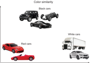
Figure 10.5 Similarity example where cars are differentiated by their color. Notice that the similarly colored cars are closer in this illustrative two-dimensional embedding space.
-
Semantic similarity --The retrieved image has the same semantic properties, as shown in figure 10.6. In our earlier example of shoe retrieval, the user expects to see suggestions of shoes having the same semantics as high-heeled shoes. You can be creative and decide to incorporate color similarity with semantics for more meaningful suggestions.

Figure 10.6 Example of identity embeddings. Cars with similar features are projected closer to each other in the embedding space.
10.1.3 Object re-identification
An example of object re-identification is security camera networks (CCTV monitoring), as depicted in figure 10.7. The security operator may be interested in querying a particular person and finding out their location in all the cameras. The system is required to identify a moving object in one camera and then re-identify the object across cameras to establish consistent identity.

Figure 10.7 Multi-camera dataset showing the presence of a person (queried) across cameras. (Source: [4].)
This problem is commonly known as person re-identification. Notice that it is similar to a face-verification system where we are interested in capturing whether any two people in separate cameras are the same, without needing to know exactly who a person is.
One of the central aspects in all these applications is the reliance on an embedding function that captures and preserves the input’s similarity (and dissimilarity) to the output embedding space. In the following sections, we will delve into designing appropriate loss functions and sampling (mining) informative data points to guide the training of a CNN for a high-quality embedding function.
But before we jump into the details of creating an embedding, let’s answer this question: why do we need to embed--can’t we just use the images directly? Let’s review the bottlenecks with this naive approach of directly using image pixel values as an embedding. Embedding dimensionality in this approach (assuming all images are high definition) would be 1920 × 1080, represented in a computer’s memory in double precision, which is computationally prohibitive for both storage and retrieval given any meaningful time requirements. Moreover, most embeddings need to be learned in a supervised setting, as a priori semantics for comparison are not known (that is when we unleash the power of CNNs to extract meaningful and relevant semantics). Any learning algorithm on such a high-dimensional embedding space will suffer from the curse of dimensionality: as the dimensionality increases, the volume of the space increases so fast that the available data becomes sparse.
The geometry and data distribution of natural data are non-uniform and concatenate around low-dimensional structures. Hence, using an image size as data dimensions is overkill (let alone the exorbitant computational complexity and redundancy). Therefore, our goal in learning embedding is twofold: learning the required semantics for comparison, and achieving a low(er) dimensionality of the embedding space.
10.2 Learning embedding
Learning an embedding function involves defining a desired criterion to measure a similarity; it can be based on color, semantics of the objects present in an image, or purely data-driven in a supervised form. Since a priori knowing the right semantics (for comparing images) is difficult, supervised learning is more popular. Instead of hand-crafting similarity criteria features, in this chapter we will focus on the supervised data-driven learning of embeddings wherein we assume we are given a training set. Figure 10.8 depicts a high-level architecture to learn an embedding using a deep CNN.

Figure 10.8 An illustration of learning machinery (top); the (test) process outline (bottom).
The process to learn an embedding is straightforward:
-
Choose a CNN architecture. Any suitable CNN architecture can be used. In practice, the last fully connected layer is used to determine the embedding. Hence the size of this fully connected layer determines the dimension of the embedding vector space. Depending on the size of the training dataset, it may be prudent to use pretraining with, for example, the ImageNet dataset.
-
Choose a loss function. Popular loss functions are contrastive and triplet loss. (These are explained in section 10.3.)
-
Choose a dataset sampling (mining) method. Naively feeding all possible samples from the dataset is wasteful and prohibitive. Hence we need to resort to sampling (mining) informative data points to train our CNN. We will learn various sampling techniques in section 10.4.
-
During test time, the last fully connected layer acts as the embedding of the corresponding image.
Now that we have reviewed the big picture of the training and inference process for learning embedding, we will delve into defining useful loss functions to express our desired embedding objectives.
10.3 Loss functions
We learned in chapter 2 that optimization problems require the definition of a loss function to minimize. Learning embedding is not different from any other DL problem: we first define a loss function that we need to minimize, and then we train a neural network to choose the parameter (weights) values that yield the minimum error value. In this section, we will look more deeply at key embedding loss functions: cross-entropy, contrastive, and triplet.
First we will formalize the problem setup. Then we will explore the different loss functions and their mathematical formulas.
10.3.1 Problem setup and formalization
To understand loss functions for learning embedding and eventually train a CNN (for this loss), let’s first formalize the input ingredients and desired output characteristics. This formalization will be used in later sections to understand and categorize various loss functions in a succinct manner. For the purposes of this conversation, our dataset can be represented as follows:
N is the number of training images, xi is the input image, and yi is its corresponding label. Our objective is to create an embedding
to map images in ℝD onto a feature (embedding) space in ℝD such that images of similar identity are metrically close in this feature space (and vice versa for images of dissimilar identities)
where θ is the parameter set of the learning function.
be the metric measuring distance of images xi, xj in the embedding space. For simplicity, we drop the input labels and denote D(xi, xj) as Dij · yij = 1. Both samples ( i ) and ( j ) belong to the same class, and the value yij = 0 indicates samples of different classes.
Once we train an embedding network for its optimal parameters, we desire the learned function to have the following characteristics:
-
An embedding should be invariant to viewpoints, illumination, and shape changes in the object.
-
From a practical application deployment, computation of embedding and ranking should be efficient. This calls for a low-dimension vector space (embedding). The bigger this space is, the more computation is required to compare any two images, which in turn affects the time complexity.
Popular choices for learning an embedding are cross-entropy loss, contrastive loss, and triplet loss. The subsequent sections will introduce and formalize these losses.
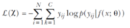
10.3.2 Cross-entropy loss
Learning an embedding can also be formulated as a fine-grained classification problem, and the corresponding CNN can be trained using the popular cross-entropy loss (explained in detail in chapter 2). The following equation expresses cross-entropy loss, where p(yij | f (x; θ )) represents the posterior class probability. In CNN literature, softmax loss implies a softmax layer trained in a discriminative regime using cross-entropy loss:
During training, a fully connected (embedding) layer is added prior to the loss layer. Each identity is considered a separate category, and the number of categories is equal to the number of identities in the training set. Once the network is trained using classification loss, the final classification layer is stripped off and an embedding is obtained from the new final layer of the network (figure 10.9).

Figure 10.9 An illustration of how cross-entropy loss is used to train an embedding layer (fully connected). The right side demonstrates the inference process and outlines the disconnect in training and inference in straightforward usage of cross-entropy loss for learning an embedding. (This figure is adapted from [5].)
By minimizing the cross-entropy loss, the parameters (θ) of the CNN are chosen such that the estimated probability is close to 1 for the correct class and close to 0 for all other classes. Since the target of the cross-entropy loss is to categorize features into predefined classes, usually the performance of such a network is poor when compared to losses incorporating similarity (and dissimilarity) constraints directly in the embedding space during training. Furthermore, learning becomes computationally prohibitive when considering datasets of, for example, 1 million identities. (Imagine a loss layer with 1 million neurons!) Nevertheless, pretraining a network with cross-entropy loss (on a viable subset of the dataset, such as a subset of 1,000 identities) is a popular strategy used to pretrain the CNN, which in turn makes embedding losses converge faster. We will explore this further while mining informative samples during training in section 10.4.
NOTE One of the disadvantages of the cross-entropy loss is the disconnect between training and inference. Hence, it generally performs poorly when compared with embedding learning losses (contrastive and triplet). These losses explicitly try to incorporate the relative distance preservation from the input image space to the embedding space.
10.3.3 Contrastive loss
Contrastive loss optimizes the training objective by encouraging all similar class instances to come infinitesimally closer to each other, while forcing instances from other classes to move far apart in the output embedding space (we say infinitesimally here because a CNN can’t be trained with exactly zero loss). Using our problem formalization, this loss is defined as
be the metric measuring distance of images xi, xj in the embedding space. For simplicity, we drop the input labels and denote D(xi, xj) as Dij · yij = 1. Both samples ( i ) and ( j ) belong to the same class, and the value yij = 0 indicates samples of different classes.
lcontrastive (i, j) = yij D2ij + (1 - yij)[α - D2ij]+
Note that [.]+ = max(0,.) in the loss function indicates hinge loss, and α is a predetermined threshold (margin) determining the max loss for when the two samples i and j are in different classes. Geometrically, this implies that two samples of different classes contribute to the loss only if the distance between them in the embedding space is less than this magin. Dij, as noted in the formulation, refers to the distance between two samples i and j in the embedding space.
This loss is also known as Siamese loss, because we can visualize this as a twin network with shared parameters; each of the two CNNs is fed an image. Contrastive loss was employed in the seminal work by Chopra et al. [6] for the face-verification problem, where the objective is to verify whether two presented faces belong to the same identity. An illustration of this loss is provided in the context of face recognition in figure 10.10.

Figure 10.10 Computing contrastive loss requires two images. When the two images are of the same class, the optimization tries to put them closer in the embedding space, and vice versa when the images belong to different classes.
Notice that the choice of the margin α is the same for all dissimilar classes. Manmatha et al. [7] analyze the impact: this choice of α implies that for dissimilar identities, visually diverse classes are embedded in the same feature space as the visually similar ones. This assumption is stricter when compared to triplet loss (explained next) and restricts the structure of the embedding manifold, which subsequently makes learning tougher. The training complexity per epoch is O(N 2) for a dataset of N samples, as this loss requires traversing a pair of samples to compute the contrastive loss.
10.3.4 Triplet loss
Inspired by the seminal work on metric learning for nearest neighbor classification by Weinberger et al. [8], FaceNet (Schroff et al. [9]) proposed a modification suited for query-retrieval tasks called triplet loss. Triplet loss forces data points from the same class to be closer to each other than they are to a data point from another class. Unlike contrastive loss, triplet loss adds context to the loss function by considering both positive and negative pair distances from the same point. Mathematically, with respect to our problem formalization from earlier, triplet loss can be formulated as follows:
ltriplet (a, p, n) = [Dap − Dan + α]+
Note that Dap represents the distance between the anchor and a positive sample, while Dan is the distance between the anchor and a negative sample. Figure 10.11 illustrates the computation of the loss term using an anchor, a positive sample, and a negative sample. Upon successful training, the hope is that we will get all the same class pairs closer than pairs from different classes.
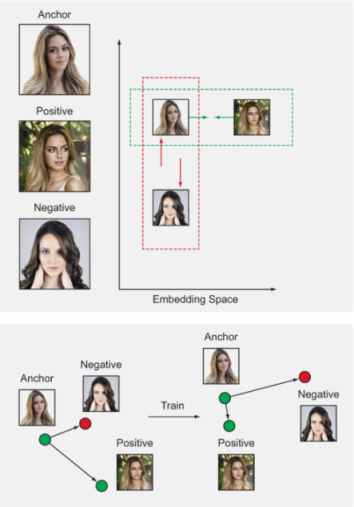
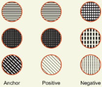
Figure 10.11 Computing triplet loss requires three samples. The goal of learning is to embed the samples of the same class closer than samples belonging to different classes.
Because computing triplet loss requires three terms, the training complexity per epoch is O(N3), which is computationally prohibitive on practical datasets. High computational complexity in triplet and contrastive losses have motivated a host of sampling approaches for efficient optimization and convergence. Let’s review the complexity of implementing these losses in a naive and straightforward manner.
10.3.5 Naive implementation and runtime analysis of losses
Consider a toy example with the following specifications:
If we implement the losses in a naive manner (see figure 10.12), it leads to per-epoch (inner for loop,1 in figure 10.12) training complexity:
-
Cross-entropy loss --This is a relatively straightforward loss. In an epoch, it just needs to traverse all samples. Hence our complexity here is O(N × S) = O(103).
-
Contrastive loss --This loss visits all pairwise distances, so complexity is quadratic in terms of number of samples (N × S): that is, O(100 × 10 × 100 × 10) = O(106).
-
Triplet loss --For every loss computation, we need to visit three samples, so the worst-case complexity is cubic. In terms of total number of samples, that is O(109).

Figure 10.12 Algorithm 1, for a naive implementation
Despite the ease of computing cross-entropy loss, its performance is relatively low when compared to other embedding losses. Some intuitive explanations are pointed out in section 10.3.2. In recent academic works (such as [10, 11, 13]), triplet loss has generally given better results than contrastive loss when provided with appropriate hard data mining, which we will explain in the next section.
NOTE In the following sections, we refer to triplet loss, owing to its high performance over contrastive loss in several academic works.
One important point to notice is that not many of the triplets of the O(109) contribute to the loss in a strong manner. In practice, during a training epoch, most of the triplets are trivial: that is, the current network is already at a low loss on these, and hence anchor-positive pairs of these trivial triplets are much closer (in the embedding space) than anchor-negative pairs. These trivial triplets do not add meaningful information to update the network parameters, thereby stagnating convergence. Furthermore, there are far fewer informative triplets than trivial triplets, which in turn leads to washing out the contribution of informative triplets.
To improve the computational complexity of triplet enumeration and convergence, we need to come up with an efficient strategy for enumerating triplets and feed the CNN (during training) informative triplet samples (without trivial triplets). This process of selecting informative triplets is called mining. Informative data points is the essence of this chapter and is discussed in the following sections.
A popular strategy to tackle this cubic complexity is to enumerate triplets in the following manner:
The next section looks at this strategy in detail.
10.4 Mining informative data
So far, we have looked at how triplet and contrastive losses are computationally prohibitive for practical dataset sizes. In this section, we take a deep dive into understanding the key steps during training a CNN for triplet loss and learn how to improve the training convergence and computational complexity.
The straightforward implementation in figure 10.12 is classified under offline training, as the selection of a triplet must consider the full dataset and therefore cannot be done on the fly while training a CNN. As we noted earlier, this approach of computing valid triplets is inefficient and is computationally infeasible for DL datasets.
To deal with this complexity, FaceNet [9] proposes using online batch-based triplet mining. The authors construct a batch on the fly and perform mining of triplets for this batch, ignoring the rest of the dataset outside this batch. This strategy proved effective and led to state-of-the-art accuracy in face recognition.
Let’s summarize this information flow during a training epoch (see figure 10.13). During training, mini-batches are constructed from the dataset, and valid triplets are subsequently identified for each sample in the mini-batch. These triplets are then used to update the loss, and the process iterates until all the batches are exhausted, thereby completing an epoch.

Figure 10.13 Information flow during an online training process. The dataloader samples a random subset of training data to the GPU. Subsequently, triplets are computed to update the loss.
Similar to FaceNet, OpenFace [37] proposed a training scheme wherein the dataloader constructs a training batch of predefined statistics, and embeddings for the batch are computed on the GPU. Subsequently, valid triplets are generated on the CPU to compute the loss.
In the next subsection, we look into an improved dataloader that can give us good batch statistics to mine triplets. Subsequently, we will explore how we can efficiently mine good, informative triplets to improve training convergence.
10.4.1 Dataloader
Let’s examine the dataloader’s setup and its role in training with triplet loss. The dataloader selects a random subset from the dataset and is crucial to mining informative triplets. If we resort to a trivial dataloader to choose a random subset (mini-batch) of the dataset, it may not result in good class diversity for finding many triplets. For example, randomly selecting a batch with only one category will not have any valid triplets and thus will result in a wasteful batch iteration. We must take care at the dataloader level to have well distributed batches to mine triplets.
NOTE The requirement for better convergence at the dataloader level is to form a batch with enough class diversity to facilitate the triplet mining step in figure 10.11.
A general and effective approach to training is to first mine a set of triplets of size B, so that B terms contribute to the triplet loss. Once set B is chosen, their images are stacked to form a batch size of 3B images (B anchors, B positives, and B negatives), and subsequently 3B embeddings are computed to update the loss.
Hermans et al. [11], in their impressive work on revisiting triplet loss, realize the under-utilization of valid triplets in online generation presented in the previous section. In a set of 3B images (B anchors, B positives, B negatives), we have a total of 6B 2 - 4B valid triplets, so using only B triplets is under-utilization.
An example with B = 3. Circles with the same pattern are of the same class. Since only the first two columns have a possible positive sample, there are a total of 2B (six) anchors. After selecting an anchor, we are left with 3B - 2 (seven) negatives, implying a sum total of 2B (3B - 2) triplets.
In light of the previous discussion, to use the triplets more efficiently, Hermans et al. propose a key organizational modification at the dataloader level: construct a batch by randomly sampling P identities from dataset x and subsequently sampling K images (randomly) for each identity, thus resulting in a batch size of PK images. Using this dataloader (with appropriate triplet mining), the authors demonstrate state-of-the-art accuracy on the task of person re-identification. We look more at the mining techniques introduced in [11] in the following subsections. Using this organizational modification, Kumar et al. [10, 12] demonstrate state-of-the-art results for the task of vehicle re-identification across many diverse datasets.
Owing to the superior results on re-identification tasks, [11] has become one of the mainstays in recognition literature, and the batch construction (dataloader) is now a standard in practice. The default recommendation for the batch size is P = 18, K = 4, leading to 42 samples.
Now that we have built an efficient dataloader for mining triplets, we are ready to explore various techniques for mining informative triplets while training a CNN. In the following sections, we first look at hard data mining in general and subsequently focus on online generation (mining) of informative triplets following the batch construction approach in [11].
10.4.2 Informative data mining: Finding useful triplets
Mining informative samples while training a machine learning model is an important problem, and many solutions exist in academic literature. We take a quick peek at them here.
A popular sampling approach to find informative samples is hard data mining, which is used in many CV applications such as object detection and action localization. Hard data mining is a bootstrapping technique used in iterative training of a model: at every iteration, the current model is applied on a validation set to mine hard data on which this model performs poorly. Only this hard data is then presented to the optimizer, which increases the ability of the model to learn effectively and converge faster to an optimum. On the flip side, if a model is only presented with hard data, which could consist of outliers, its ability to discriminate outliers with respect to normal data suffers, stalling the training progress. An outlier in a dataset could be a result of mislabeling or a sample captured with poor image quality.
In the context of triplet loss, a hard negative sample is one that is closer to the anchor (as this sample would incur a high loss). Similarly, a hard positive sample is one that is far from an anchor in embedding space.
To deal with outliers during hard data sampling, FaceNet [9] proposed semi-hard sampling that mines moderate triplets that are neither too hard nor too trivial for getting meaningful gradients during training. This is done by using the margin parameter: only negatives that lie in the margin and are farther from the selected positive for an anchor are considered (see figure 10.14), thereby ignoring negatives that are too easy and too hard. However, this in turn adds additional burden on training for tuning an additional hyperparameter. This ad hoc strategy of semi-hard negatives is put into practice in a large batch size of 1,800 images, thereby enumerating triplets on the CPU. Notice that with the default batch size (42 images) in [11], it is possible to enumerate the set of valid triplets efficiently on the GPU.
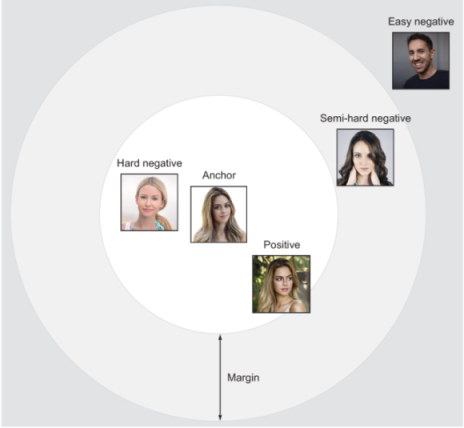
Figure 10.14 Margin: grading triplets into hard, semi-hard, and easy. This illustration (in the context of face recognition) is for an anchor and a corresponding negative sample. Therefore, negative samples that are closer to the anchor are hard.
Figure 10.15 illustrates the hardness of a triplet. Remember that a positive sample is harder if the network (at a training epoch) puts this sample far from its anchor in the embedding space. Similarly, in a plot of distances from the anchor to negative data, the samples closer (less distant) to the anchor are harder. As a reminder, here is the triplet loss function for an anchor (a), positive (p), and negative (n):
ltriplet (a, p, n) = [Dap − Dan + α]+
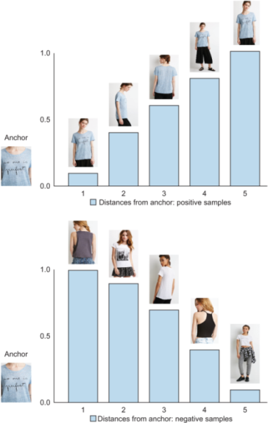
Figure 10.15 Hard-positive and hard-negative data. The plot shows the distances of positive samples (top) and negative samples (bottom) with respect to an anchor (at a particular epoch). The hardness of samples increases as we move from left to right on both plots.
Having explored the concept of hard data and its pitfalls, we will now explore various online triplet mining techniques for our batch. Once a batch (of size PK ) is constructed by the dataloader, there are PK possible anchors. How to find positive and negative data for these anchors is the crux of mining techniques. First we look at two simple and effective online triplet mining techniques: batch all (BA) and batch hard (BH ).
10.4.3 Batch all (BA)
In the context of a batch, batch all (BA ) refers to using all possible and valid triplets; that is, we are not performing any ranking or selection of triplets. In implementation terms, for an anchor, this loss is computed by summing across all possible valid triplets. For a batch size of PK images, since BA selects all triplets, the number of terms updating the triplet loss is PK(K - 1)(K(P - 1)).
Using this approach, all samples (triplets) are equally important; hence this is straightforward to implement. On the other hand, BA can potentially lead to information averaging out. In general, many valid triplets are trivial (at a low loss or non-informative), and only a few are informative. Summing across all valid triplets with equal weights leads to averaging out the contribution of the informative triplets. Hermans et al. [11] experienced this averaging out and reported it in the context of person re-identification.
10.4.4 Batch hard (BH)
As opposed to BA, batch hard (BH ) considers only the hardest data for an anchor. For each possible anchor in a batch, BH computes the loss with exactly one hardest positive data item and one hardest negative data item. Notice that here, the hardness of a datapoint is relative to the anchor. For a batch size of PK images, since BH selects only one positive and one negative per anchor, the number of terms updating the triplet loss is PK (total number of possible anchors).
BH is robust to information averaging out, because trivial (easier) samples are ignored. However, it is potentially difficult to disambiguate with respect to outliers: outliers can creep in due to incorrect annotations, and the model tries hard to converge on them, thereby jeopardizing training quality. In addition, when a not-pretrained network is used prior to using BH, the hardness of a sample (with respect to an anchor) cannot be determined reliably. There is no way to gain this information during training, because the hardest sample is now any random sample, and this can lead to a stall in training. This is reported in [9] and when BH is applied to train a network from scratch in the context of vehicle re-identification in [10].
To visually understand BA and BH, let’s look again at our figure illustrating the distances of the anchor to all positive and negative data (figure 10.16). BA performs no selection and uses all five samples to compute a final loss, whereas BH uses only the hardest available data (ignoring all the rest). Figure 10.17 shows the algorithm outline for computing BH and BA.
![]()
![]()
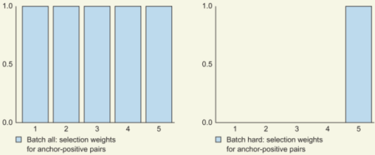
Plot showing selection weights for positive samples with respect to an anchor. For BA, all samples are equally important, while BH gives importance to only the hardest samples (the rest are ignored).

Figure 10.16 Illustration of hard data: distances of positive samples from an anchor (at a particular epoch) (left); distances of negative samples from an anchor (right). BA takes all samples into account, whereas BH takes samples only at the far-right bar (the hardest-positive data for this mini-batch).

Figure 10.17 Algorithm for computing BA and BH
10.4.5 Batch weighted (BW)
BA is a straightforward sampling that weights all samples uniformly. This uniform weight distribution can ignore the contribution of important tough samples, as these samples are typically outnumbered by trivial, easy samples. To mitigate this issue with BA, Ristani et al. [13] employ a batch weighted (BW ) weighting scheme: a sample is weighted based on its distance from the corresponding anchor, thereby giving more importance to informative (harder) samples than trivial samples. Corresponding weights for positive and negative data are shown in table 10.1. Figure 10.18 demonstrates the weighting of samples in this technique.
Table 10.1 Snapshot of various ways to mine good positive xp and negative xn [10]. BS and BW are explored in the upcoming section with examples.
|
|
|||
|
Weights are sampled based on their distance from the anchor. |


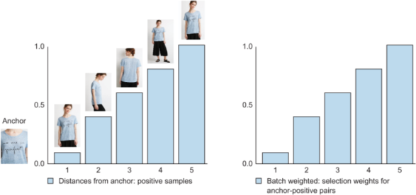
Figure 10.18 BW illustration of selecting positive data for the anchor in the left plot. In this case, all five positive samples are used (as in BA), but a weight-age is assigned to each sample. Unlike BA, which weighs every sample equally, the plot at right weighs each sample in proportion to the corresponding distance from the anchor. This effectively means we are paying more attention to a positive sample that is farther from the anchor (and thus is harder and more informative). Negative data for this anchor is chosen in the same manner, but with reverse weight-age.
10.4.6 Batch sample (BS)
Another sampling technique is batch sample (BS ); it is actively discussed in the implementation page of Hermans el al. [11] and has been used for state-of-the-art vehicle re-identification by Kumar et al. [10]. BS uses the distribution of anchor-to-sample distances to mine2 positive and negative data for an anchor (see figure 10.19). This technique thereby avoids sampling outliers when compared with BH, and it also hopes to determine the most relevant sample as the sampling is done using a distances-to-anchor distribution.

Figure 10.19 BS illustration of selecting a positive data for an anchor. Similarly to BH, the aim is to find one positive data item (for the anchor in the left plot) that is informative and not an outlier. BH would take the hardest data item, which could lead to finding outliers. BS uses the distances as a distribution to mine a sample in a categorical fashion, thereby selecting a sample that is informative and that may not be an outlier. (Note that this is a random multinomial selection; we chose the third sample here just to illustrate the concept.)
Now, let’s unpack these ideas by working through a project and diving deeper into the machinery required for training and testing a CNN for an embedding.
10.5 Project: Train an embedding network
In this project, we put our concepts into practice by building an image-based query retrieval system. We chose two problems that are popular in the visual embedding literature and have been actively studied to find better solutions:
-
Shopping dilemma --Find me apparel that is similar to a query item.
-
Re-identification --Find similar cars in a database; that is, identify a car from different viewpoints (cameras).
Regardless of the tasks, the training, inference, and evaluation processes are the same. Here are some of the ingredients for successfully training an embedding network:
-
Training set --We follow a supervised learning approach with annotations underlining the inherent similarity measure. The dataset can be organized into a set of folders where each folder determines the identity/category of the images. The objective is that images belonging to the same category are kept closer to one another in the embedding space, and vice versa for images in separate categories.
-
Testing set --The test set is usually split into two sets: query and gallery (often, academic papers refer to the gallery set as the test set). The query set consists of images that are used as queries. Each image in the gallery set is ranked (retrieved) against every query image. If the embedding is learned perfectly, the top-ranked (retrieved) items for a query all belong to the same class.
-
Distance metric --To express similarity between two images in an embedding space, we use the Euclidean (L2) distance between the respective embeddings.
-
Evaluation --To quantitatively evaluate a trained model, we use the top-k accuracy and mean average precision (mAP) metrics explained in chapters 4 and 7, respectively. For each object in a query set, the aim is to retrieve a similar identity from the test set (gallery set). AP(q) for a query image q is defined as
where P(k) represents precision at rank k, Ngt(q) is the total number of true retrievals for q, and δk is a Boolean indicator function. So, its value is 1 when the matching of query image q to a test image is correct at rank £ k. Correct retrieval means the ground-truth label for both query and test is the same.
The mAP is then computed as an average over all query images
where Q is the total number of query images. The following sections look at both tasks in more detail.


10.5.1 Fashion: Get me items similar to this
The first task is to determine whether two images taken in a shop belong to the same clothing item. Shopping objects (clothes, shoes) related to fashion are key areas of visual search in industrial applications such as image-recommendation engines that recommend products similar to what a shopper is looking for. Liu et al. [3] introduced one of the largest datasets (DeepFashion) for shopping image-retrieval tasks. This benchmark contains 54,642 images of 11,735 clothing items from the popular Forever 21 catalog. The dataset comprises 25,000 training images and about 26,000 test images, split across query and gallery sets; figure 10.20 shows sample images.

Figure 10.20 Each row indicates a particular category and corresponding similar images. A perfectly learned embedding would make embeddings of images in each row closer to each other than any two images across columns (which belong to different apparel categories). (Images in this figure are taken from the DeepFashion dataset [3].)
10.5.2 Vehicle re-identification
Re-identification is the task of matching the appearance of objects in and across camera networks. A usual pipeline here involves a user seeking all instances of a query object’s presence in all cameras within a network. For example, a traffic regulator may be looking for a particular car across a city-wide camera network. Other examples are person and face re-identification, which are mainstays in security and biometrics.
This task uses the famous VeRi dataset from Liu et al. [14, 36]. This dataset encompasses 40,000 bounding-box annotations of 776 cars (identities) across 20 cameras in traffic surveillance scenes; figure 10.21 shows sample images. Each vehicle is captured by 2 to 18 cameras in various viewpoints and varying illuminations. Notably, the viewpoints are not restricted to only front/rear but also include side views, thereby making this a challenging dataset. The annotations include make and model of vehicles, color, and inter-camera relations and trajectory information.

Figure 10.21 Each row indicates a vehicle class. Similar to the apparel task, the goal (training an embedding CNN) here is to push the embeddings of the same class closer than the embeddings of different classes. (Images in this figure are from the VeRi dataset [14].)
We will use only category (or identity) level annotations; we will not use attributes like make, model, and spatio-temporal location. Incorporating more information during training could help gain accuracy, but this is beyond the scope of this chapter. However, the last part of the chapter references some cool new developments in incorporating multi-source information for learning embeddings.
10.5.3 Implementation
This project uses the GitHub codebase of triplet learning (https://github.com/VisualComputingInstitute/triplet-reid/tree/sampling) attached to [11]. Dataset preprocessing and a summary of steps are available with the book’s downloadable code; go to the project’s Jupyter notebook to follow along with a step-by-step tutorial of the project implementation. TensorFlow users are encouraged to look at the blog post “Triplet Loss and Online Triplet Mining in TensorFlow” by Olivier Moindrot (https://omoindrot.github.io/triplet-loss) to understand various ways of implementing triplet loss.
Training a deep CNN involves several key hyperparameters, and we briefly discuss them here. Following is a summary of the hyperparameters we set for this project:
-
Meta-architecture : We use Mobilenet-v1 [16], which has 569 million MACs and measures the number of fused multiplication and addition operations. This architecture has 4.24 million parameters and achieves a top-1 accuracy of 70.9% on ImageNet’s image classification benchmark, with input image size of 224 × 224.
-
Optimizer : We use the Adam optimizer [17] with default hyperparameters (ε = 10-3, β 1 = 0.9, β 2 = 0.999). Initial learning rate is set to 0.0003.
-
Data augmentation is performed in an online fashion using a standard image-flip operation.
-
Batch size is 18 (P ) randomly sampled identities, with 4 (K ) samples per identity, for a total of 18 × 4 samples in a batch.
-
Margin : The authors replaced the hinge loss [.]+ with a smooth variation called softplus: ln(1 + .). Our experiments also apply softplus instead of using a hard margin.
-
Embedding dimension corresponds to the dimension of the last fully connected layer. We fix this to 128 units for all experiments. Using a lower embedding size is helpful for computational efficiency.
DEFINITION In computing, the multiply-accumulate operation is a common step that computes the product of two numbers and adds that product to an accumulator. The hardware unit that performs the operation is known as a multiplier-accumulator (MAC, or MAC unit ); the operation itself is also often referred to as MAC or a MAC operation.
10.5.4 Testing a trained model
To test a trained model, each dataset presents two files: a query set and a gallery set. These sets can be used to compute the evaluation metrics mentioned earlier: mAP and top-k accuracy. While evaluation metrics are a good summary, we also look at the results visually. To this end, we take random images in a query set and find (plot) the top-k retrievals from the gallery set. The following subsections show quantitative and qualitative results of using various mining techniques from this chapter.
Task 1: In-shop retrieval
Let’s look at sample retrievals from the learned embeddings in figure 10.22. The results look visually pleasing: the top retrievals are from the same class as the query. The network does reasonably well at inferring different views of the same query in the top ranks.
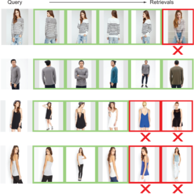
Figure 10.22 Sample retrievals from the fashion dataset using various embedding approaches. Each row indicates the query image and top-5 retrievals for this query image. An x indicates an incorrect retrieval.
Table 10.2 outlines the performance of triplet loss under various sampling scenarios. BW outperforms all other sampling approaches. Top-1 accuracy is quite good in this case: we were able to retrieve the same class of fashion object in the very first retrieval, with accuracy over 87%. Notice that with the evaluation setup, the top-k accuracy for k > 1 is higher (monotonically).
Table 10.2 Performance of various sampling approaches on the in-shop retrieval task
Our results compare favorably with the state-of-the-art results. Using attention-based ensemble (ABE) [18], a diverse set of ensembles are trained that attend to parts of the image. Boosting independent embeddings robustly (BIER) [19] trains an ensemble of metric CNNs with a shared feature representation as an online gradient boosting problem. Noticeably, this ensemble framework does not introduce any additional parameters (and works with any differential loss).
Task 2: Vehicle re-identification
Kumar et al. [12] recently performed an exhaustive evaluation of the sampling variants for optimizing triplet loss. The results are summarized in table 10.3 with comparisons from several state-of-the-art approaches. Noticeably, the authors perform favorably compared to state-of-the-art approaches without using any other information sources, such as spatio-temporal distances and attributes. Qualitative results are shown in figure 10.23, demonstrating the robustness of embeddings with respect to the viewpoints. Notice that the retrieval has the desired property of being viewpoint-invariant, as different views of the same vehicle are retrieved into top-5 ranks.
Table 10.3 Comparison of various proposed approaches on the VeRi dataset. An asterisk (*) indicates the usage of spatio-temporal information.

Figure 10.23 Sample retrievals on the VeRi dataset using various embedding approaches. Each row indicates a query image and the top-5 retrievals for it. An x indicates an incorrect retrieval.
To gauge the pros and cons of various approaches in the literature, let’s conceptually examine the competing approaches in vehicle re-identification:
-
Kanaci et al. [26] proposed cross-level vehicle re-identification (CLVR ) on the basis of using classification loss with model labels (see figure 10.24) to train a fine-grained vehicle categorization network. This setup is similar to the one we saw in section 10.3.2 and figure 10.9. The authors did not perform an evaluation on the VeRi dataset. You are encouraged to refer to this paper to understand the performance on other vehicle re-identification datasets.
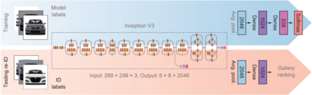
Figure 10.24 Cross-level vehicle re-identification (CLVR). (Source: [24].)
-
Group-sensitive triplet embedding (GSTE ) by Bai et al. [20] is a novel training process that clusters intra-class variations using K-Means. This helps with more guided training at the expense of an additional parameter, K-Means clustering.
-
Pose aware multi-task learning (PAMTRI ) by Zheng et al. [23] trains a network for embedding in a multi-task regime using keypoint annotations in conjunction with synthetic data (thereby tackling keypoint annotation requirements). PAMTRI (All) achieves the best results on this dataset. PAMTRI (RS) uses a mix of real and synthetic data for learning embedding, and PAMTRI (All) additionally uses vehicle keypoints and attributes in a multi-task learning framework.
-
Adaptive attention for vehicle re-identification (AAVER ) by Khorramshahi et al. [25] is a recent work wherein the authors construct a dual-path network for extracting global and local features. These are then concatenated to form a final embedding. The proposed embedding loss is minimized using identity and keypoint orientation annotations.
-
A training procedure for viewpoint attentive multi-view inference (VAMI ) by Zhou et al. [21] includes a generative adversarial network (GAN) and multi-view attention learning. The authors’ conjecture that being able to synthesize (generate using GAN) multiple viewpoint views would help learn a better final embedding.
-
With Path-LSTM, Shen et al. [22] employ a generation of several path proposals for their spatio-temporal regularization and require an additional LSTM to rank these proposals.
-
Kanaci et al. [24] proposed multi-scale vehicle representation (MSVR ) for re-identification by exploiting a pyramid-based DL method. MSVR learns vehicle re-identification sensitive feature representations from an image pyramid with a network architecture of multiple branches, all of which are optimized concurrently.
A snapshot summary of these approaches with respect to the key hyperparameters is summarized in table 10.4.
Table 10.4 Summary of some important hyperparameters and labeling used during training
Usually, license plates are a global unique identifier. However, with the standard installation of traffic cameras, license plates are difficult to extract; hence, visual-based features are required for vehicle re-identification. If two cars are of the same make, model, and color, then visual features cannot disambiguate them (unless there are some distinctive marks such as text or scratches). In these tough scenarios, only spatio-temporal information (like GPS information) can help. To learn more, you are encouraged to look into recent proposed datasets by Tang et al. [27].
10.6 Pushing the boundaries of current accuracy
Deep learning is an evolving field, and novel approaches to training are being introduced every day. This section provides ideas for improving the current level of embeddings and some recently introduced tips and tricks to train a deep CNN:
-
Re-ranking --After obtaining an initial ranking of gallery images (to an input query image), re-ranking uses a post-processing step with the aim of improving the ranking of relevant images. This is a powerful, widely used step in many re-identification and information-retrieval systems.
A popular approach in re-identification is by Zhong et al. [28] (see figure 10.25). Given a probe p and a gallery set, the appearance feature (embedding) and k-reciprocal feature are extracted for each person. The original distance d and Jaccard distance Jd are calculated for each pair of a probe person and a gallery person. The final distance is then computed as the combination of d and Jd and used to obtain the proposed ranking list.
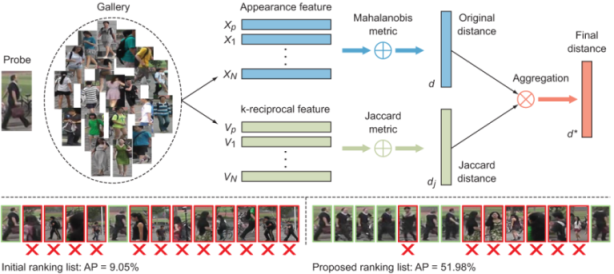
Figure 10.25 Re-ranking proposal by Zhong et al. (Source: [28].)
A recent work in vehicle re-identification, AAVER [25] boosts mAP accuracy by 5% by post-processing using re-ranking.
DEFINITION The Jaccard distance is computed among two sets of data and expresses the intersection over the union of the two sets.
-
Tips and tricks --Luo et al. [29] demonstrated powerful baseline performance on the task of person re-identification. The authors follow the same batch construction from Hermans et al. [11] (studied in this chapter) and use tricks for data augmentation, warm-up learning rate, and label smoothing, to name a few. Noticeably, the authors perform favorably compared to many state-of-the-art methods. You are encouraged to apply these general tricks for training a CNN for any recognition-related tasks.
DEFINITIONS The warm-up learning rate refers to a strategy with a learning rate scheduler that modulates the learning rate linearly with respect to a predefined number of initial training epochs. Label smoothing modulates the cross-entropy loss so the resulting loss is less overconfident on the training set, thereby helping with model generalization and preventing overfitting. This is particularly useful in small-scale datasets.
-
Attention --In this chapter, we focused on learning embedding in a global fashion: that is, we did not explicitly guide the network to attend to, for example, discriminative parts of an object. Some of the prominent works employing attention are Liu et al. [30] and Chen et al. [31]. Employing attention could also help improve the cross-domain performance of a re-identification network, as demonstrated in [32].
-
Guiding training with more information --The state-of-the-art comparisons in table 10.3 briefly touched on works incorporating information from multiple sources: identity, attributes (such as the make and model of a vehicle), and spatio-temporal information (GPS location of each query and gallery image). Ideally, including more information helps obtain higher accuracy. However, this comes at the expense of labeling data with annotations. A reasonable approach for training with a multi-attribute setup is to use multi-task learning (MTL). Often, the loss becomes conflicting; this is resolved by weighting the tasks appropriately (using cross validation). A MTL framework to resolve this conflicting loss scenario using multi-objective optimization is by Sener al. [32].
Some popular works of MTL in the context of face, person, and vehicle categorization are by Ranjan et al. [34], Ling et al. [35], and Tang [23].
Summary
-
Image-retrieval systems require the learning of visual embeddings (a vector space). Any pair of images can be compared using their geometric distance in this embedding space.
-
To learn embeddings using a CNN, there are three popular loss functions: cross-entropy, triplet, and contrastive.
-
Naive training of triplet loss is computationally prohibitive. Hence we use batch-based informative data minings: batch all, batch hard, batch sample, and batch weighted.
References
-
S.Z. Li and A.K. Jain. 2011. Handbook of Face Recognition. Springer Science & Business Media. https://www.springer.com/gp/book/9780857299314.
-
V. Gupta and S. Mallick. 2019. “Face Recognition: An Introduction for Beginners.” Learn OpenCV. April 16, 2019. https://www.learnopencv.com/face-recognition-an-introduction-for-beginners.
-
Z. Liu, P. Luo, S. Qiu, X. Wang, and X. Tang. 2016. “Deepfashion: Powering robust clothes recognition and retrieval with rich annotations.” IEEE Conference on Computer Vision and Pattern Recognition (CVPR). http://mmlab.ie .cuhk.edu.hk/projects/DeepFashion.html.
-
T. Xiao, S. Li, B. Wang, L. Lin, and X. Wang. 2016. “Joint Detection and Identification Feature Learning for Person Search.” http://arxiv.org/abs/1604.01850.
-
Y. Zhai, X. Guo, Y. Lu, and H. Li. 2018. “In Defense of the Classification Loss for Person Re-Identification.” http://arxiv.org/abs/1809.05864.
-
S. Chopra, R. Hadsell, and Y. LeCun. 2005. “Learning a Similarity Metric Discriminatively, with Application to Face Verification.” In 2005 IEEE Computer Society Conference on Computer Vision and Pattern Recognition (CVPR’05 ), 1: 539-46 vol. 1. https://doi.org/10.1109/CVPR.2005.202.
-
C-Y. Wu, R. Manmatha, A.J. Smola, and P. Krähenbühl. 2017. “Sampling Matters in Deep Embedding Learning.” http://arxiv.org/abs/1706.07567.
-
Q. Weinberger and L.K. Saul. 2009. “Distance Metric Learning for Large Margin Nearest Neighbor Classification.” The Journal of Machine Learning Research 10: 207-244. https://papers.nips.cc/paper/2795-distance-metric-learning-for-large-margin-nearest-neighbor-classification.pdf.
-
F. Schroff, D. Kalenichenko, and J. Philbin. 2015. “FaceNet: A Unified Embedding for Face Recognition and Clustering.” In 2015 IEEE Conference on Computer Vision and Pattern Recognition (CVPR ), 815-23. https://ieeexplore.ieee.org/ document/7298682.
-
R. Kumar, E. Weill, F. Aghdasi, and P. Sriram. 2019. “Vehicle Re-Identification: An Efficient Baseline Using Triplet Embedding.” https://arxiv.org/pdf/1901 .01015.pdf.
-
A. Hermans, L. Beyer, and B. Leibe. 2017. “In Defense of the Triplet Loss for Person Re-Identification.” http://arxiv.org/abs/1703.07737.
-
R. Kumar, E. Weill, F. Aghdasi, and P. Sriram. 2020. “A Strong and Efficient Baseline for Vehicle Re-Identification Using Deep Triplet Embedding.” Journal of Artificial Intelligence and Soft Computing Research 10 (1): 27-45. https://content .sciendo.com/view/journals/jaiscr/10/1/article-p27.xml.
-
E. Ristani and C. Tomasi. 2018. “Features for Multi-Target Multi-Camera Tracking and Re-Identification.” http://arxiv.org/abs/1803.10859.
-
X. Liu, W. Liu, T. Mei, and H. Ma. 2018. “PROVID: Progressive and Multimodal Vehicle Reidentification for Large-Scale Urban Surveillance.” IEEE Transactions on Multimedia 20 (3): 645-58. https://doi.org/10.1109/TMM.2017.2751966.
-
J. Deng, W. Dong, R. Socher, L. Li, Kai Li, and Li Fei-Fei. 2009. “ImageNet: A Large-Scale Hierarchical Image Database.” In 2009 IEEE Conference on Computer Vision and Pattern Recognition, 248-55. http://ieeexplore.ieee.org/lpdocs/epic03/ wrapper.htm?arnumber=5206848.
-
A.G. Howard, M. Zhu, B. Chen, D. Kalenichenko, W. Wang, T. Weyand, M. Andreetto, and H. Adam. 2017. “MobileNets: Efficient Convolutional Neural Networks for Mobile Vision Applications.” http://arxiv.org/abs/1704.04861.
-
D.P. Kingma and J. Ba. 2014. “Adam: A Method for Stochastic Optimization.” http://arxiv.org/abs/1412.6980.
-
W. Kim, B. Goyal, K. Chawla, J. Lee, and K. Kwon. 2018. “Attention-based ensemble for deep metric learning.” In 2018 IEEE Conference on Computer Vision and Pattern Recognition (CVPR ), 760-777, https://arxiv.org/abs/1804.00382.
-
M. Opitz, G. Waltner, H. Possegger, and H. Bischof. 2017. “BIER--Boosting Independent Embeddings Robustly.” In 2017 IEEE International Conference on Computer Vision (ICCV ), 5199-5208. https://ieeexplore.ieee.org/document/8237817.
-
Y. Bai, Y. Lou, F. Gao, S. Wang, Y. Wu, and L. Duan. 2018. “Group-Sensitive Triplet Embedding for Vehicle Reidentification.” IEEE Transactions on Multimedia 20 (9): 2385-99. https://ieeexplore.ieee.org/document/8265213.
-
Y. Zhouy and L. Shao. 2018. “Viewpoint-Aware Attentive Multi-View Inference for Vehicle Re-Identification.” In 2018 IEEE/CVF Conference on Computer Vision and Pattern Recognition, 6489-98. https://ieeexplore.ieee.org/document/8578777.
-
Y. Shen, T. Xiao, H. Li, S. Yi, and X. Wang. 2017. “Learning Deep Neural Networks for Vehicle Re-ID with Visual-Spatio-Temporal Path Proposals.” In 2017 IEEE International Conference on Computer Vision (ICCV ), 1918-27. https://ieeexplore .ieee.org/document/8237472.
-
Z. Tang, M. Naphade, S. Birchfield, J. Tremblay, W. Hodge, R. Kumar, S. Wang, and X. Yang. 2019. “PAMTRI: Pose-Aware Multi-Task Learning for Vehicle Re-Identification Using Highly Randomized Synthetic Data.” In Proceedings of the IEEE International Conference on Computer Vision, 211-20. http://openaccess.thecvf .com/content_ICCV_2019/html/Tang_PAMTRI_Pose-Aware_Multi-Task_Learning _for_Vehicle_Re-Identification_Using_Highly_Randomized_ICCV_2019_paper .html.
-
A. Kanacı, X. Zhu, and S. Gong. 2017. “Vehicle Reidentification by Fine-Grained Cross-Level Deep Learning.” In BMVC AMMDS Workshop, 2:772-88. https://arxiv.org/abs/1809.09409.
-
P. Khorramshahi, A. Kumar, N. Peri, S.S. Rambhatla, J.-C. Chen, and R. Chellappa. 2019. “A Dual-Path Model With Adaptive Attention For Vehicle Re-Identification.” http://arxiv.org/abs/1905.03397.
-
A. Kanacı, X. Zhu, and S. Gong. 2017. “Vehicle Reidentification by Fine-Grained Cross-Level Deep Learning.” In BMVC AMMDS Workshop, 2:772-88. http://www .eecs.qmul.ac.uk/~xiatian/papers.
-
Z. Tang, M. Naphade, M.-Y. Liu, X. Yang, S. Birchfield, S. Wang, R. Kumar, D. Anastasiu, and J.-N. Hwang. 2019. “CityFlow: A City-Scale Benchmark for Multi-Target Multi-Camera Vehicle Tracking and Re-Identification.” In 2019 IEEE Conference on Computer Vision and Pattern Recognition (CVPR ). http://arxiv.org/ abs/1903.09254.
-
Z. Zhong, L. Zheng, D. Cao, and S. Li. 2017. “Re-Ranking Person Re-Identification with K-Reciprocal Encoding.” In 2017 IEEE Conference on Computer Vision and Pattern Recognition (CVPR ), 3652-3661, https://arxiv.org/abs/1701.08398.
-
H. Luo, Y. Gu, X. Liao, S. Lai, and W. Jiang. 2019. “Bag of Tricks and A Strong Baseline for Deep Person Re-Identification.” In 2019 IEEE Conference on Computer Vision and Pattern Recognition (CVPR ) Workshops. https://arxiv.org/abs/ 1903.07071.
-
H. Liu, J. Feng, M. Qi, J. Jiang, and S. Yan. 2016. “End-to-End Comparative Attention Networks for Person Re-Identification.” IEEE Transactions on Image Processing 26 (7): 3492-3506. https://arxiv.org/abs/1606.04404.
-
G. Chen, C. Lin, L. Ren, J. Lu, and J. Zhou. 2019. “Self-Critical Attention Learning for Person Re-Identification.” In Proceedings of the IEEE International Conference on Computer Vision, 9637-46. http://openaccess.thecvf.com/content_ICCV_ 2019/html/Chen_Self-Critical_Attention_Learning_for_Person_Re-Identification _ICCV_2019_paper.html.
-
H. Liu, J. Cheng, S. Wang, and W. Wang. 2019. “Attention: A Big Surprise for Cross-Domain Person Re-Identification.” http://arxiv.org/abs/1905.12830.
-
O. Sener and V. Koltun. 2018. “Multi-Task Learning as Multi-Objective Optimization.” In Proceedings of the 32nd International Conference on Neural Information Processing Systems, 525-36. http://dl.acm.org/citation.cfm?id=3326943.3326992.
-
R. Ranjan, S. Sankaranarayanan, C. D. Castillo, and R. Chellappa. 2017. “An All-In-One Convolutional Neural Network for Face Analysis.” In 2017 12th IEEE International Conference on Automatic Face Gesture Recognition (FG 2017 ), 17-24. https://arxiv.org/abs/1611.00851.
-
H. Ling, Z. Wang, P. Li, Y. Shi, J. Chen, and F. Zou. 2019. “Improving Person Re-Identification by Multi-Task Learning.” Neurocomputing 347: 109-118. https:// doi.org/10.1016/j.neucom.2019.01.027.
-
X. Liu, W. Liu, T. Mei, and H. Ma. 2016. “A Deep Learning-Based Approach to Progressive Vehicle Re-Identification for Urban Surveillance.” In Computer Vision - ECCV 2016, 869-84. https://doi.org/10.1007/978-3-319-46475-6_53.
-
B. Amos, B. Ludwiczuk, M. Satyanarayanan, et al. 2016. “Openface: A General-Purpose Face Recognition Library with Mobile Applications.” CMU School of Computer Science 6: 2. http://elijah.cs.cmu.edu/DOCS/CMU-CS-16-118.pdf.
1.In practice, this step gets unwound into two for loops due to host memory limitations.
2.Categorically. For an example in Tensorflow, see http://mng.bz/zjvQ.