
This chapter describes convolutional neural networks (CNNs). CNNs are used everywhere in AI, including image recognition and speech recognition. This chapter will detail the mechanisms of CNNs and how to implement them in Python.
Overall Architecture
First, let's look at the network architecture of CNNs. You can create a CNN by combining layers, much in the same way as the neural networks that we have seen so far. However, CNNs have other layers as well: a convolution layer and a pooling layer. We will look at the details of the convolution and pooling layers in the following sections. This section describes how layers are combined to create a CNN.
In the neural networks that we have seen so far, all the neurons in adjacent layers are connected. These layers are called fully connected layers, and we implemented them as Affine layers. You can use Affine layers to create a neural network consisting of five fully connected layers, for example, as shown in Figure 7.1.
As Figure 7.1 shows, the ReLU layer (or the Sigmoid layer) for the activation function follows the Affine layer in a fully connected neural network. Here, after four pairs of Affine – ReLU layers, comes the Affine layer, which is the fifth layer. And finally, the Softmax layer outputs the final result (probability):
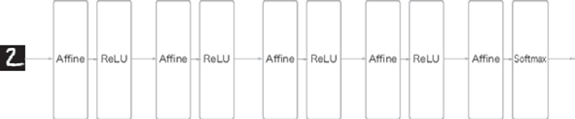
Figure 7.1: Sample network consisting of fully connected layers (Affine layers)
So, what architecture does a CNN have? Figure 7.2 shows a sample CNN:
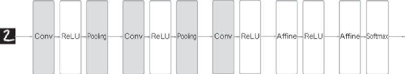
Figure 7.2: Sample CNN – convolution and pooling layers are added (they are shown as gray rectangles)
As shown in Figure 7.2, CNN has additional convolution and pooling layers. In the CNN, layers are connected in the order of Convolution – ReLU – (Pooling) (a pooling layer is sometimes omitted). We can consider the previous Affine – ReLU connection as being replaced with "Convolution – ReLU – (Pooling)."
In the CNN of Figure 7.2, note that the layers near the output are the previous "Affine – ReLU" pairs, while the last output layers are the previous "Affine – Softmax" pairs. This is the structure often seen in an ordinary CNN.
The Convolution Layer
There are some CNN-specific terms, such as padding and stride. The data that flows through each layer in a CNN is data with shape (such as three-dimensional data), unlike in previous fully connected networks. Therefore, you may feel that CNNs are difficult when you learn about them for the first time. Here, we will look at the mechanism of the convolution layer used in CNNs.
Issues with the Fully Connected Layer
The fully connected neural networks that we have seen so far used fully connected layers (Affine layers). In a fully connected layer, all the neurons in the adjacent layer are connected, and the number of outputs can be determined arbitrarily.
The issue with a fully connected layer, though, is that the shape of the data is ignored. For example, when the input data is an image, it usually has a three-dimensional shape, determined by the height, the width, and the channel dimension. However, three-dimensional data must be converted into one-dimensional flat data when it is provided to a fully connected layer. In the previous examples that we used for the MNIST dataset, the input images had the shape of 1, 28, 28 (1 channel, 28 pixels in height, and 28 pixels in width), but the elements were arranged in a line, and the resulting 784 pieces of data were provided to the first Affine layer.
Let's say an image has a three-dimensional shape and that the shape contains important spatial information. Essential patterns to recognize this information may hide in three-dimensional shapes. Spatially close pixels have similar values, the RBG channels are closely related to each other, and the distant pixels are not related. However, a fully connected layer ignores the shape and treats all the input data as equivalent neurons (neurons with the same number of dimensions), so it cannot use the information regarding the shape.
On the other hand, a convolution layer maintains the shape. For images, it receives the input data as three-dimensional data and outputs three-dimensional data to the next layer. Therefore, CNNs can understand data with a shape, such as images, properly.
In a CNN, the input/output data for a convolution layer is sometimes called a feature map. The input data for a convolution layer is called an input feature map, while the output data for a convolution layer is called an output feature map. In this book, input/output data and feature map will be used interchangeably.
Convolution Operations
The processing performed in a convolution layer is called a "convolution operation" and is equivalent to the "filter operation" in image processing. Let's look at example (Figure 7.3) to understand a convolution operation:
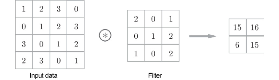
Figure 7.3: Convolution operation – the ⊛ symbol indicates a convolution operation
As shown in Figure 7.3, a convolution operation applies a filter to input data. In this example, the shape of the input data has a height and width, and so does the shape of the filter. When we indicate the shape of the data and filter as (height, width), the input size is (4, 4), the filter size is (3, 3), and the output size is (2, 2) in this example. Some literature uses the word "kernel" for the term "filter."
Now, let's break down the calculation performed in the convolution operation shown in Figure 7.3. Figure 7.4 shows the calculation procedure of the convolution operation.
A convolution operation is applied to the input data while the filter window is shifted at a fixed interval. The window here indicates the gray 3x3 section shown in Figure 7.4. As shown in Figure 7.4, the element of the filter and the corresponding element of the input are multiplied and summed at each location (this calculation is sometimes called a multiply-accumulate operation). The result is stored in the corresponding position of the output. The output of the convolution operation can be obtained by performing this process at all locations.
A fully connected neural network has biases as well as weight parameters. In a CNN, the filter parameters correspond to the previous "weights." It also has biases. The convolution operation of Figure 7.3 shows the stage when a filter was applied. Figure 7.5 shows the processing flow of a convolution operation, including biases:

Figure 7.4: Calculation procedure of a convolution operation
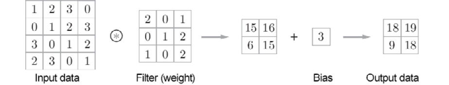
Figure 7.5: Bias in a convolution operation – a fixed value (bias) is added to the element after the filter is applied
As shown in Figure 7.5, a bias term is added to the data after the filter is applied. Here, the bias is always only one (1x1) where one bias exists for the four pieces of data after the filter is applied. This one value is added to all the elements after the filter is applied.
Padding
Before a convolution layer is processed, fixed data (such as 0) is sometimes filled around the input data. This is called padding and is often used in a convolution operation. For example, in Figure 7.6, padding of 1 is applied to the (4, 4) input data. The padding of 1 means filling the circumference with zeros with the width of one pixel:
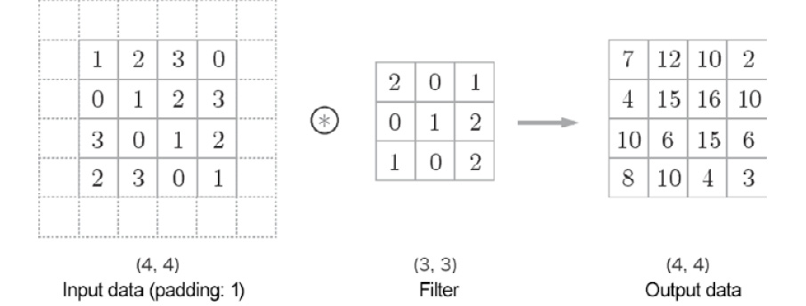
Figure 7.6: Padding in a convolution operation – add zeros around the input data (padding is shown by dashed lines here, and the zeros are omitted)
As shown in Figure 7.6, padding converts the (4, 4) input data into (6, 6) data. After the (3, 3) filter is applied, (4, 4) output data is generated. In this example, the padding of 1 was used. You can set any integer, such as 2 or 3, as the padding value. If the padding value was 2, the size of the input data would be (8, 8). If the padding was 3, the size would be (10, 10).
Note
Padding is used mainly for adjusting the output size. For example, when a (3, 3) filter is applied to (4, 4) input data, the output size is (2, 2). The output size is smaller than the input size by two elements. This causes a problem in deep networks, where convolution operations are repeated many times. If each convolution operation spatially reduces the size, the output size will reach 1 at a certain time, and no more convolution operations will be available. To avoid such a situation, you can use padding. In the previous example, the output size (4, 4) remains the same as the input size (4, 4) when the width of padding is 1. Therefore, you can pass the data of the same spatial size to the next layer after performing a convolution operation.
Stride
The interval of the positions for applying a filter is called a stride. In all previous examples, the stride was 1. When the stride is 2, for example, the interval of the window for applying a filter will be two elements, as shown in Figure 7.7.
In Figure 7.7, a filter is applied to the (7, 7) input data with the stride of 2. When the stride is 2, the output size becomes (3, 3). Thus, the stride specifies the interval for applying a filter.
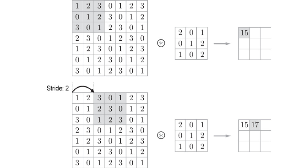
Figure 7.7: Sample convolution operation where the stride is 2
As we have seen so far, the larger the stride, the smaller the output size, and the larger the padding, the larger the output size. How can we represent such relations in equations? Let's see how the output size is calculated based on padding and stride.
Here, the input size is (H, W), the filter size is (FH, FW), the output size is (OH, OW), the padding is P, and the stride is S. In this case, you can calculate the output size with the following equation—that is, equation (7.1):
|
|
(7.1) |
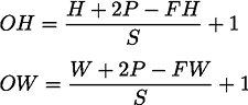
Now, let's use this equation to do some calculations:
- Example 1: Example is shown in Figure 7.6
Input size: (4, 4), padding: 1, stride: 1, filter size: (3, 3):

- Example 2: Example is shown in Figure 7.7
Input size: (7, 7), padding: 0, stride: 2, filter size: (3, 3):

- Example 3
Input size: (28, 31), padding: 2, stride: 3, filter size:(5, 5):

As these examples show, you can calculate the output size by assigning values to equation (7.1). You can only obtain the output size by assignment, but note that you must assign values so that ![]() and
and ![]() in equation (7.1) are divisible. If the output size is not divisible (i.e., the result is a decimal), you must handle that by generating an error. Some deep learning frameworks advance this process without generating an error; for example, they round the value to the nearest integer when it is not divisible.
in equation (7.1) are divisible. If the output size is not divisible (i.e., the result is a decimal), you must handle that by generating an error. Some deep learning frameworks advance this process without generating an error; for example, they round the value to the nearest integer when it is not divisible.
Performing a Convolution Operation on Three-Dimensional Data
The examples we've looked at so far targeted two-dimensional shapes that have a height and a width. For images, we must handle three-dimensional data that has a channel dimension, as well as a height and a width. Here, we will look at an example of a convolution operation on three-dimensional data using the same technique we used in the previous examples.
Figure 7.8 shows an example of convolution operation, while Figure 7.9 shows the calculation procedure. Here, we can see the result of performing a convolution operation on three-dimensional data. You can see that the feature maps have increased in depth (the channel dimension) compared to the two-dimensional data (the example shown in Figure 7.3). If there are multiple feature maps in the channel dimension, a convolution operation using the input data and the filter is performed for each channel, and the results are added to obtain one output:

Figure 7.8: Convolution operation for three-dimensional data
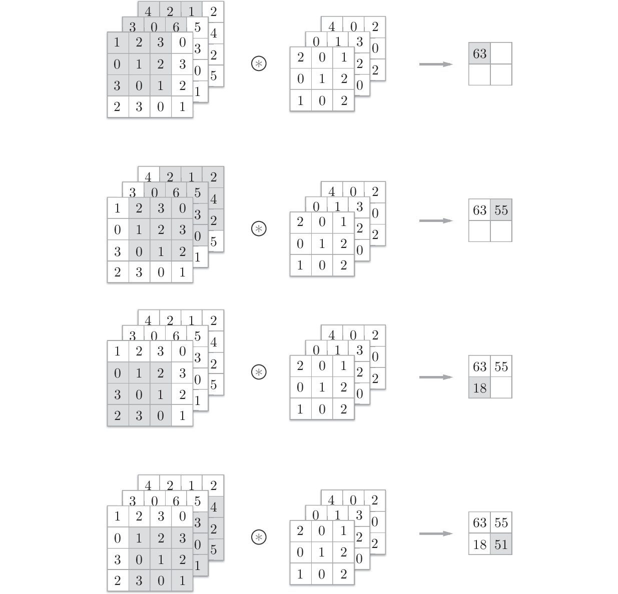
Figure 7.9: Calculation procedure of the convolution operation for three-dimensional data
Note
In a three-dimensional convolution operation, as shown in this example, the input data and the filter must be the same in terms of the number of channels they have. In this example, the number of channels in the input data and the filter are the same; there are three. On the other hand, you can set the filter size to whatever you like. In this example, the filter size is (3, 3). You can set it to any size, such as (2, 2), (1, 1), or (5,5). However, as mentioned earlier, the number of channels must be the same as that of the input data. In this example, there must be three.
Thinking in Blocks
In a three-dimensional convolution operation, you can consider the data and filter as rectangular blocks. A block here is a three-dimensional cuboid, as shown in Figure 7.10. We will represent three-dimensional data as a multidimensional array in the order channel, height, width. So, when the number of channels is C, the height is H, and the width is W for shape, it is represented as (C, H, W). We will represent a filter in the same order so that when the number of channels is C, the height is FH (Filter Height), and the width is FW (Filter Width) for a filter, it is represented as (C, FH, FW):
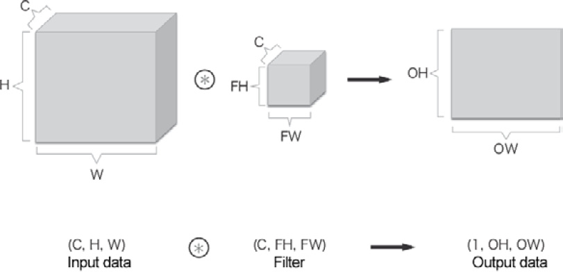
Figure 7.10: Using blocks to consider a convolution operation
In this example, the data's output is one feature map. One feature map means that the size of the output channel is one. So, how can we provide multiple outputs of convolution operations in the channel dimension? To do that, we use multiple filters (weights). Figure 7.11 shows this graphically:

Figure 7.11: Sample convolution operation with multiple filters
As shown in Figure 7.11, when the number of filters applied is FN, the number of output maps generated is also FN. By combining FN maps, you can create a block of the shape (FN, OH, OW). Passing this completed block to the next layer is the process a CNN.
You must also consider the number of filters in a convolution operation. To do that, we will write the filter weight data as four-dimensional data (output_channel, input_channel, height, width). For example, when there are 20 filters with three channels where the size is 5 x 5, it is represented as (20, 3, 5, 5).
A convolution operation has biases (like a fully connected layer). Figure 7.12 shows the example provided in Figure 7.11 when you add biases.
As we can see, each channel has only one bias data. Here, the shape of the bias is (FN, 1, 1), while the shape of the filter output is (FN, OH, OW). Adding these two blocks adds the same bias value to each channel in the filter output result, (FN, OH, OW). NumPy's broadcasting facilitates blocks of different shapes (please refer to Broadcasting section in Chapter 1, Introduction to Python):

Figure 7.12: Process flow of a convolution operation (the bias term is also added)
Batch Processing
Input data is processed in batches in neural network processing. The implementations we've looked at so far for fully connected neural networks have supported batch processing, which enables more efficient processing and supports mini-batches in the training process.
We can also support batch processing in a convolution operation by storing the data that flows through each layer as four-dimensional data. Specifically, the data is stored in the order (batch_num, channel, height, width). For example, when the processing shown in Figure 7.12 is conducted for N data in batches, the shape of the data becomes as follows.
In the data flow for batch processing shown here, the dimensions for the batches are added at the beginning of each piece of data. Thus, the data passes each layer as four-dimensional data. Please note that four-dimensional data that flows in the network indicates that a convolution operation is performed for N data; that is, N processes are conducted at one time:

Figure 7.13: Process flow of a convolution operation (batch processing)
The Pooling Layer
A pooling operation makes the space of the height and width smaller. As shown in Figure 7.14, it converts a 2 x 2 area into one element to reduce the space's size:
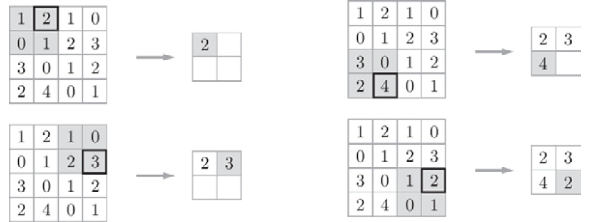
Figure 7.14: Procedure of max pooling
This example shows this procedure when 2 x 2 max-pooling is conducted with a stride of 2. "Max pooling" takes the maximum value of a region, while "2 x 2" indicates the size of the target region. As we can see, it takes the maximum element in a 2 x 2 region. The stride is 2 in this example, so the 2 x 2 window moves by two elements at one time. Generally, the same value is used for the pooling window size and the stride. For example, the stride is 3 for a 3 x 3 window, and the stride is 4 for a 4 x 4 window.
Note
In addition to max pooling, average pooling can also be used. Max pooling takes the maximum value in the target region, while average pooling averages the values in the target region. In image recognition, max pooling is mainly used. Therefore, a "pooling layer" in this book indicates max pooling.
Characteristics of a Pooling Layer
A pooling layer has various characteristics, described below.
There are no parameters to learn
Unlike a convolution layer, a pooling layer has no parameters to learn. Pooling has no parameters to learn because it only takes the maximum value (or averages the values) in the target region.
The number of channels does not change
In pooling, the number of channels in the output data is the same as that in the input data. As shown in Figure 7.15, this calculation is performed independently for each channel:
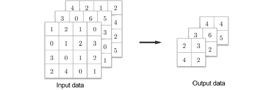
Figure 7.15: Pooling does not change the number of channels
It is robust to a tiny position change
Pooling returns the same result, even when the input data is shifted slightly. Therefore, it is robust to a tiny shift of input data. For example, in 3 x 3 pooling, pooling absorbs the shift of input data, as shown in Figure 7.16:
Figure 7.16: Even when the input data is shifted by one element in terms of width, the output is the same (it may not be the same, depending on the data)
Implementing the Convolution and Pooling Layers
So far, we have seen convolution and pooling layers in detail. In this section, we will implement these two layers in Python. As described in Chapter 5, Backpropagation, the class that will be implemented here also provides forward and backward methods so that it can be used as a module.
You may feel that implementing convolution and pooling layers is complicated, but you can implement them easily if you use a certain "trick." This section describes this trick and makes the task at hand easy. Then, we will implement a convolution layer.
Four-Dimensional Arrays
As described earlier, four-dimensional data flows in each layer in a CNN. For example, when the shape of the data is (10, 1, 28, 28), it indicates that ten pieces of data with a height of 28, width of 28, and 1 channel exist. You can implement this in Python as follows:
>>> x = np.random.rand(10, 1, 28, 28) # Generate data randomly
>>> x.shape
(10, 1, 28, 28)
To access the first piece of data, you can write x[0] ( the index begins at 0 in Python). Similarly, you can write x[1] to access the second piece of data:
>>> x[0].shape # (1, 28, 28)
>>> x[1].shape # (1, 28, 28)
To access the spatial data in the first channel of the first piece of data, you can write the following:
>>> x[0, 0] # or x[0][0]
You can handle four-dimensional data in this way in a CNN. Therefore, implementing a convolution operation may be complicated. However, a "trick" called im2col makes this task easy.
Expansion by im2col
To implement a convolution operation, you normally need to nest for statements several times. Such an implementation is slightly troublesome and for statements in NumPy slow down the processing speed (in NumPy, it is desirable that you do not use any for statements to access elements). Here, we will not use any for statements. Instead, we will use a simple function called im2col for a simple implementation.
The im2col function expands input data conveniently for a filter (weight). As shown in Figure 7.17, im2col converts three-dimensional input data into a two-dimensional matrix (to be exact, it converts four-dimensional data, including the number of batches, into two-dimensional data).
im2col expands the input data conveniently for a filter (weight). Specifically, it expands the area that a filter will be applied to in the input data (a three-dimensional block) into a row, as shown in Figure 7.18. im2col expands all the locations to apply a filter to.
In Figure 7.18, a large stride is used so that the filter areas do not overlap. This is done for visibility reasons. In actual convolution operations, the filter areas will overlap in most cases, in which case, the number of elements after expansion by im2col will be larger than that in the original block. Therefore, an implementation using im2col has the disadvantage of consuming more memory than usual. However, putting data into a large matrix is beneficial to perform calculations with a computer. For example, matrix calculation libraries (linear algebra libraries) highly optimize matrix calculations so that they can multiply large matrices quickly. Therefore, you can use a linear algebra library effectively by converting input data into a matrix:
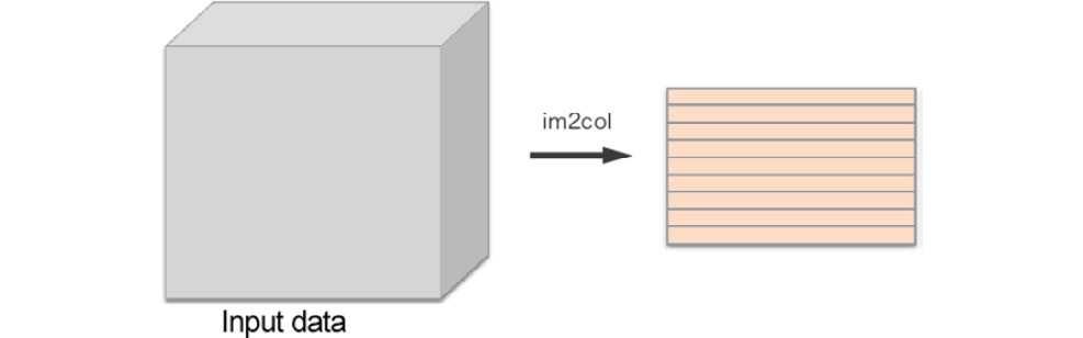
Figure 7.17: Overview of im2col
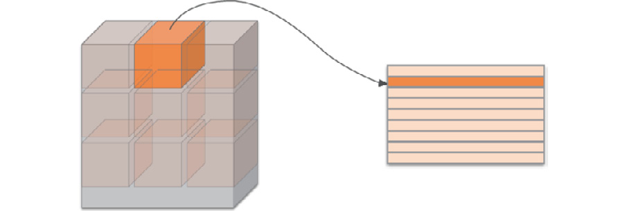
Figure 7.18: Expanding the filter target area from the beginning in a row
Note
The name im2col is an abbreviation of "image to column," meaning the conversion of images into matrices. Deep learning frameworks such as Caffe and Chainer provide the im2col function, which is used to implement a convolution layer.
After using im2col to expand input data, all you have to do is expand the filter (weight) for the convolution layer into a row and multiply the two matrices (see Figure 7.19). This process is almost the same as that of a fully connected Affine layer:
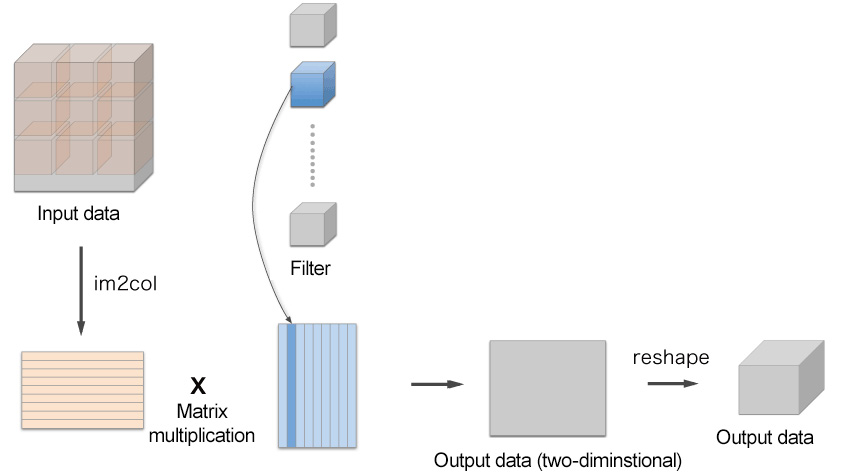
Figure 7.19: Details of filtering in a convolution operation – expand the filter into a column and multiply the matrix by the data expanded by im2col. Lastly, reshape the result of the size of the output data.
As shown in Figure 7.19, the output of using the im2col function is a two-dimensional matrix. You must transform two-dimensional output data into an appropriate shape because a CNN stores data as four-dimensional arrays. The next section covers the flow of implementing a convolution layer.
Implementing a Convolution Layer
This book uses the im2col function, and we will use it as a black box without considering its implementation. The im2col implementation is located at common/util.py. It is a simple function that is about 10 lines in length. Please refer to it if you are interested.
This im2col function has the following interface:
im2col (input_data, filter_h, filter_w, stride=1, pad=0)
- input_data: Input data that consists of arrays of four dimensions (amount of data, channel, height, breadth)
- filter_h: Height of the filter
- filter_w: Width of the filter
- stride: Stride
- pad: Padding
The im2col function considers the "filter size," "stride," and "padding" to expand input data into a two-dimensional array, as follows:
import sys, os
sys.path.append(os.pardir)
from common.util import im2col
x1 = np.random.rand(1, 3, 7, 7)
col1 = im2col(x1, 5, 5, stride=1, pad=0)
print(col1.shape) # (9, 75)
x2 = np.random.rand(10, 3, 7, 7)
col2 = im2col(x2, 5, 5, stride=1, pad=0)
print(col2.shape) # (90, 75)
The preceding code shows two examples. The first one uses 7x7 data with a batch size of 1, where the number of channels is 3. The second one uses data of the same shape with a batch size of 10. When we use the im2col function, the number of elements in the second dimension is 75 in both cases. This is the total number of elements in the filter (3 channels, size 5x5). When the batch size is 1, the result from im2col is (9, 75) in size. On the other hand, it is (90, 75) in the second example because the batch size is 10. It can store 10 times as much data.
Now, we will use im2col to implement a convolution layer as a class called Convolution:
class Convolution:
def __init__(self, W, b, stride=1, pad=0):
self.W = W
self.b = b
self.stride = stride
self.pad = pad
def forward(self, x):
FN, C, FH, FW = self.W.shape
N, C, H, W = x.shape
out_h = int(1 + (H + 2*self.pad - FH) / self.stride)
out_w = int(1 + (W + 2*self.pad - FW) / self.stride)
col = im2col(x, FH, FW, self.stride, self.pad)
col_W = self.W.reshape(FN, -1).T # Expand the filter
out = np.dot(col, col_W) + self.b
out = out.reshape(N, out_h, out_w, -1).transpose(0, 3, 1, 2)
return out
The initialization method of the convolution layer takes the filter (weight), bias, stride, and padding as arguments. The filter is four-dimensional, (FN, C, FH, and FW). FN stands for filter number (number of filters), C stands for a channel, FH stands for filter height, and FW stands for filter width.
In the implementation of a convolution layer, an important section has been shown in bold. Here, im2col is used to expand the input data, while reshape is used to expand the filter into a two-dimensional array. The expanded matrices are multiplied.
The section of code that expands the filter (the section in bold in the preceding code) expands the block of each filter into one line, as shown in Figure 7.19. Here, -1 is specified as reshape (FN, -1), which is one of the convenient features of reshape. When -1 is specified for reshape, the number of elements is adjusted so that it matches the number of elements in a multidimensional array. For example, an array with the shape of (10, 3, 5, 5) has 750 elements in total. When reshape(10, -1) is specified here, it is reshaped into an array with the shape of (10, 75).
The forward function adjusts the output size appropriately at the end. NumPy's transpose function is used there. The transpose function changes the order of axes in a multidimensional array. As shown in Figure 7.20, you can specify the order of indices (numbers) that starts at 0 to change the order of axes.
Thus, you can implement the forward process of a convolution layer in almost the same way as a fully connected Affine layer by using im2col for expansion (see Implementing the Affine and Softmax Layers section in Chapter 5, Backpropagation ). Next, we will implement backward propagation in the convolution layer. Note that backward propagation in the convolution layer must do the reverse of im2col. This is handled by the col2im function, which is provided in this book (located at common/util.py). Except for when col2im is used, you can implement backward propagation in the convolution layer in the same way as the Affine layer. The implementation of backward propagation in the convolution layer is located at common/layer.py.

Figure 7.20: Using NumPy's transpose to change the order of the axes – specifying the indices (numbers) to change the order of axes
Implementing a Pooling Layer
You can use im2col to expand the input data when implementing a pooling layer, as in the case of a convolution layer. What is different is that pooling is independent of the channel dimension, unlike a convolution layer. As shown in Figure 7.21, the target pooling area is expanded independently for each channel.
After this expansion, you have only to take the maximum value in each row of the expanded matrix and transform the result into an appropriate shape (Figure 7.22).
This is how the forward process in a pooling layer is implemented. The following shows a sample implementation in Python:
class Pooling:
def __init__(self, pool_h, pool_w, stride=1, pad=0):
self.pool_h = pool_h
self.pool_w = pool_w
self.stride = stride
self.pad = pad
def forward(self, x):
N, C, H, W = x.shape
out_h = int(1 + (H - self.pool_h) / self.stride)
out_w = int(1 + (W - self.pool_w) / self.stride)
# Expansion (1)
col = im2col(x, self.pool_h, self.pool_w, self.stride, self.pad)
col = col.reshape(-1, self.pool_h*self.pool_w)
# Maximum value (2)
out = np.max(col, axis=1)
# Reshape (3)
out = out.reshape(N, out_h, out_w, C).transpose(0, 3, 1, 2)
return out
Figure 7.21: Expanding the target pooling area of the input data (pooling of 2x2)
As shown in Figure 7.22, there are three steps when it comes to implementing a pooling layer:
- Expand the input data.
- Take the maximum value in each row.
- Reshape the output appropriately.
The implementation of each step is simple and is only one or two lines in length:

Figure 7.22: Flow of implementation of a pooling layer – the maximum elements in the pooling area are shown in gray
Note
You can use NumPy's np.max method to take the maximum value. By specifying the axis argument in np.max, you can take the maximum value along the specified axis. For example, np.max(x, axis=1) returns the maximum value of x on each axis of the first dimension.
That's all for the forward process in a pooling layer. As shown here, after expanding the input data into a shape that's suitable for pooling, subsequent implementations of it are very simple.
For the backward process in a pooling layer, backward propagation of max (used in the implementation of the ReLU layer in the ReLU Layer sub-section in Chapter 5, Backpropagation), provides more information on this. The implementation of a pooling layer is located at common/layer.py.
Implementing a CNN
So far, we have implemented convolution and pooling layers. Now, we will combine these layers to create a CNN that recognizes handwritten digits and implement it, as shown in Figure 7.23.
As shown in Figure 7.23, the network consists of "Convolution – ReLU – Pooling – Affine – ReLU – Affine – Softmax" layers. We will implement this as a class named SimpleConvNet:
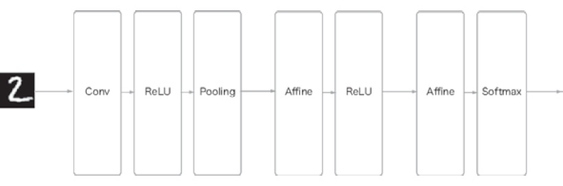
Figure 7.23: Network configuration of a simple CNN
Now, let's look at the initialization of SimpleConvNet (__init__). It takes the following arguments:
- input_dim: Dimensions of the input data (channel, height, width).
- conv_param: Hyperparameters of the convolution layer (dictionary). The following are the dictionary keys:
- filter_num: Number of filters
- filter_size: Size of the filter
- stride: Stride
- pad: Padding
- hidden_size: Number of neurons in the hidden layer (fully connected)
- output_size: Number of neurons in the output layer (fully connected)
- weight_init_std: Standard deviation of the weights at initialization
Here, the hyperparameters of the convolution layer are provided as a dictionary called conv_param. We assume that the required hyperparameter values are stored using {'filter_num':30, 'filter_size':5, 'pad':0, 'stride':1}.
The implementation of the initialization of SimpleConvNet is a little long, so here it's divided into three parts to make this easier to follow. The following code shows the first part of the initialization process:
class SimpleConvNet:
def __init__(self, input_dim=(1, 28, 28),
conv_param={'filter_num':30, 'filter_size':5,
'pad':0, 'stride':1},
hidden_size=100, output_size=10, weight_init_std=0.01):
filter_num = conv_param['filter_num']
filter_size = conv_param['filter_size']
filter_pad = conv_param['pad']
filter_stride = conv_param['stride']
input_size = input_dim[1]
conv_output_size = (input_size - filter_size + 2*filter_pad) /
filter_stride + 1
pool_output_size = int(filter_num * (conv_output_size/2) *(conv_output_size/2))
Here, the hyperparameters of the convolution layer that are provided by the initialization argument are taken out of the dictionary (so that we can use them later). Then, the output size of the convolution layer is calculated. The following code initializes the weight parameters:
self.params = {}
self.params['W1'] = weight_init_std *
np.random.randn(filter_num, input_dim[0],
filter_size, filter_size)
self.params['b1'] = np.zeros(filter_num)
self.params['W2'] = weight_init_std *
np.random.randn(pool_output_size,hidden_size)
self.params['b2'] = np.zeros(hidden_size)
self.params['W3'] = weight_init_std *
np.random.randn(hidden_size, output_size)
self.params['b3'] = np.zeros(output_size)
The parameters required for training are the weights and biases of the first (convolution) layer and the remaining two fully connected layers. The parameters are stored in the instance dictionary variable, params. The W1 key is used for the weight, while the b1 key is used for the bias of the first (convolution) layer. In the same way, the W2 and b2 keys are used for the weight and bias of the second (fully connected) layer and the W3 and b3 keys are used for the weight and bias of the third (fully connected) layer, respectively. Lastly, the required layers are generated, as follows:
self.layers = OrderedDict( )
self.layers['Conv1'] = Convolution(self.params['W1'],
self.params['b1'],
conv_param['stride'],
conv_param['pad'])
self.layers['Relu1'] = Relu( )
self.layers['Pool1'] = Pooling(pool_h=2, pool_w=2, stride=2)
self.layers['Affine1'] = Affine(self.params['W2'],
self.params['b2'])
self.layers['Relu2'] = Relu( )
self.layers['Affine2'] = Affine(self.params['W3'],
self.params['b3'])
self.last_layer = SoftmaxWithLoss( )
Layers are added to the ordered dictionary (OrderedDict) in an appropriate order. Only the last layer, SoftmaxWithLoss, is added to another variable, last-layer.
This is the initialization of SimpleConvNet. After the initialization, you can implement the predict method for predicting and the loss method for calculating the value of the loss function, as follows:
def predict(self, x):
for layer in self.layers.values( ):
x = layer.forward(x)
return x
def loss(self, x, t):
y = self.predict(x)
return self.lastLayer.forward(y, t)
Here, the x argument is the input data and the t argument is the label. The predict method only calls the added layers in order from the top, and passes the result to the next layer. In addition to forward processing in the predict method, the loss method performs forward processing until the last layer, SoftmaxWithLoss.
The following implementation obtains the gradients via backpropagation, as follows:
def gradient(self, x, t):
# forward
self.loss(x, t)
# backward
dout = 1
dout = self.lastLayer.backward(dout)
layers = list(self.layers.values( ))
layers.reverse( )
for layer in layers:
dout = layer.backward(dout)
# Settings
grads = {}
grads['W1'] = self.layers['Conv1'].dW
grads['b1'] = self.layers['Conv1'].db
grads['W2'] = self.layers['Affine1'].dW
grads['b2'] = self.layers['Affine1'].db
grads['W3'] = self.layers['Affine2'].dW
grads['b3'] = self.layers['Affine2'].db
return grads
Backpropagation is used to obtain the gradients of the parameters. To do that, forward propagation and backward propagation are conducted one after the other. Because the forward and backward propagation are implemented properly in each layer, we have only to call them in an appropriate order here. Lastly, the gradient of each weight parameter is stored in the grads dictionary. Thus, you can implement SimpleConvNet.
Now, let's train the SimpleConvNet class using the MNIST dataset. The code for training is almost the same as that described in the Implementing a Training Algorithm section in Chapter 4, Neural Network Training. Therefore, the code won't be shown here (the source code is located at ch07/train_convnet.py).
When SimpleConvNet is used to train the MNIST dataset, the recognition accuracy of the training data is 99.82%, while the recognition accuracy of the test data is 98.96% (the recognition accuracies are slightly different from training to training). 99% is a very high recognition accuracy for the test data for a relatively small network. In the next chapter, we will add layers to create a network where the recognition accuracy of the test data exceeds 99%.
As we have seen here, convolution and pooling layers are indispensable modules in image recognition. A CNN can read the spatial characteristics of images and achieve high accuracy in handwritten digit recognition.
Visualizing a CNN
What does the convolution layer used in a CNN "see"? Here, we will visualize a convolution layer to explore what happens in a CNN.
Visualizing the Weight of the First Layer
Earlier, we conducted simple CNN training for the MNIST dataset. The shape of the weight of the first (convolution) layer was (30, 1, 5, 5). It was 5x5 in size, had 1 channel, and 30 filters. When the filter is 5x5 in size and has 1 channel, it can be visualized as a one-channel gray image. Now, let's show the filters of the convolution layer (the first layer) as images. Here, we will compare the weights before and after training. Figure 7.24 shows the results (the source code is located at ch07/visualize_filter.py):

Figure 7.24: Weight of the first (convolution) layer before and after training. The elements of the weight are real numbers, but they are normalized between 0 and 255 to show the images so that the smallest value is black (0) and the largest value is white (255)
As shown in Figure 7.24, the filters before training are initialized randomly. Black-and-white shades have no pattern. On the other hand, the filters after training are images with a pattern. Some filters have gradations from white to black, while some filters have small areas of color (called "blobs"), which indicates that training provided a pattern to the filters.
The filters with a pattern on the right-hand side of Figure 7.24 "see" edges (boundaries of colors) and blobs. For example, when a filter is white in the left half and black in the right half, it reacts to a vertical edge, as shown in Figure 7.25.
Figure 7.25 shows the results when two learned filters are selected, and convolution processing is performed on the input image. You can see that "filter 1" reacted to a vertical edge and that "filter 2" reacted to a horizontal edge:

Figure 7.25: Filters reacting to horizontal and vertical edges. White pixels appear at a vertical edge in output image 1. Meanwhile, many white pixels appear at a horizontal edge in output image 2.
Thus, you can see that the filters in a convolution layer extract primitive information such as edges and blobs. The CNN that was implemented earlier passes such primitive information to subsequent layers.
Using a Hierarchical Structure to Extract Information
The preceding result comes from the first (convolution) layer. It extracts low-level information such as edges and blobs. So, what type of information does each layer in a CNN with multiple layers extract? Research on visualization in deep learning [(Matthew D. Zeiler and Rob Fergus (2014): Visualizing and Understanding Convolutional Networks. In David Fleet, Tomas Pajdla, Bernt Schiele, & Tinne Tuytelaars, eds. Computer Vision – ECCV 2014. Lecture Notes in Computer Science. Springer International Publishing, 818 – 833) and (A. Mahendran and A. Vedaldi (2015): Understanding deep image representations by inverting them. In the 2015 IEEE Conference on Computer Vision and Pattern Recognition (CVPR). 5188 – 5196. DOI: (http://dx.doi.org/10.1109/CVPR.2015.7299155)] has stated that the deeper a layer, the more abstract the extracted information (to be precise, neurons that react strongly).
Typical CNNs
CNNs of various architectures have been proposed so far. In this section, we will look at two important networks. One is LeNet (Y. Lecun, L. Bottou, Y. Bengio, and P. Haffner (1998): Gradient-based learning applied to document recognition. Proceedings of the IEEE 86, 11 (November 1998), 2278 – 2324. DOI: (http://dx.doi.org/10.1109/5.726791)). It was one of the first CNNs and was first proposed in 1998. The other is AlexNet (Alex Krizhevsky, Ilya Sutskever, and Geoffrey E. Hinton (2012): ImageNet Classification with Deep Convolutional Neural Networks. In F. Pereira, C. J. C. Burges, L. Bottou, & K. Q. Weinberger, eds. Advances in Neural Information Processing Systems 25. Curran Associates, Inc., 1097 – 1105). It was proposed in 2012 and drew attention to deep learning.
LeNet
LeNet is a network for handwritten digit recognition that was proposed in 1998. In the network, a convolution layer and a pooling layer (i.e., a subsampling layer that only "thins out elements") are repeated, and finally, a fully connected layer outputs the result.
There are some differences between LeNet and the "current CNN." One is that there's an activation function. A sigmoid function is used in LeNet, while ReLU is mainly used now. Subsampling is used in the original LeNet to reduce the size of intermediate data, while max pooling is mainly used now:
In this way, there are some differences between LeNet and the "current CNN," but they are not significant. This is surprising when we consider that LeNet was the "first CNN" to be proposed almost 20 years ago.
AlexNet
AlexNet was published nearly 20 years after LeNet was proposed. Although AlexNet created a boom in deep learning, its network architecture hasn't changed much from LeNet:
AlexNet stacks a convolution layer and a pooling layer and outputs the result through a fully connected layer. Its architecture is not much different from LeNet, but there are some differences, as follows:
- ReLU is used as the activation function
- A layer for local normalization called Local Response Normalization (LRN) is used
- Dropout is used (see Dropout sub-section in Chapter 6, Training Techniques)
LeNet and AlexNet are not very different in terms of their network architectures. However, the surrounding environment and computer technologies have advanced greatly. Now, everyone can obtain a large quantity of data, and widespread GPUs that are good at large parallel computing enable massive operations at high speed. Big data and GPUs greatly motivated the development of deep learning.
Note
Many parameters often exist in deep learning (a network with many layers). Many calculations are required for training, and a large quantity of data is required to "satisfy" these parameters. We can say that GPUs and big data cast light on these challenges.
Summary
In this chapter, we learned about CNNs. Specifically, we covered convolution layers and pooling layers (the basic modules that constitute CNNs) in great detail in order to understand them at the implementation level. CNNs are mostly used when looking at data regarding images. Please ensure that you understand the content of this chapter before moving on.
In this chapter, we learned about the following:
- In a CNN, convolution, and pooling layers are added to the previous network, which consists of fully connected layers.
- You can use im2col (a function for expanding images into arrays) to implement convolution and pooling layers simply and efficiently.
- Visualizing a CNN enables you to see how advanced information is extracted as the layer becomes deeper.
- Typical CNNs include LeNet and AlexNet.
- Big data and GPUs contribute significantly to the development of deep learning.