
About
This section is included to assist the students to perform the activities present in the book. It includes detailed steps that are to be performed by the students to complete and achieve the objectives of the activity.
Computational Graph of the Softmax-with-Loss Layer
The following figure is the computational graph of the Softmax-with-Loss layer and obtains backward propagation. We will call the softmax function the Softmax layer, the cross-entropy error the Cross-Entropy Error layer, and the layer where these two are combined the Softmax-with-Loss layer. You can represent the Softmax-with-Loss layer with the computational graph provided in Figure A.1: Entropy:
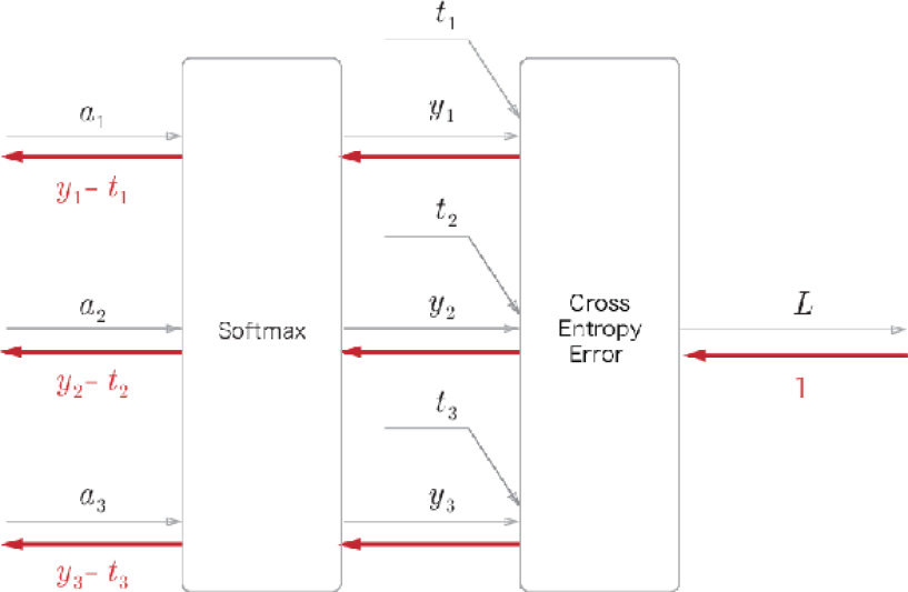
Figure A.1: Computational graph of the Softmax-with-Loss layer
The computational graph shown in Figure A.1 assumes that there is a neural network that classifies three classes. The input from the previous layer is (a1, a2, a3), and the Softmax layer outputs (y1, y2, y3). The label is (t1, t2, t3) and the Cross-Entropy Error layer outputs the loss, L.
This appendix shows that the result of backward propagation of the Softmax-with-Loss layer will be (y1 − t1, y2 − t2, y3 − t3), as shown in Figure A.1.
Forward Propagation
The computational graph shown in Figure A.1 does not show the details of the Softmax layer and the Cross-Entropy Error layer. Here, we will start by describing the details of the two layers.
First, let's look at the Softmax layer. We can represent the softmax function with the following equation:

|
(A.1) |
Therefore, we can show the Softmax layer with the computational graph provided in Figure A.2. Here, S stands for the sum of exponentials, which is the denominator in equation (A.1). The final output is (y1, y2, y3).
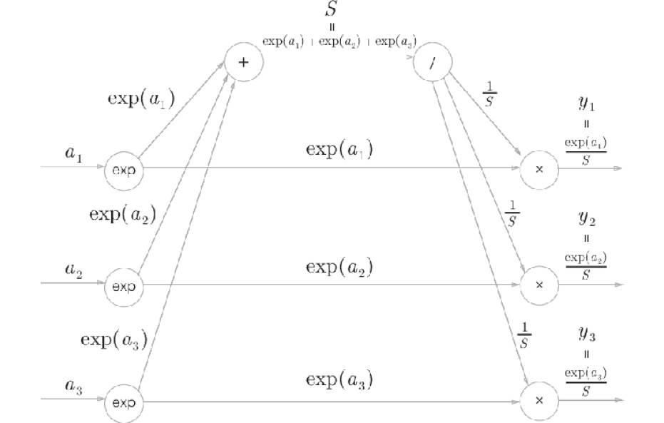
Figure A.2: Computational graph of the Softmax layer (forward propagation only)
Next, let's look at the Cross-Entropy Error layer. The following equation shows the cross-entropy error:

|
(A.2) |
Based on equation (A.2), we can draw the computational graph of the Cross-Entropy Error layer as shown in Figure A.3.
The computational graph shown in Figure A.3 just shows equation (A. 2) as a computational graph. Therefore, I think that there is nothing particularly difficult about this.

Figure A.3: Computational graph of the Cross-Entropy Error layer (forward propagation only)
Now, let's look at backward propagation:
Backward Propagation
First, let's look at backward propagation of the Cross-Entropy Error layer. We can draw backward propagation of the Cross-Entropy Error layer as follows:

Figure A.4: Backward propagation of the Cross-Entropy Error layer
Please note the following to obtain backward propagation of this computational graph:
- The initial value of backward propagation (the rightmost value of backward propagation in Figure A.4) is 1 (because
 ).
). - For backward propagation of the "x" node, the "reversed value" of the input signal for forward propagation multiplied by the derivative from the upper stream is passed downstream.
- For the "+" node, the derivative from the upper stream is passed without changing it.
- The backward propagation of the "log" node observes the following equations:

Based on this, we can obtain backward propagation of the Cross-Entropy Error layer easily. As a result, the value ![]() will be the input to the backward propagation of the Softmax layer.
will be the input to the backward propagation of the Softmax layer.
Next, let's look at backward propagation of the Softmax layer. Because the Softmax layer is a little complicated, I want to check its backward propagation step by step:
Step 1:
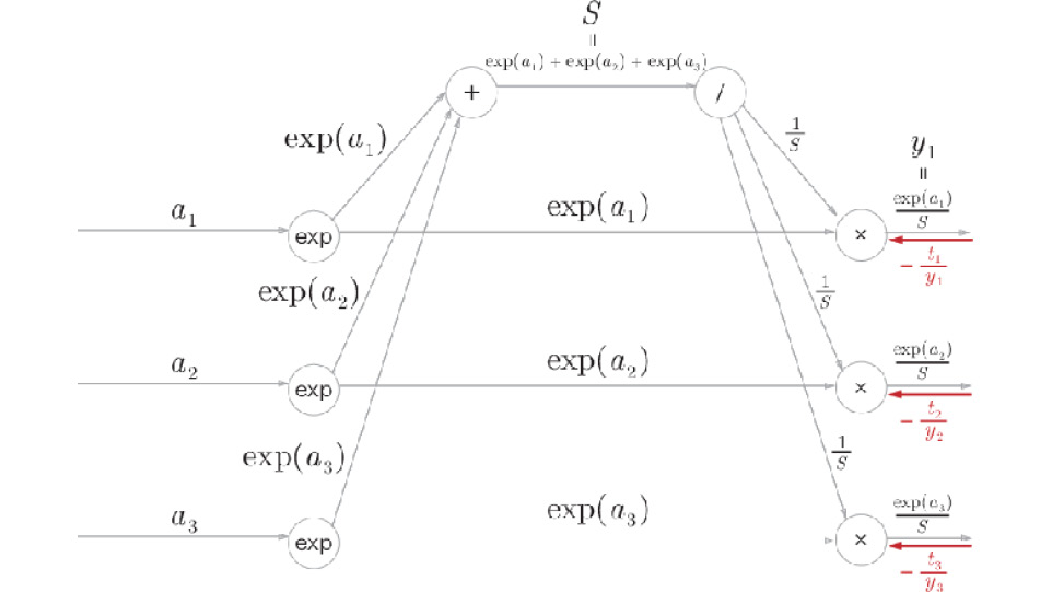
Figure A.5: Step 1
The values of the backward propagation arrive from the previous layer (Cross-Entropy Error layer).
Step 2:
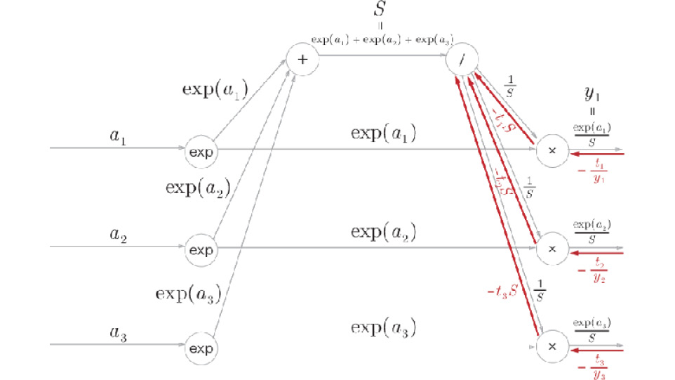
Figure A.6: Step 2
The "x" node "reverses" the values of forward propagation for multiplication. Here, the following calculation is performed:

|
(A.3) |
Step 3:

Figure A.7: Step 3
If the flow branches into multiple values in forward propagation, the separated values are added in backward propagation. Therefore, three separate values of backward propagation, ![]() , are added here. The backward propagation of / is conducted for the added values, resulting in
, are added here. The backward propagation of / is conducted for the added values, resulting in ![]() . Here, (t1, t2, t3) is the label and a "one-hot vector." A one-hot vector means that one of (t1, t2, t3) is 1 and the others are all 0s. Therefore, the sum of (t1, t2, t3) is 1.
. Here, (t1, t2, t3) is the label and a "one-hot vector." A one-hot vector means that one of (t1, t2, t3) is 1 and the others are all 0s. Therefore, the sum of (t1, t2, t3) is 1.
Step 4:
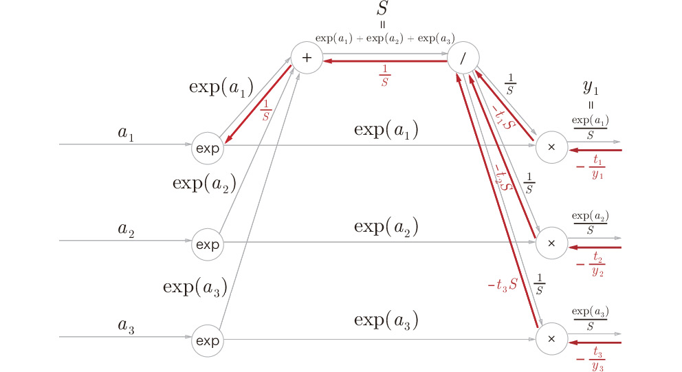
Figure A.8: Step 4
The "+" node only passes the value without changing it.
Step 5:
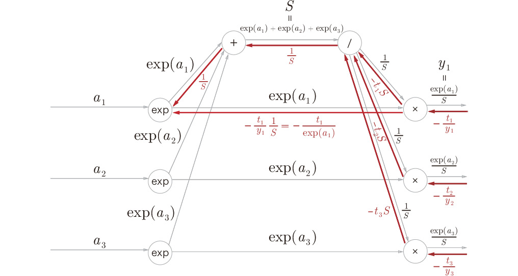
Figure A.9: Step 5
The "x" node "reverses" the values for multiplication. Here, ![]() is used to transform the equation.
is used to transform the equation.
Step 6:

Figure A.10: Step 6
In the "exp" node, the following equations hold true:
|
|
(A.4) |

Thus, the sum of the two separate inputs, which are multiplied by exp(a1), is the backward propagation to obtain. We can write this as ![]() and obtain
and obtain ![]() after transformation. Thus, in the node where the input of forward propagation is
after transformation. Thus, in the node where the input of forward propagation is ![]() , backward propagation is
, backward propagation is ![]() . For
. For ![]() and
and ![]() , we can use the same procedure (the results are
, we can use the same procedure (the results are ![]() and
and ![]() , respectively). With this, it is easy to show that we can achieve the same result even if we want to classify n classes instead of three classes.
, respectively). With this, it is easy to show that we can achieve the same result even if we want to classify n classes instead of three classes.
Summary
Here, the computational graph of the Softmax-with-Loss layer was shown in detail, and its backward propagation was obtained. Figure A.11 shows the complete computational graph of the Softmax-with-Loss layer:

Figure A.11: Computational graph of the Softmax-with-Loss layer
The computational graph shown in Figure A.11 looks complicated. However, if you advance step by step using computational graphs, obtaining derivatives (the procedure of backward propagation) will be much less troublesome. When you encounter a layer that looks complicated (such as the Batch Normalization layer), other than the Softmax-with-Loss layer described here, you can use this procedure. This will be easier to understand in practice rather than only looking at equations.