3 Introduction to Keras and TensorFlow

This chapter is meant to give you everything you need to start doing deep learning in practice. I’ll give you a quick presentation of Keras (https://keras.rstudio.com) and TensorFlow (https://tensorflow.rstudio.com), the R-based deep learning tools that we’ll use throughout the book. You’ll find out how to set up a deep learning workspace with TensorFlow, Keras, and GPU support. Finally, building on top of the first contact you had with Keras and TensorFlow in chapter 2, we’ll review the core components of neural networks and how they translate to the Keras and Tensor-Flow APIs.

By the end of this chapter, you’ll be ready to move on to practical, real-world applications, which will start with chapter 4.

3.1 What’s TensorFlow?

TensorFlow is a free, open source machine learning platform, developed primarily by Google. Much like R itself, the primary purpose of TensorFlow is to enable scientists, engineers, and researchers to manipulate mathematical expressions over numerical tensors. But TensorFlow brings to R the following new capabilities:

• It can automatically compute the gradient of any differentiable expression (as you saw in chapter 2), making it highly suitable for machine learning
• It can run not only on CPUs but also on GPUs and TPUs, which are highly parallel hardware accelerators.
• Computation defined in TensorFlow can be easily distributed across many machines.
• TensorFlow programs can be exported to other runtimes, such as C++, Java-Script (for browser-based applications), or TensorFlow Lite (for applications running on mobile devices or embedded devices). This makes TensorFlow applications easy to deploy in practical settings

It’s important to keep in mind that TensorFlow is much more than a single library. It’s really a platform, home to a vast ecosystem of components, some developed by Google and some developed by third parties. For instance, there’s TF-Agents for reinforcement-learning research, TFX for industry-strength machine learning workflow management, TensorFlow Serving for production deployment, and the TensorFlow Hub repository of pretrained models. Together, these components cover a very wide range of use cases, from cutting-edge research to large-scale production applications.

TensorFlow scales fairly well: for instance, scientists from Oak Ridge National Lab have used it to train a 1.1 exaflops extreme weather forecasting model on the 27,000 GPUs of the IBM Summit supercomputer. Likewise, Google has used TensorFlow to develop very compute-intensive deep learning applications, such as the chess-playing and Go-playing agent AlphaZero. For your own models, if you have the budget, you can realistically hope to scale to around 10 petaflops on a small TPU pod or a large cluster of GPUs rented on Google Cloud or AWS. That would still be around 1% of the peak compute power of the top supercomputer in 2019!

3.2 What’s Keras?

Keras is a deep learning API, built on top of TensorFlow, that provides a convenient way to define and train any kind of deep learning model. Keras was initially developed for research, with the aim of enabling fast deep learning experimentation.

Through TensorFlow, Keras can run on top of different types of hardware (see figure 3.1)—GPU, TPU, or plain CPU—and can be seamlessly scaled to thousands of machines.

Keras is known for prioritizing the developer experience. It’s an API for human beings, not machines. It follows best practices for reducing cognitive load: it offers consistent and simple workflows, it minimizes the number of actions required for common use cases, and it provides clear and actionable feedback upon user error. This makes Keras easy to learn for a beginner and highly productive to use for an expert.

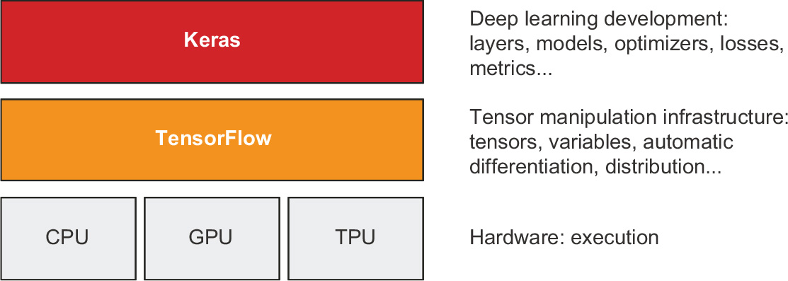
Figure 3.1 Keras and TensorFlow: TensorFlow is a low-level tensor computing platform, and Keras is a high-level deep learning API.

Keras has well over a million users as of late 2021, ranging from academic researchers, engineers, and data scientists at both startups and large companies to graduate students and hobbyists. Keras is used at Google, Netflix, Uber, CERN, NASA, Yelp, Instacart, Square, and hundreds of startups working on a wide range of problems across every industry. Your YouTube recommendations originate from Keras models. The Waymo self-driving cars are developed with Keras models. Keras is also a popular framework on Kaggle, the machine learning competition website, where most deep learning competitions have been won using Keras.

Because Keras has a large and diverse user base, it doesn’t force you to follow a single “true” way of building and training models. Rather, it enables a wide range of different workflows, from the very high level to the very low level, corresponding to different user profiles. For instance, you have a multitude of ways to build and train models, each representing a certain tradeoff between usability and flexibility. In chapter 5, we’ll review in detail a good fraction of this spectrum of workflows. You could be using Keras like you would use most other high-level frameworks—just calling fit() and letting the framework do its thing—or you could be using it like you can base R, by taking full control of every little detail.

This means that everything you’re learning now as you’re getting started will still be relevant once you’ve become an expert. You can get started easily and then gradually dive into workflows where you’re writing more and more logic from scratch. You won’t have to switch to an entirely different framework as you go from student to researcher, or from data scientist to deep learning engineer.

This philosophy is not unlike that of R itself! Some languages only offer one way to write programs—for instance, object-oriented programming or functional programming. Meanwhile, R is a multiparadigm language: it offers an array of possible usage patterns that all work nicely together. This makes R suitable to a wide range of very different use cases: data science, machine learning engineering, web development… or just learning how to program. Likewise, you can think of Keras as the R of deep learning: a user-friendly deep learning language that offers a variety of workflows to different user profiles.

3.3 Keras and TensorFlow: A brief history

Keras predates TensorFlow by eight months. It was released in March 2015, and TensorFlow was released in November 2015. You may ask, if Keras is built on top of TensorFlow, how it could exist before TensorFlow was released? Keras was originally built on top of Theano, another tensor-manipulation library that provided automatic differentiation and GPU support—the earliest of its kind. Theano, developed at the Montréal Institute for Learning Algorithms (MILA) at the Université de Montréal, was in many ways a precursor of TensorFlow. It pioneered the idea of using static computation graphs for automatic differentiation and for compiling code to both CPU and GPU.

In late 2015, after the release of TensorFlow, Keras was refactored to a multibackend architecture: it became possible to use Keras with either Theano or TensorFlow, and switching between the two was as easy as changing an environment variable. By September 2016, TensorFlow had reached a level of technical maturity where it became possible to make it the default backend option for Keras. In 2017, two new additional backend options were added to Keras: CNTK (developed by Microsoft) and MXNet (developed by Amazon). Nowadays, both Theano and CNTK are out of development, and MXNet is not widely used outside of Amazon. Keras is back to being a single-backend API—on top of TensorFlow.

Keras and TensorFlow have had a symbiotic relationship for many years. Throughout 2016 and 2017, Keras became well known as the user-friendly way to develop TensorFlow applications, funneling new users into the TensorFlow ecosystem. By late 2017, a majority of TensorFlow users were using it through Keras or in combination with Keras. In 2018, the TensorFlow leadership picked Keras as TensorFlow’s official high-level API. As a result, the Keras API is front and center in TensorFlow 2.0, released in September 2019—an extensive redesign of TensorFlow and Keras that takes into account more than four years of user feedback and technical progress.

3.4 Python and R interfaces: A brief history

The R interfaces to TensorFlow and Keras were made available in late 2016 and early 2017, respectively. They are principally developed and maintained by RStudio.

The R interfaces to Keras and TensorFlow are built on top of the reticulate package, which embeds a full Python process in R. For the majority of users, this is merely an implementation detail. However, as you progress on your journey, this setup will turn out to be a great boon, because it means that you have full access to everything available in both Python and R.

Throughout the book we use the R interface to Keras that works well with R idioms. However, in chapter 13, we show how you can directly use a Python library from R, even if no R interface is conveniently available for it.

By this point, you must be eager to start running Keras and TensorFlow code in practice. Let’s get started!

3.5 Setting up a deep learning workspace

Before you can get started developing deep learning applications, you need to set up your development environment. It’s highly recommended, although not strictly necessary, that you run deep learning code on a modern NVIDIA GPU rather than your computer’s CPU. Some applications—in particular, image processing with convolutional networks—will be excruciatingly slow on CPU, even a fast multicore CPU. And even for applications that can realistically be run on CPU, you’ll generally see the speed increase by a factor of 5 or 10 by using a recent GPU.

To do deep learning on a GPU, you have the following three options:

• Buy and install a physical NVIDIA GPU on your workstation.
• Use GPU instances on Google Cloud or Amazon EC2.
• Use the free GPU runtime from Kaggle, Colaboratory, or similar providers

Free online providers like Colaboratory or Kaggle are the easiest way to get started, because they require no hardware purchase and no software installation—just open a tab in your browser and start coding. However, the free version of these services is suitable only for small workloads. If you want to scale up, you’ll have to use the first or second option.

If you don’t already have a GPU that you can use for deep learning (a recent, high-end NVIDIA GPU), then running deep learning experiments in the cloud is a simple, low-cost way for you to move to larger workloads without having to buy any additional hardware.

If you’re a heavy user of deep learning, however, this setup isn’t sustainable in the long term—or even for more than a few months. Cloud instances aren’t cheap: you’d pay $2.48 per hour for a V100 GPU on Google Cloud in mid-2021. Meanwhile, a solid consumer-class GPU will cost you somewhere between $1,500 and $2,500—a price that has been fairly stable over time, even as the specs of these GPUs keep improving. If you’re a heavy user of deep learning, consider setting up a local workstation with one or more GPUs.

Additionally, whether you’re running locally or in the cloud, it’s better to be using a Unix workstation. Although it’s technically possible to run Keras on Windows directly, we don’t recommend it. If you’re a Windows user and you want to do deep learning on your own workstation, the simplest solution to get everything running is to set up an Ubuntu dual boot on your machine, or to leverage Windows Subsystem for Linux (WSL), a compatibility layer that enables you to run Linux applications from Windows. It may seem like a hassle, but it will save you a lot of time and trouble in the long run.

3.5.1 Installing Keras and TensorFlow

Installing Keras and TensorFlow on R on your local machine is straightforward:

1. 1 Make sure you have R installed. The latest instructions for doing so are always available at https://cloud.r-project.org.
2. 2 Install RStudio, available for download at http://mng.bz/v6JM. (You can safely skip this step if you prefer to use R from another environment.)
3. 3 From the R console, run the following commands:

➊ This also pulls in all R dependencies, like reticulate.

➋ Set up R (reticulate) with a Python installation it can use.

➌ Install TensorFlow and Keras (the Python modules).

And that’s it! You now have a working Keras and TensorFlow installation.

INSTALLING CUDA

Note that if have a NVIDIA GPU on your machine and you want TensorFlow to use it, you will also need to download and install CUDA, cuDNN, and GPU drivers, all available for download from https://developer.nvidia.com/cuda-downloads and https://developer.nvidia.com/cudnn.

Each version of TensorFlow requires a specific version of CUDA and cuDNN, and it’s rarely the case that the latest CUDA version works with the latest TensorFlow version. Typically, you will need to identify the specific CUDA version required by Tensor-Flow and then install it from the CUDA toolkit archive at https://developer.nvidia.com/cuda-toolkit-archive.

You can find the CUDA version required by the current TensorFlow release version by consulting http://mng.bz/44pV. If you are running an older version of TensorFlow, then you can consult the “Tested Build Configurations” table at https://www.tensorflow.org/install/source#gpu to find the entry corresponding to your TensorFlow version. You can find out the TensorFlow version installed on your machine with:

At this writing, the latest release of TensorFlow 2.8 requires CUDA 11.2 and cuDNN 8.1.

Note that the shelf life of specific incantations you can run at the terminal to install all the CUDA drivers is very short (not to mention specific to each OS). We don’t include any such incantations in the book because they would likely be outdated before the book was even printed. Instead, you can always find the latest instructions at https://tensorflow.rstudio.com/installation/.

You now have a way to start running Keras code in practice. Next, let’s see how the key ideas you learned about in chapter 2 translate to Keras and TensorFlow code.

3.6 First steps with TensorFlow

As you saw in the previous chapters, training a neural network revolves around the following concepts:

• First, low-level tensor manipulation—the infrastructure that underlies all modern machine learning. This translates to TensorFlow APIs:
  • Tensors, including special tensors that store the network’s state (variables)
  • Tensor operations such as addition, relu, matmul
  • Backpropagation, a way to compute the gradient of mathematical expression (handled in TensorFlow via the GradientTape object)
• Second, high-level deep learning concepts. This translates to Keras APIs
  • Layers, which are combined into a model
  • A loss function, which defines the feedback signal used for learning
  • An optimizer, which determines how learning proceeds
  • Metrics to evaluate model performance, such as accuracy
  • A training loop that performs mini-batch stochastic gradient descent

In the previous chapter, you already had a quick look at some of the corresponding TensorFlow and Keras APIs. You’ve briefly used TensorFlow’s Variable class, the matmul operation, and the GradientTape. You’ve instantiated Keras dense layers, packed them into a sequential model, and trained that model with the fit() method.

Now let’s take a deeper dive into how all of these different concepts can be approached in practice using TensorFlow and Keras.

3.6.1 TensorFlow tensors

To do anything in TensorFlow, we’re going to need some tensors. In the previous chapter, we introduced some tensor concepts and terminology, and used something you may already be familiar with, R arrays, as an example implementation. Here, we move beyond the concepts and introduce the specific implementation of tensors used by TensorFlow.

TensorFlow tensors are very much like R arrays; they are a container for data that also has some metadata, like shape and type. You can convert an R array to a Tensor-Flow tensor with as_tensor():

Like R arrays, tensors work with many of the same tensor operations you are already familiar with: functions like dim(), length(), built-in math generics like + and log(), and so on:

The set of R generics that work with tensors is extensive:

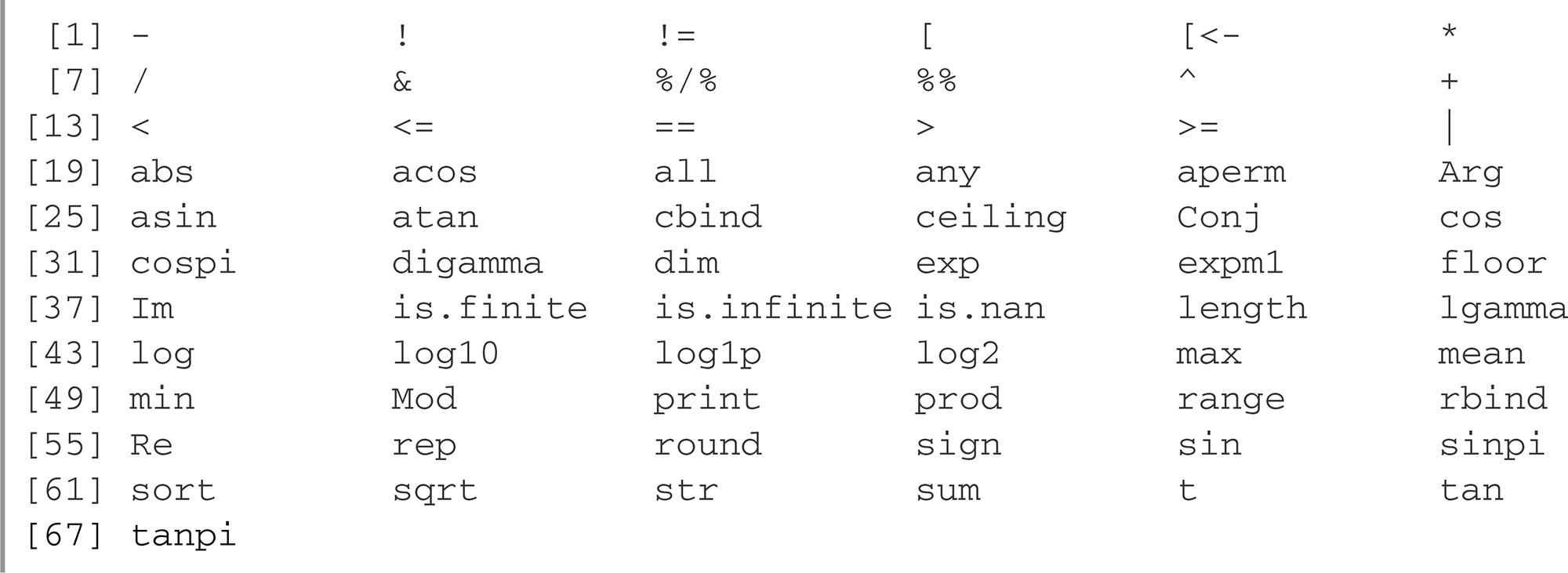
This means that you can often write the same code for TensorFlow tensors as you would for R arrays.

3.7 Tensor attributes

Unlike R arrays, tensors have some attributes you can access with $:

➊ndim returns a scalar integer, the rank of the tensor, equivalent to length(dim(x)).

Length 1 R vectors are automatically converted to rank 0 tensors, whereas R vectors of length > 1 are converted to rank 1 tensors:

tf_tensor$shape returns a tf.TensorShape object. This a class object with support for undefined or unspecified dimensions, and a variety of methods and properties:

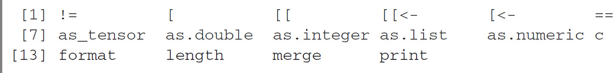
For now, all you need to know is that you can convert a TensorShape to an integer vector with as.integer() (dim(x) is shorthand for as.integer(x$shape)), and you can construct a TensorShape object manually with the shape() function:

tf_tensor$dtype returns the data type of the array. TensorFlow provides support for many more data types than base R. For example, base R has one integer type, whereas TensorFlow provides support for 13! The R integer type corresponds to int32. Different data types make different tradeoffs between how much memory they can consume and the range of values they can represent. For example, a tensor with a int8 dtype takes only one-quarter the space in memory as one with dtype int32, but it can only represent integers between –128 and 127, as opposed to –2147483648 to 2147483647.

We’ll also be dealing with floating-point data throughout the book. In R, the default floating numeric datatype, double, is converted to tf.float64:

For the majority of the book, we’ll be using the smaller float32 as the default floating point datatype, trading some accuracy for a smaller memory footprint and faster computation speed:

3.7.1 Tensor shape and reshaping

as_tensor() can also optionally take a shape argument, which you can use to expand a scalar or reshape a tensor. For example, to make an array of zeros, you could write:

For R vectors that are not scalars (length(x) > 1), you can also reshape the tensor, so long as the overall size of the array stays the same:

Note that the tensor was filled row-wise. This is different from R, which fills arrays column-wise:

This difference between row-major and column-major ordering (also known as C and Fortran ordering, respectively) is one of the things to be on the lookout for when converting between R arrays and tensors. R arrays are always Fortran-ordered, and Tensor-Flow tensors are always C-ordered, and the distinction becomes important anytime you are reshaping an array.

When you are working with tensors, reshaping will use C-style ordering. Anytime you are handling R arrays, you can use array_reshape() if you want to be explicit about the reshaping behavior you want:

Finally, array_reshape() and as_tensor() allow you to leave the size of one of the axes unspecified, and it will be automatically inferred using the size of the array and the size of the remaining axes. You can pass -1 or NA for the axis you want inferred:

3.7.2 Tensor slicing

Subsetting tensors is similar to subsetting R arrays, but not identical. Slicing tensors offers some conveniences that R arrays don’t and vice versa.

Tensors allow you to slice with a missing value supplied to one end of a slice range, which implicitly means “the rest of the tensor in that direction” (R arrays don’t offer this slicing convenience). For example, revisiting the example in chapter 2 where we want to slice out a crop of the MNIST images, we could have provided an NA to the slice instead:

Be aware that the expression 15:NA will produce an R error in other contexts; it works only in the brackets of a tensor slicing operation.

It’s also possible to use negative indices. Note that unlike R arrays, negative indices do not drop elements; instead, they indicate the index position relative to the end of the current axis. (Because this is a change from standard R subsetting behavior, a warning is issued the first time a negative slice index is encountered.) To crop the images to patches of 14 × 14 pixels centered in the middle, you could do this:

You can also use the special all_dims() object anytime you want to implicitly capture remaining dimensions, without supplying the exact number of commas (,) required in the call to [. For example, say you want to take the first 100 images only, you can write

instead of

This comes in handy for writing code that can work with tensors of different ranks, for example, taking matching slices of model inputs and targets along the batch dimension.

3.7.3 Tensor broadcasting

We introduced broadcasting in chapter 2. Broadcasting is performed when we have an operation on two different-sized tensors, and we want the smaller tensor to be broadcast to match the shape of the larger tensor. Broadcasting consists of the following two steps:

1. 1 Axes (called broadcast axes) are added to the smaller tensor to match the ndim of the larger tensor.
2. 2 The smaller tensor is repeated alongside these new axes to match the full shape of the larger tensor.

With broadcasting, you can generally perform element-wise operations that take two input tensors if one tensor has shape (a, b, … n, n + 1, … m) and the other has shape (n, n + 1, … m). The broadcasting will then automatically happen for axes a through n - 1.

The following example applies the element-wise + operation to two tensors of different shapes via broadcasting:

➊ The output z has shape (64, 3, 32, 10) like x.

Anytime you want to be explicit about broadcasting semantics, you can use a tf$newaxis to insert a size 1 dimension in a tensor:

3.7.4 The tf module

Tensors need to be created with some initial value. You can generally stick to as_ tensor() for creating tensors, but the tf module also contains many functions for creating tensors. For instance, you could create all-ones or all-zeros tensors, or tensors of values drawn from a random distribution.

➊ Tensor of random values drawn from a normal distribution with mean 0 and standard deviation 1. Equivalent to array(rnorm(3 * 1, mean = 0, sd = 1), dim = c(1, 3).

➋ Tensor of random values drawn from a uniform distribution between 0 and 1. Equivalent to array(runif(3 * 1, min = 0, max = 1), dim = c(1, 3)).

Note that the tf module exposes the full Python TensorFlow API. One thing to be aware of is that the Python API frequently expects integers, whereas a bare R numeric literal like 2 produces a double instead of an integer. In R, we can specify an integer literal by appending an L, as in 2L.

➊ Providing R doubles here gives an error.

➋ Provide integer literals to avoid the error.

When dealing with the tf module, we will often write literal integers with an L suffix where the Python API requires it.

Another thing to be aware of is that functions in the tf module use a 0-based index counting convention, that is, the first element of a list is element 0. For example, if you want to take the mean along the first axis of a 2D array (in other words, the column means of a matrix), you would do so like this:

The corresponding R functions, however, use a 1-based counting convention:

You can easily access the help for functions in the tf module, right from the RStudio IDE. Press F1 while your cursor is over a function in the tf module to open a webpage with the corresponding documentation at www.tensorflow.org.

3.7.5 Constant tensors and variables

A significant difference between R arrays and TensorFlow tensors is that TensorFlow tensors aren’t modifiable: they’re constant. For instance, in R, you can do the following.

Listing 3.1 R arrays are assignable

Try to do the same thing in TensorFlow, and you will get an error: “EagerTensor object does not support item assignment.”

Listing 3.2 TensorFlow tensors are not assignable

➊ This will fail, because a tensor isn't modifiable.

To train a model, we’ll need to update its state, which is a set of tensors. If tensors aren’t modifiable, how do we do this? That’s where variables come in. tf$Variable is the class meant to manage modifiable state in TensorFlow. You’ve already briefly seen it in action in the training loop implementation at the end of chapter 2.

To create a variable, you need to provide some initial value, such as a random tensor.

Listing 3.3 Creating a TensorFlow variable

The state of a variable can be modified in place via its assign method, as follows.

Listing 3.4 Assigning a value to a TensorFlow variable

It also works for a subset of the coefficients.

Listing 3.5 Assigning a value to a subset of a TensorFlow variable

Similarly, assign_add() and assign_sub() are efficient equivalents of x <- x + value and x <- x - value.

Listing 3.6 Using assign_add()

3.7.6 Tensor operations: Doing math in TensorFlow

TensorFlow offers a large collection of tensor operations to express mathematical formulas. Here are a few examples.

Listing 3.7 A few basic math operations

➊ Take the square.

➋ Take the square root.

➌ Add two tensors (element-wise).

➍ Take the product of two tensors (as discussed in chapter 2).

➎ Multiply two tensors (element-wise).

Note that some of these operations are invoked by their corresponding R generics. For example, calling sqrt(x) will call tf$sqrt(x) if x is a tensor.

Importantly, each of the preceding operations is executed on the fly: at any point, you can print the current result, just like regular R code. We call this eager execution.

3.7.7 A second look at the GradientTape API

So far, TensorFlow seems to look a lot like base R, just with different names for functions and some different tensor capabilities. But here’s something R can’t easily do: retrieve the gradient of any differentiable expression with respect to any of its inputs. Just open a tf$GradientTape() scope using with(), apply some computation to one or several input tensors, and retrieve the gradient of the result with respect to the inputs.

Listing 3.8 Using the GradientTape

This is most commonly used to retrieve the gradients of the loss of a model with respect to its weights: gradients <- tape$gradient(loss, weights). You saw this in action in chapter 2.

So far, you’ve only seen the case where the input tensors in tape$gradient() were TensorFlow variables. It’s actually possible for these inputs to be any arbitrary tensor. However, only trainable variables are tracked by default. With a constant tensor, you’d have to manually mark it as being tracked by calling tape$watch() on it.

Listing 3.9 Using GradientTape with constant tensor inputs

Why is this necessary? Because it would be too expensive to preemptively store the information required to compute the gradient of anything with respect to anything. To avoid wasting resources, the tape needs to know what to watch. Trainable variables are watched by default because computing the gradient of a loss with regard to a list of trainable variables is the most common use of the gradient tape.

The gradient tape is a powerful utility, even capable of computing second-order gradients, that is to say, the gradient of a gradient. For instance, the gradient of the position of an object with regard to time is the speed of that object, and the second-order gradient is its acceleration.

If you measure the position of a falling apple along a vertical axis over time and find that it verifies position(time) = 4.9 * time ^ 2, what is its acceleration? Let’s use two nested gradient tapes to find out.

Listing 3.10 Using nested gradient tapes to compute second-order gradients

➊ We use the outer tape to compute the gradient of the gradient from the inner tape. Naturally, the answer is 4.9 * 2 = 9.8.

3.7.8 An end-to-end example: A linear classifier in pure TensorFlow

You know about tensors, variables, and tensor operations, and you know how to compute gradients. That’s enough to build any machine learning model based on gradient descent. And you’re only at chapter 3!

In a machine learning job interview, you may be asked to implement a linear classifier from scratch in TensorFlow: a very simple task that serves as a filter between candidates who have some minimal machine learning background and those who don’t. Let’s get you past that filter and use your newfound knowledge of TensorFlow to implement such a linear classifier.

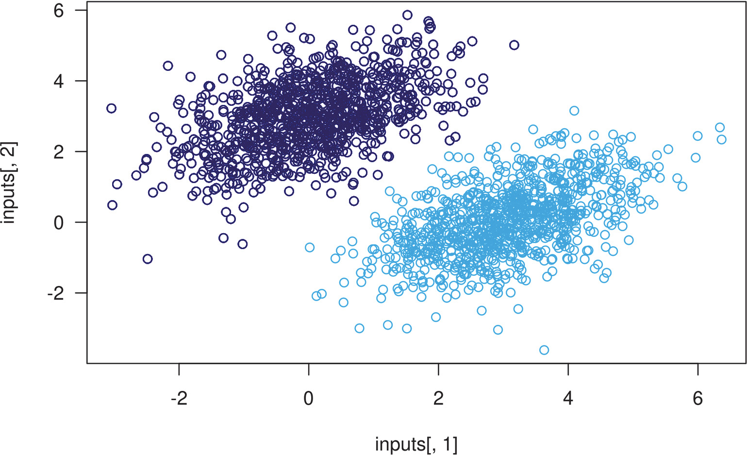
First, let’s come up with some nicely linearly separable synthetic data to work with: two classes of points in a 2D plane. We’ll generate each class of points by drawing their coordinates from a random distribution with a specific covariance matrix and a specific mean. Intuitively, the covariance matrix describes the shape of the point cloud, and the mean describes its position in the plane. We’ll reuse the same covariance matrix for both point clouds, but we’ll use two different mean values—the point clouds will have the same shape, but different positions.

Listing 3.11 Generating two classes of random points in a 2D plane

➊ Generate the first class of points: 1,000 random 2D points. Sigma corresponds to an oval-like point cloud oriented from bottom left to top right.

➋ Generate the other class of points with a different mean and the same covariance matrix.

In the preceding code, negative_samples and positive_samples are both arrays with shape (1000, 2). Let’s stack them into a single array with shape (2000, 2).

Listing 3.12 Stacking the two classes into an array with shape (2000, 2)

Let’s generate the corresponding target labels, an array of zeros and ones of shape (2000, 1), where targets[i, 1] is 0 if inputs[i] belongs to class 1 (and inversely).

Listing 3.13 Generating the corresponding targets (0 and 1)

Next, let’s plot our data.

Listing 3.14 Plotting the two point classes

Now let’s create a linear classifier that can learn to separate these two blobs. A linear classifier is an affine transformation (prediction = W • input + b) trained to minimize the square of the difference between predictions and the targets. As you’ll see, it’s actually a much simpler example than the end-to-end example of a toy two-layer neural network you saw at the end of chapter 2. However, this time you should be able to understand everything about the code, line by line.

Let’s create our variables, W and b, initialized with random values and with zeros, respectively.

Listing 3.15 Creating the linear classifier variables

➊ The inputs will be 2D points.

➋ The output predictions will be a single score per sample (close to 0 if the sample is predicted to be in class 0, and close to 1 if the sample is predicted to be in class 1).

Here’s our forward pass function.

Listing 3.16 The forward pass function

Because our linear classifier operates on 2D inputs, W is really just two scalar coefficients, w1 and w2: W = [[w1], [w2]]. Meanwhile, b is a single scalar coefficient. As such, for a given input point [x, y], its prediction value is prediction = [[w1], [w2]] • [x, y] + b = w1 * x + w2 * y + b.

The following listing shows our loss function.

Listing 3.17 The mean squared error loss function

➊ per_sample_losses will be a tensor with the same shape as targets and predictions, containing per-sample loss scores.

➋ We need to average these per-sample loss scores into a single scalar loss value: this is what mean() does.

Note that in square_loss(), both targets and predictions can be tensors, but they don’t have to be. This is one of the niceties of the R interface—generics like mean(), ^, and - allow you to write the same code for tensors as you would for R arrays. When targets and predictions are tensors, the generics will dispatch to functions in the tf module. We can also write the equivalent square_loss using functions from the tf module directly:

Next is the training step, which receives some training data and updates the weights W and b so as to minimize the loss on the data.

Listing 3.18 The training step function

➊ Forward pass, inside a gradient tape scope

➋ Retrieve the gradient of the loss with regard to weights.

➌ Update the weights.

For simplicity, we’ll do batch training instead of mini-batch training: we’ll run each training step (gradient computation and weight update) for all the data, rather than iterate over the data in small batches. On one hand, this means that each training step will take much longer to run, because we’ll compute the forward pass and the gradients for 2,000 samples at once. On the other hand, each gradient update will be much more effective at reducing the loss on the training data, because it will encompass information from all training samples instead of, say, only 128 random samples. As a result, we will need many fewer steps of training, and we should use a larger learning rate than we would typically use for mini-batch training (we’ll use learning_rate = 0.1, defined in listing 3.18).

Listing 3.19 The batch training loop

After 40 steps, the training loss seems to have stabilized around 0.025. Let’s plot how our linear model classifies the training data points. Because our targets are zeros and ones, a given input point will be classified as 0 if its prediction value is below 0.5, and as 1 if it is above 0.5:

➊ Convert tensors to R arrays for plotting.

Recall that the prediction value for a given point [x, y] is simply prediction == [[w1], [w2]] • [x, y] + b == w1 * x + w2 * y + b. Thus, class 1 is defined as (w1 * x + w2 * y + b) < 0.5, and class 2 is defined as (w1 * x + w2 * y + b) > 0.5. You’ll notice that what you’re looking at is really the equation of a line in the 2D plane: w1 * x + w2 * y + b = 0.5. Above the line is class 1, and below the line is class 0. You may be used to seeing line equations in the format y = a * x + b; in the same format, our line becomes y = - w1 / w2 * x + (0.5 - b) / w2.

Let’s plot this line:

➊ Plot our model's predictions.

➋ These are our line's equation values.

➌ Plot our line.

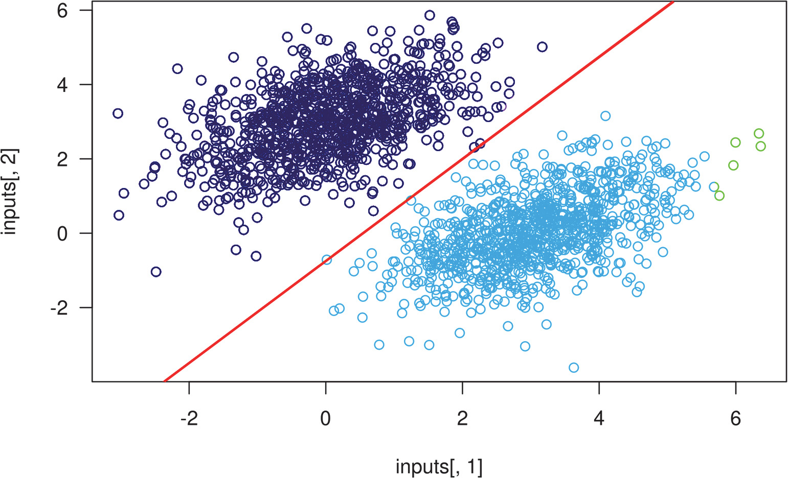
This is really what a linear classifier is all about: finding the parameters of a line (or, in higher-dimensional spaces, a hyperplane) neatly separating two classes of data.

3.8 Anatomy of a neural network: Understanding core Keras APIs

At this point, you know the basics of TensorFlow, and you can use it to implement a toy model from scratch, such as the batch linear classifier in the previous section, or the toy neural network at the end of chapter 2. That’s a solid foundation to build upon. It’s now time to move on to a more productive, more robust path to deep learning: the Keras API.

3.8.1 Layers: The building blocks of deep learning

The fundamental data structure in neural networks is the layer, to which you were introduced in chapter 2. A layer is a data-processing module that takes as input one or more tensors and that outputs one or more tensors. Some layers are stateless, but more frequently layers have a state: the layer’s weights, one or several tensors learned with stochastic gradient descent, which together contain the network’s knowledge.

Different types of layers are appropriate for different tensor formats and different types of data processing. For instance, simple vector data, stored in rank 2 tensors of shape (samples, features), is often processed by densely connected layers, also called fully connected or dense layers (built by the layer_dense() function in Keras). Sequence data, stored in rank 3 tensors of shape (samples, timesteps, features), is typically processed by recurrent layers, such as an LSTM layer (layer_lstm()), or 1D convolution layers (layer_conv_1d()). Image data, stored in rank 4 tensors, is usually processed by 2D convolution layers (layer_conv_2d()).

You can think of layers as the LEGO bricks of deep learning, a metaphor that is made explicit by Keras. Building deep learning models in Keras is done by clipping together compatible layers to form useful data-transformation pipelines.

THE LAYER CLASS IN KERAS

A simple API should have a single abstraction around which everything is centered. In Keras, that’s the Layer class. Everything in Keras is either a Layer or something that closely interacts with a Layer.

A Layer is an object that encapsulates some state (weights) and some computation (a forward pass). The weights are typically defined in a build() method (although they could also be created in the initialize() method), and the computation is defined in the call() method.

In the previous chapter, we implemented a layer_naive_dense() that contained two weights, W and b, and applied the computation output = activation(dot(input, W) + b). This is what the same layer would look like in Keras.

Listing 3.20 Implementing a dense layer as a Keras Layer class

➊ Weight creation takes place in the build() method.

➋ Take the last dim.

➌ add_weight() is a shortcut method for creating weights. It is also possible to create standalone variables and assign them as layer attributes, like this: self$W < - tf$Variable(tf$random$normal(w_shape)).

➍ We define the forward pass computation in the call() method.

This time, instead of building up an empty R environment, we use the new_layer_ class() function provided by Keras. new_layer_class() returns a layer instance generator, just like layer_naive_dense() in chapter 2, but it also provides some additional convenient features for us (like composability with %>%, which we’ll cover in a moment).

In the next section, we’ll cover in detail the purpose of these build() and call() methods. Don’t worry if you don’t understand everything just yet!

Layers can be instantiated simply by calling a Keras function that starts with the layer_ prefix. Then, once instantiated, a layer instance can be used just like a function, taking as input a TensorFlow tensor:

➊ Instantiate our layer, defined previously.

➋ Create some test inputs.

➌ Call the layer on the inputs, just like a function.

You’re probably wondering, why did we have to implement call() and build(), because we ended up using our layer by plainly calling it? It’s because we want to be able to create the state just in time. Let’s see how that works.

AUTOMATIC SHAPE INFERENCE: BUILDING LAYERS ON THE FLY

Just like with LEGO bricks, you can only “clip” together layers that are compatible. The notion of layer compatibility here refers specifically to the fact that every layer will accept only input tensors of a certain shape and will return output tensors of a certain shape. Consider the following example:

➊ A dense layer with 32 output units

This layer will return a tensor where the first dimension has been transformed to be 32. It can only be connected to a downstream layer that expects 32-dimensional vectors as its input.

When using Keras, you don’t have to worry about size compatibility most of the time, because the layers you add to your models are dynamically built to match the shape of the incoming layer. For instance, suppose you write the following:

The layers didn’t receive any information about the shape of their inputs—instead, they automatically inferred their input shape as being the shape of the first inputs they see. In the toy version of the dense layer we implemented in chapter 2 (which we named layer_naive_dense()), we had to pass the layer’s input size explicitly to the constructor to be able to create its weights. That’s not ideal, because it would lead to models that look like the following code snippet, where each new layer needs to be made aware of the shape of the layer before it:

It would be even worse if the rules used by a layer to produce its output shape are complex. For instance, what if our layer returned outputs of shape if (input_size %% 2 == 0) c(batch, input_size * 2) else c(input_size * 3)?

If we were to reimplement layer_naive_dense() as a Keras layer capable of automatic shape inference, it would look like the previous layer_simple_dense() layer (see listing 3.20), with its build() and call() methods.

In layer_simple_dense(), we no longer create weights in the constructor like in the layer_naive_dense() example; instead, we create them in a dedicated state-creation method, build(), which receives as an argument the first input shape seen by the layer. The build() method is called automatically the first time the layer is called. In fact, the function that’s actually called when you call a layer is not call() directly but something that optionally first calls build() before calling call().

The function that’s called when you call a layer schematically looks like this:

With automatic shape inference, our previous example becomes simple and neat:

Note that automatic shape inference is not the only thing that the layer class handles. It takes care of many more things, in particular routing between eager and graph execution (a concept you’ll learn about in chapter 7) and input masking (which we’ll cover in chapter 11). For now, just remember: when implementing your own layers, put the forward pass in the call() method.

3.8.2 From layers to models

A deep learning model is a graph of layers. In Keras, that’s the Model type. Until now, you’ve only seen sequential models, which are simple stacks of layers, mapping a single input to a single output. But as you move forward, you’ll be exposed to a much broader variety of network topologies. These are some common ones:

• Two-branch networks
• Multihead network
• Residual connection

Network topology can get quite involved. For instance, figure 3.2 shows the topology of the graph of layers of a Transformer, a common architecture designed to process text data.

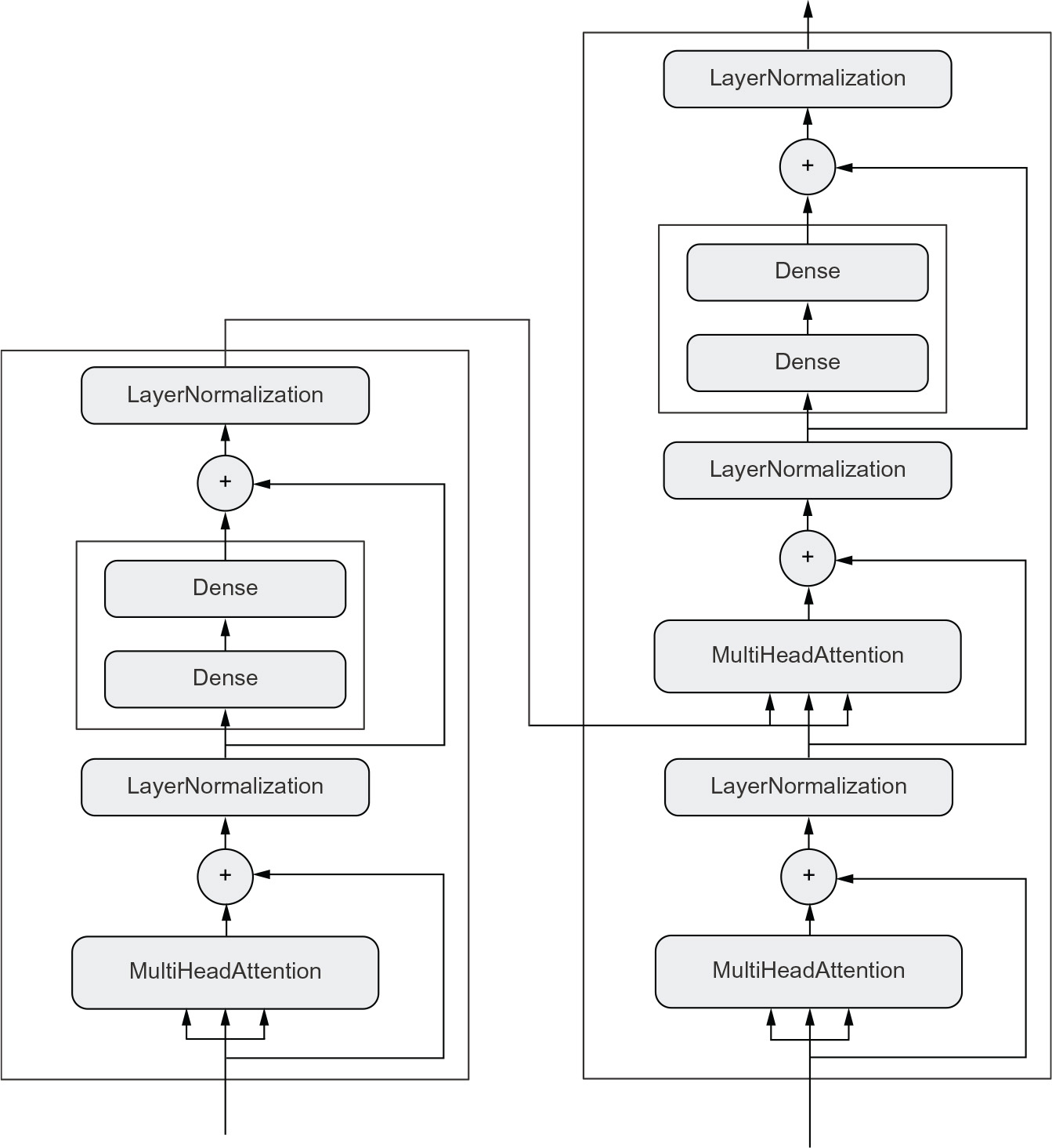
Figure 3.2 The Transformer architecture (covered in chapter 11). There’s a lot going on here. Throughout the next few chapters, you’ll climb your way up to understanding it.

There are generally two ways of building such models in Keras: you could directly define a new_model_class(), or you could use the Functional API, which lets you do more with less code. We’ll cover both approaches in chapter 7.

The topology of a model defines a hypothesis space. You may remember that in chapter 1 we described machine learning as searching for useful representations of some input data, within a predefined space of possibilities, using guidance from a feedback signal. By choosing a network topology, you constrain your space of possibilities (hypothesis space) to a specific series of tensor operations, mapping input data to output data. What you’ll then be searching for is a good set of values for the weight tensors involved in these tensor operations.

To learn from data, you have to make assumptions about it. These assumptions define what can be learned. As such, the structure of your hypothesis space—the architecture of your model—is extremely important. It encodes the assumptions you make about your problem—the prior knowledge that the model starts with. For instance, if you’re working on a two-class classification problem with a model made of a single layer_dense() with no activation (a pure affine transformation), you are assuming that your two classes are linearly separable.

Picking the right network architecture is more an art than a science, and although you can rely on some best practices and principles, only practice can help you become a proper neural network architect. The next few chapters will both teach you explicit principles for building neural networks and help you develop intuition as to what works or doesn’t work for specific problems. You’ll build a solid intuition about what type of model architectures work for different kinds of problems, how to build these networks in practice, how to pick the right learning configuration, and how to tweak a model until it yields the results you want to see.

3.8.3 The “compile” step: Configuring the learning process

Once the model architecture is defined, you still have to choose three more things:

• Loss function (objective function)—The quantity that will be minimized during training. It represents a measure of success for the task at hand.
• Optimizer—Determines how the network will be updated based on the loss function. It implements a specific variant of stochastic gradient descent (SGD).
• Metrics—The measures of success you want to monitor during training and validation, such as classification accuracy. Unlike the loss, training will not optimize directly for these metrics. As such, metrics don’t need to be differentiable.

Once you’ve picked your loss, optimizer, and metrics, you can use the compile() and fit() methods to start training your model. Alternatively, you could also write your own custom training loops—we’ll cover how to do this in chapter 7. It’s a lot more work! For now, let’s take a look at compile() and fit().

The compile() method configures the training process—you’ve already been introduced to it in your very first neural network example in chapter 2. It takes the arguments optimizer, loss, and metrics:

➊ Define a linear classifier.

➋ Specify the optimizer by name: RMSprop (case-insensitive).

➌ Specify the loss by name: mean squared error.

➍ Specify (potentially multiple) metrics: in this case, only accuracy.

In the preceding call to compile(), we passed the optimizer, loss, and metrics as strings (such as “rmsprop”). These strings are actually shortcuts that are converted to R objects. For instance, “rmsprop” becomes optimizer_rmsprop(). Importantly, it’s also possible to specify these arguments as object instances:

This is useful if you want to pass your own custom losses or metrics, or if you want to further configure the objects you’re using—for instance, by passing a learning_rate argument to the optimizer:

In chapter 7, we’ll cover how to create custom losses and metrics. In general, you won’t have to create your own losses, metrics, or optimizers from scratch, because Keras offers a wide range of built-in options that is likely to include what you need.

Optimizers:

Losses:

Metrics:

Throughout this book, you’ll see concrete applications of many of these options.

3.8.4 Picking a loss function

Choosing the right loss function for the right problem is extremely important: your network will take any shortcut it can to minimize the loss, so if the objective doesn’t fully correlate with success for the task at hand, your network will end up doing things you may not have wanted. Imagine a stupid, omnipotent AI trained via SGD with this poorly chosen objective function: “maximizing the average well-being of all humans alive.” To make its job easier, this AI might choose to kill all humans except a few and focus on the well-being of the remaining ones, because average well-being isn’t affected by how many humans are left. That might not be what you intended! Just remember that all neural networks you build will be just as ruthless in lowering their loss function, so choose the objective wisely, or you’ll have to face unintended side effects.

Fortunately, when it comes to common problems such as classification, regression, and sequence prediction, you can follow simple guidelines to choose the correct loss. For instance, you’ll use binary cross-entropy for a two-class classification problem, categorical cross-entropy for a many-class classification problem, and so on. Only when you’re working on truly new research problems will you have to develop your own loss functions. In the next few chapters, we’ll detail explicitly which loss functions to choose for a wide range of common tasks.

3.8.5 Understanding the fit() method

After compile() comes fit(). The fit() method implements the training loop itself. These are its key arguments:

• The data (inputs and targets) to train on. It will typically be passed either in the form of R arrays, tensors, or a TensorFlow Dataset object. You’ll learn more about the tfdatasets API in the next chapters.
• The number of epochs to train for: how many times the training loop should iterate over the data passed.
• The batch size to use within each epoch of mini-batch gradient descent: the number of training examples considered to compute the gradients for one weight update step

Listing 3.21 Calling fit() with R arrays

➊ The input examples, as an R array

➋ The corresponding training targets, as an R array

➌ The training loop will iterate over the data five times.

➍ The training loop will iterate over the data in batches of 128 examples.

The call to fit() returns a history object. This object contains a metrics property, which is a named list of their per-epoch values for “loss” and specific metric names:

3.8.6 Monitoring loss and metrics on validation data

The goal of machine learning is not to obtain models that perform well on the training data, which is easy—all you have to do is follow the gradient. The goal is to obtain models that perform well in general, and particularly on data points that the model has never encountered before. Just because a model performs well on its training data doesn’t mean it will perform well on data it has never seen! For instance, it’s possible that your model could end up merely memorizing a mapping between your training samples and their targets, which would be useless for the task of predicting targets for data the model has never seen before. We’ll go over this point in much more detail in chapter 5.

To keep an eye on how the model does on new data, it’s standard practice to reserve a subset of the training data as validation data: you won’t be training the model on this data, but you will use it to compute a loss value and metrics value. You do this by using the validation_data argument in fit(). Like the training data, the validation data could be passed as R arrays or as a TensorFlow Dataset object.

Listing 3.22 Using the validation_data argument

➊ Reserve 30% of the training inputs and targets for validation (we'll exclude these samples from training and reserve them to compute the validation loss and metrics).

➋ Generate num_validation_samples random integers, in the range of [1, n_cases].

➌ Pass drop = FALSE to prevent the R array [ method from dropping the size-1 dimension, and instead return an array with shape (num_validation_ samples, 1).

➍ Training data, used to update the weights of the model

➎ Validation data, used only to monitor the validation loss and metrics

The value of the loss on the validation data is called the validation loss, to distinguish it from the training loss. Note that it’s essential to keep the training data and validation data strictly separate: the purpose of validation is to monitor whether what the model is learning is actually useful on new data. If any of the validation data has been seen by the model during training, your validation loss and metrics will be flawed.

Note that if you want to compute the validation loss and metrics after the training is complete, you can call the evaluate() method:

evaluate() will iterate in batches (of size batch_size) over the data passed and return numeric vector, where the first entry is the validation loss and the following entries are the validation metrics. If the model has no metrics, only the validation loss is returned (an R vector of length 1).

3.8.7 Inference: Using a model after training

Once you’ve trained your model, you’re going to want to use it to make predictions on new data. This is called inference. To do this, a naive approach would simply be to call the model:

➊ Take an R array or TensorFlow tensor and returns a TensorFlow tensor.

However, this will process all inputs in new_inputs at once, which may not be feasible if you’re looking at a lot of data (in particular, it may require more memory than your GPU has).

A better way to do inference is to use the predict() method. It will iterate over the data in small batches and return an R array of predictions. And unlike calling the model, it can also process TensorFlow Dataset objects:

➊ Take an R array or a TF Dataset and return an R array.

For instance, if we use predict() on some of our validation data with the linear model we trained earlier, we get scalar scores that correspond to the model’s prediction for each input sample:

For now, this is all you need to know about Keras models. You are ready to move on to solving real-world machine learning problems with Keras in the next chapter.

Summary

• TensorFlow is an industry-strength numerical computing framework that can run on CPU, GPU, or TPU. It can automatically compute the gradient of any differentiable expression, it can be distributed to many devices, and it can export programs to various external runtimes—even JavaScript.
• Keras is the standard API for doing deep learning with TensorFlow. It’s what we’ll use throughout this book
• Key TensorFlow objects include tensors, variables, tensor operations, and the gradient tape.
• The central type in Keras is the Layer. A layer encapsulates some weights and some computation. Layers are assembled into models.
• Before you start training a model, you need to pick an optimizer, a loss, and some metrics, which you specify via the model %>% compile() method.
• To train a model, you can use the fit() method, which runs mini-batch gradient descent for you. You can also use it to monitor your loss and metrics on validation data, a set of inputs that the model doesn’t see during training.
• Once your model is trained, you use the model %>% predict() method to generate predictions on new inputs.