1 What is deep learning?

In the past few years, artificial intelligence (AI) has been a subject of intense media hype. Machine learning, deep learning, and AI come up in countless articles, often outside of technology-minded publications. We’re promised a future of intelligent chatbots, self-driving cars, and virtual assistants—a future sometimes painted in a grim light and other times as utopian, where human jobs will be scarce and most economic activity will be handled by robots or AI agents. For a future or current practitioner of machine learning, it’s important to be able to recognize the signal amid the noise, so that you can tell world-changing developments from overhyped press releases. Our future is at stake, and it’s a future in which you have an active role to play: after reading this book, you’ll be one of those who develop those AI systems. So let’s tackle these questions: What has deep learning achieved so far? How significant is it? Where are we headed next? Should you believe the hype?

This chapter provides essential context around artificial intelligence, machine learning, and deep learning.

1.1 Artificial intelligence, machine learning, and deep learning

First, we need to define clearly what we’re talking about when we mention AI. What are artificial intelligence, machine learning, and deep learning (see figure 1.1)? How do they relate to each other?

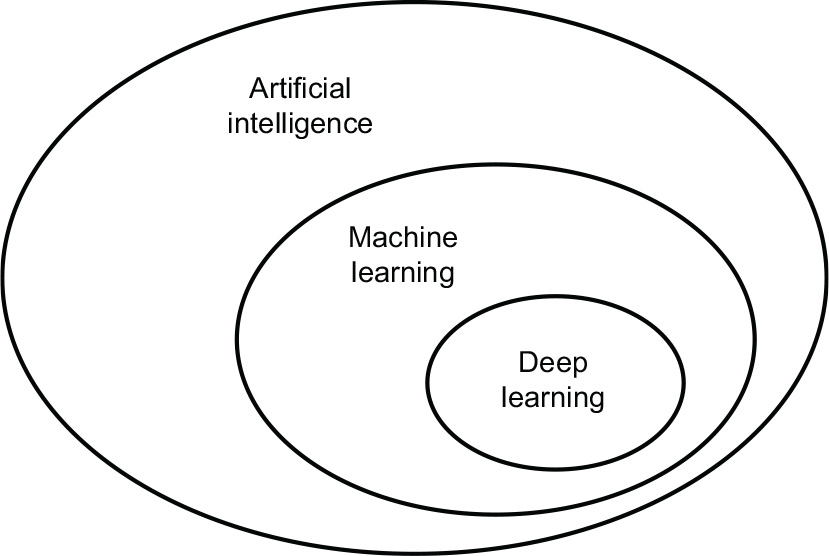
Figure 1.1 Artificial intelligence, machine learning, and deep learning

1.1.1 Artificial intelligence

Artificial intelligence was born in the 1950s, when a handful of pioneers from the nascent field of computer science started asking whether computers could be made to “think”—a question whose ramifications we’re still exploring today.

Although many of the underlying ideas had been brewing in the years and even decades prior, “artificial intelligence” finally crystallized as a field of research in 1956, when John McCarthy, then a young assistant professor of mathematics at Dartmouth College, organized a summer workshop under the following proposal:

The study is to proceed on the basis of the conjecture that every aspect of learning or any other feature of intelligence can in principle be so precisely described that a machine can be made to simulate it. An attempt will be made to find how to make machines use language, form abstractions and concepts, solve kinds of problems now reserved for humans, and improve themselves. We think that a significant advance can be made in one or more of these problems if a carefully selected group of scientists work on it together for a summer.

At the end of the summer, the workshop concluded without having fully solved the riddle it set out to investigate. Nevertheless, it was attended by many people who would move on to become pioneers in the field, and it set in motion an intellectual revolution that is still ongoing to this day.

Concisely, AI can be described as the effort to automate intellectual tasks normally performed by humans. As such, AI is a general field that encompasses machine learning and deep learning, but that also includes many more approaches that may not involve any learning. Consider that until the 1980s, most AI textbooks didn’t mention “learning” at all! Early chess programs, for instance, involved only hardcoded rules crafted by programmers and didn’t qualify as machine learning. In fact, for a fairly long time, most experts believed that human-level artificial intelligence could be achieved by having programmers handcraft a sufficiently large set of explicit rules for manipulating knowledge stored in explicit databases. This approach is known as symbolic AI. It was the dominant paradigm in AI from the 1950s to the late 1980s, and it reached its peak popularity during the expert systems boom of the 1980s.

Although symbolic AI proved suitable to solve well-defined, logical problems, such as playing chess, it turned out to be intractable to figure out explicit rules for solving more complex, fuzzy problems, such as image classification, speech recognition, or natural language translation. A new approach arose to take symbolic AI’s place: machine learning.

1.1.2 Machine learning

In Victorian England, Lady Ada Lovelace was a friend and collaborator of Charles Babbage, the inventor of the Analytical Engine: the first-known general-purpose mechanical computer. Although visionary and far ahead of its time, the Analytical Engine wasn’t meant as a general-purpose computer when it was designed in the 1830s and 1840s, because the concept of general-purpose computation had yet to be invented. It was merely meant as a way to use mechanical operations to automate certain computations from the field of mathematical analysis—hence the name Analytical Engine. As such, it was the intellectual descendant of earlier attempts at encoding mathematical operations in gear form, such as the Pascaline, or Leibniz’s stepped reckoner, a refined version of the Pascaline. Designed by Blaise Pascal in 1642 (at age 19!), the Pascaline was the world’s first mechanical calculator—it could add, subtract, multiply, or even divide digits.

In 1843, Ada Lovelace remarked on the invention of the Analytical Engine:

The Analytical Engine has no pretensions whatever to originate anything. It can do whatever we know how to order it to perform…. Its province is to assist us in making available what we’re already acquainted with.

Even with 179 years of historical perspective, Lady Lovelace’s observation remains arresting. Could a general-purpose computer “originate” anything, or would it always be bound to dully execute processes we humans fully understand? Could it ever be capable of any original thought? Could it learn from experience? Could it show creativity?

Her remark was later quoted by AI pioneer Alan Turing as “Lady Lovelace’s objection” in his landmark 1950 paper “Computing Machinery and Intelligence,”¹ which introduced the Turing test as well as key concepts that would come to shape AI.² Turing was of the opinion—highly provocative at the time—that computers could in principle be made to emulate all aspects of human intelligence.

The usual way to make a computer do useful work is to have a human programmer write down rules—a computer program—to be followed to turn input data into appropriate answers, just like Lady Lovelace writing down step-by-step instructions for the Analytical Engine to perform. Machine learning turns this around: the machine looks at the input data and the corresponding answers, and figures out what the rules should be (see figure 1.2). A machine learning system is trained rather than explicitly programmed. It’s presented with many examples relevant to a task, and it finds statistical structure in these examples that eventually allows the system to come up with rules for automating the task. For instance, if you wished to automate the task of tagging your vacation pictures, you could present a machine learning system with many examples of pictures already tagged by humans, and the system would learn statistical rules for associating specific pictures to specific tags.

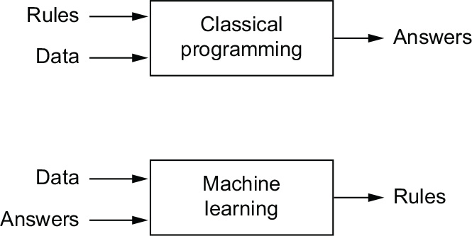
Figure 1.2 Machine learning: A new programming paradigm

Although machine learning started to flourish only in the 1990s, it has quickly become the most popular and most successful subfield of AI, a trend driven by the availability of faster hardware and larger datasets. Machine learning is related to mathematical statistics, but it differs from statistics in several important ways, in the same sense that medicine is related to chemistry but cannot be reduced to chemistry, because medicine deals with its own distinct systems with their own distinct properties. Unlike statistics, machine learning tends to deal with large, complex datasets (such as a dataset of millions of images, each consisting of tens of thousands of pixels) for which classical statistical analysis such as Bayesian analysis would be impractical. As a result, machine learning, and especially deep learning, exhibits comparatively little mathematical theory—maybe too little—and is fundamentally an engineering discipline. Unlike theoretical physics or mathematics, machine learning is a very hands-on field driven by empirical findings and deeply reliant on advances in software and hardware.

1.1.3 Learning rules and representations from data

To define deep learning and understand the difference between deep learning and other machine learning approaches, first we need some idea of what machine learning algorithms do. We just stated that machine learning discovers rules for executing a data processing task, given examples of what’s expected. So, to do machine learning, we need the following three things:

• Input data points—For instance, if the task is speech recognition, these data points could be sound files of people speaking. If the task is image tagging, they could be pictures.
• Examples of the expected output—In a speech-recognition task, these could be human-generated transcripts of sound files. In an image task, expected outputs could be tags such as “dog,” “cat,” and so on.
• A way to measure whether the algorithm is doing a good job—This is necessary to determine the distance between the algorithm’s current output and its expected output. The measurement is used as a feedback signal to adjust the way the algorithm works. This adjustment step is what we call learning.

A machine learning model transforms its input data into meaningful outputs, a process that is “learned” from exposure to known examples of inputs and outputs. Therefore, the central problem in machine learning and deep learning is to meaningfully transform data: in other words, to learn useful representations of the input data at hand— representations that get us closer to the expected output.

Before we go any further: what’s a representation? At its core, it’s a different way to look at data—to represent or encode data. For instance, a color image can be encoded in the RGB format (red-green-blue) or in the HSV format (hue-saturation-value): these are two different representations of the same data. Some tasks that may be difficult with one representation can become easy with another. For example, the task “select all red pixels in the image” is simpler in the RGB format, whereas “make the image less saturated” is simpler in the HSV format. Machine learning models are all about finding appropriate representations for their input data—transformations of the data that make it more amenable to the task at hand.

Let’s make this concrete. Consider an x-axis, a y-axis, and some points represented by their coordinates in the (x, y) system, as shown in figure 1.3.

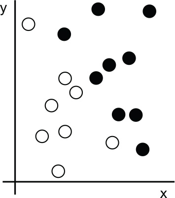
Figure 1.3 Some sample data

As you can see, we have a few white points and a few black points. Let’s say we want to develop an algorithm that can take the coordinates (x, y) of a point and output whether that point is likely to be black or white. In this case, we have the following data:

• The inputs are the coordinates of our points.
• The expected outputs are the colors of our points.
• A way to measure whether our algorithm is doing a good job could be, for instance, the percentage of points that are being correctly classified.

What we need here is a new representation of our data that cleanly separates the white points from the black points. One transformation we could use, among many other possibilities, would be a coordinate change, illustrated in figure 1.4.

In this new coordinate system, the coordinates of our points can be said to be a new representation of our data. And it’s a good one! With this representation, the black/white classification problem can be expressed as a simple rule: “Black points are such that x > 0,” or “White points are such that x < 0.” This new representation, combined with this simple rule, neatly solves the classification problem.

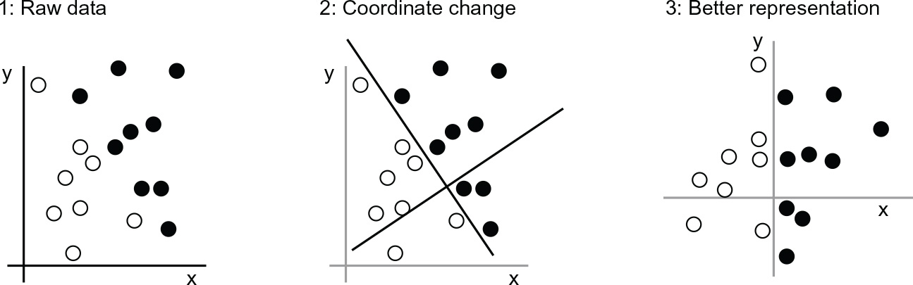
Figure 1.4 Coordinate change

In this case, we defined the coordinate change by hand: we used our human intelligence to come up with our own appropriate representation of the data. This is fine for such an extremely simple problem, but could you do the same if the task was to classify images of handwritten digits? Could you write down explicit, computer-executable image transformations that would illuminate the difference between a 6 and an 8, between a 1 and a 7, across all kinds of different handwriting?

This is possible to an extent. Rules based on representations of digits, such as “number of closed loops” or vertical and horizontal pixel histograms, can do a decent job of telling apart handwritten digits. But finding such useful representations by hand is hard work, and, as you can imagine, the resulting rule-based system is brittle—a nightmare to maintain. Every time you come across a new example of handwriting that breaks your carefully thought-out rules, you will have to add new data transformations and new rules, while taking into account their interaction with every previous rule.

You’re probably thinking, if this process is so painful, could we automate it? What if we tried systematically searching for different sets of automatically generated representations of the data and rules based on them, identifying good ones by using as feedback the percentage of digits being correctly classified in some development data-set? We would then be doing machine learning. Learning, in the context of machine learning, describes an automatic search process for data transformations that produce useful representations of some data, guided by some feedback signal—representations that are amenable to simpler rules solving the task at hand.

These transformations can be coordinate changes (like in our 2-D coordinates classification example), or taking a histogram of pixels and counting loops (like in our digits classification example), but they could also be linear projections, translations, nonlinear operations (such as “select all points such that x > 0”), and so on. Machine learning algorithms aren’t usually creative in finding these transformations; they’re merely searching through a predefined set of operations, called a hypothesis space. For instance, the space of all possible coordinate changes would be our hypothesis space in the 2-D coordinates classification example.

So that’s what machine learning is, concisely: searching for useful representations and rules over some input data, within a predefined space of possibilities, using guidance from a feedback signal. This simple idea allows for solving a remarkably broad range of intellectual tasks, from speech recognition to autonomous driving. Now that you understand what we mean by learning, let’s take a look at what makes deep learning special.

1.1.4 The “deep” in “deep learning”

Deep learning is a specific subfield of machine learning: a new take on learning representations from data that emphasizes learning successive layers of increasingly meaningful representations. The “deep” in “deep learning” isn’t a reference to any kind of deeper understanding achieved by the approach; rather, it stands for this idea of successive layers of representations. How many layers contribute to a model of the data is called the depth of the model. Other appropriate names for the field could have been layered representations learning or hierarchical representations learning. Modern deep learning often involves tens or even hundreds of successive layers of representations, and they’re all learned automatically from exposure to training data. Meanwhile, other approaches to machine learning tend to focus on learning only one or two layers of representations of the data (say, taking a pixel histogram and then applying a classification rule); hence, they’re sometimes called shallow learning.

In deep learning, these layered representations are learned via models called neural networks, structured in literal layers stacked on top of each other. The term “neural network” refers to neurobiology, but although some of the central concepts in deep learning were developed in part by drawing inspiration from our understanding of the brain (in particular, the visual cortex), deep learning models are not models of the brain. There’s no evidence that the brain implements anything like the learning mechanisms used in modern deep learning models. You may come across pop-science articles proclaiming that deep learning works like the brain or was modeled after the brain, but that isn’t the case. It would be confusing and counterproductive for newcomers to the field to think of deep learning as being in any way related to neurobiology; you don’t need that shroud of “just like our minds” mystique and mystery, and you may as well forget anything you may have read about hypothetical links between deep learning and biology. For our purposes, deep learning is a mathematical framework for learning representations from data.

What do the representations learned by a deep learning algorithm look like? Let’s examine how a network several layers deep (see figure 1.5) transforms an image of a digit to recognize what digit it is.

As you can see in figure 1.6, the network transforms the digit image into representations that are increasingly different from the original image and increasingly informative about the final result. You can think of a deep network as a multistage information-distillation process, where information goes through successive filters and comes out increasingly purified (that is, useful with regard to some task).

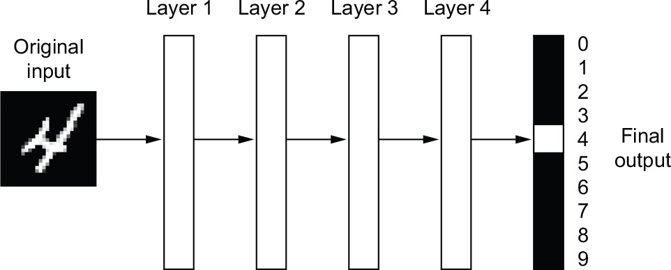
Figure 1.5 A deep neural network for digit classification

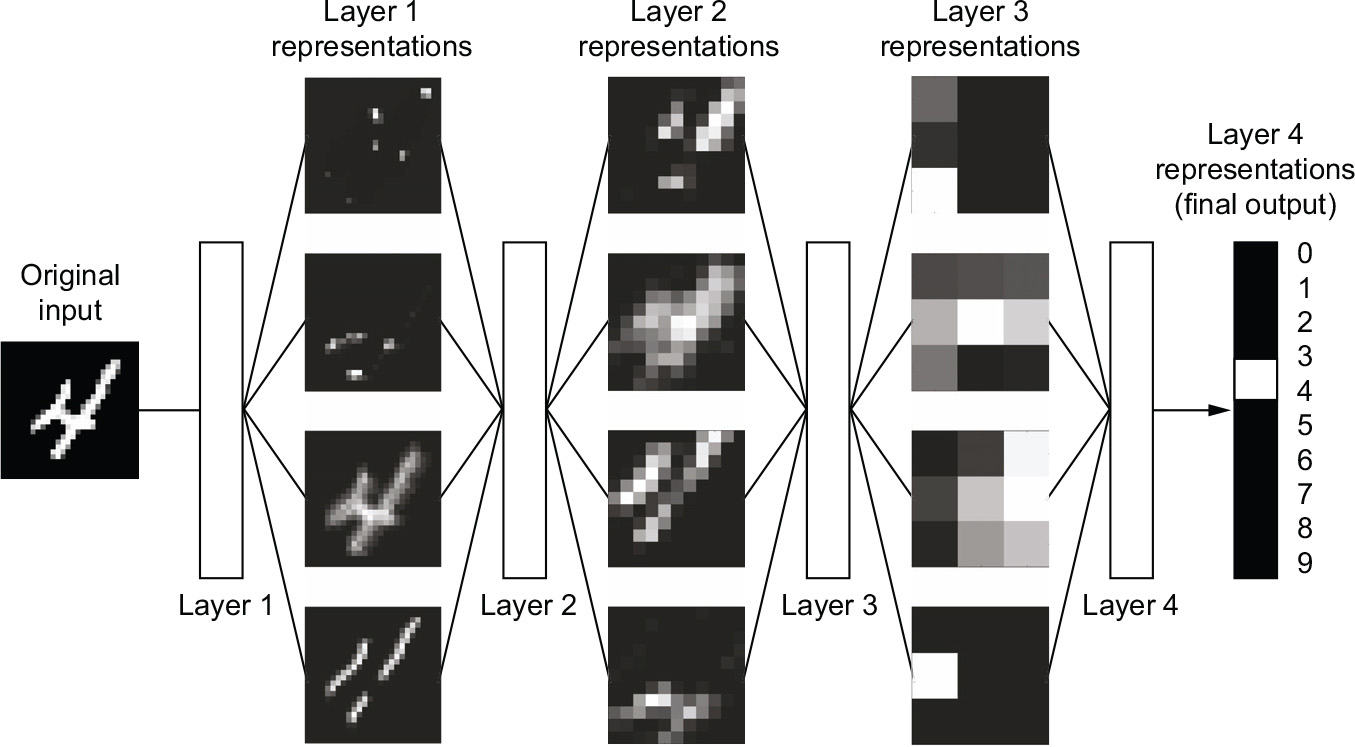
Figure 1.6 Data representations learned by a digit-classification model

So that’s what deep learning is, technically: a multistage way to learn data representations. It’s a simple idea—but, as it turns out, very simple mechanisms, sufficiently scaled, can end up looking like magic.

1.1.5 Understanding how deep learning works, in three figures

At this point, you know that machine learning is about mapping inputs (such as images) to targets (such as the label “cat”), which is done by observing many examples of input and targets. You also know that deep neural networks do this input-to-target mapping via a deep sequence of simple data transformations (layers) and that these data transformations are learned by exposure to examples. Now let’s look at how this learning happens, concretely.

The specification of what a layer does to its input data is stored in the layer’s weights, which in essence are a bunch of numbers. In technical terms, we’d say that the transformation implemented by a layer is parameterized by its weights (see figure 1.7). (Weights are also sometimes called the parameters of a layer.) In this context, learning means finding a set of values for the weights of all layers in a network, such that the network will correctly map example inputs to their associated targets. But here’s the thing: a deep neural network can contain tens of millions of parameters. Finding the correct values for all of them may seem like a daunting task, especially given that modifying the value of one parameter will affect the behavior of all the others!

Figure 1.7 A neural network is parameterized by its weights.

To control something, first you need to be able to observe it. To control the output of a neural network, you need to be able to measure how far this output is from what you expected. This is the job of the loss function of the network, also sometimes called the objective function or cost function. The loss function takes the predictions of the network and the true target (what you wanted the network to output) and computes a distance score, capturing how well the network has done on this specific example (see figure 1.8).

Figure 1.8 A loss function measures the quality of the network’s output.

The fundamental trick in deep learning is to use this score as a feedback signal to adjust the value of the weights a little, in a direction that will lower the loss score for the current example (see figure 1.9). This adjustment is the job of the optimizer, which implements what’s called the backpropagation algorithm: the central algorithm in deep learning. The next chapter explains in more detail how backpropagation works.

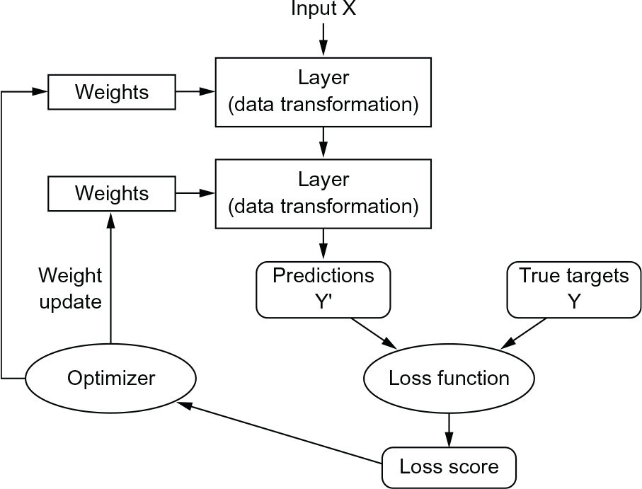
Figure 1.9 The loss score is used as a feedback signal to adjust the weights.

Initially, the weights of the network are assigned random values, so the network merely implements a series of random transformations. Naturally, its output is far from what it should ideally be, and the loss score is accordingly very high. But with every example the network processes, the weights are adjusted a little in the correct direction, and the loss score decreases. This is the training loop, which, repeated a sufficient number of times (typically tens of iterations over thousands of examples), yields weight values that minimize the loss function. A network with a minimal loss is one for which the outputs are as close as they can be to the targets: a trained network. Once again, it’s a simple mechanism that, once scaled, ends up looking like magic.

1.1.6 What deep learning has achieved so far

Although deep learning is a fairly old subfield of machine learning, it rose to prominence only in the early 2010s. In the few years since, it has achieved nothing short of a revolution in the field, producing remarkable results on perceptual tasks and even natural language processing tasks—problems involving skills that seem natural and intuitive to humans but have long been elusive for machines. In particular, deep learning has enabled the following breakthroughs, all in historically difficult areas of machine learning:

• Near-human-level image classification
• Near-human-level speech transcription
• Near-human-level handwriting transcription
• Dramatically improved machine translation
• Dramatically improved text-to-speech conversion
• Digital assistants such as Google Assistant and Amazon Alexa
• Near-human-level autonomous driving
• Improved ad targeting, as used by Google, Baidu, or Bing
• Improved search results on the web
• Ability to answer natural language questions
• Superhuman Go playing

We’re still exploring the full extent of what deep learning can do. We’ve started applying it with great success to a wide variety of problems that were thought to be impossible to solve just a few years ago—automatically transcribing the tens of thousands of ancient manuscripts held in the Vatican’s Apostolic Archive, detecting and classifying plant diseases in fields using a simple smartphone, assisting oncologists or radiologists with interpreting medical imaging data, predicting natural disasters such as floods, hurricanes, or even earthquakes, and so on. With every milestone, we’re getting closer to an age where deep learning assists us in every activity and every field of human endeavor—science, medicine, manufacturing, energy, transportation, software development, agriculture, and even artistic creation.

1.1.7 Don’t believe the short-term hype

Although deep learning has led to remarkable achievements in recent years, expectations for what the field will be able to achieve in the next decade tend to run much higher than what will likely be possible. Although some world-changing applications, like autonomous cars, are already within reach, many more are likely to remain elusive for a long time, such as believable dialogue systems, human-level machine translation across arbitrary languages, and human-level natural language understanding. In particular, talk of human-level general intelligence shouldn’t be taken too seriously. The risk with high expectations for the short term is that, as technology fails to deliver, research investment will dry up, slowing progress for a long time.

This has happened before. Twice in the past, AI went through a cycle of intense optimism followed by disappointment and skepticism, with a dearth of funding as a result. It started with symbolic AI in the 1960s. In those early days, projections about AI were flying high. One of the best-known pioneers and proponents of the symbolic AI approach was Marvin Minsky, who claimed in 1967, “Within a generation… the problem of creating ‘artificial intelligence’ will substantially be solved.” Three years later, in 1970, he made a more precisely quantified prediction: “In from three to eight years we will have a machine with the general intelligence of an average human being.” In 2022, such an achievement still appears to be far in the future—so far that we have no way to predict how long it will take—but in the 1960s and early 1970s, several experts believed it to be right around the corner (as do many people today). A few years later, as these high expectations failed to materialize, researchers and government funds turned away from the field, marking the start of the first AI winter (a reference to a nuclear winter, because this was shortly after the height of the Cold War).

It wouldn’t be the last one. In the 1980s, a new take on symbolic AI, expert systems, started gathering steam among large companies. A few initial success stories triggered a wave of investment, with corporations around the world starting their own in-house AI departments to develop expert systems. Around 1985, companies were spending over $1 billion each year on the technology; but by the early 1990s, these systems had proven expensive to maintain, difficult to scale, and limited in scope, and interest died down. Thus began the second AI winter.

We may be currently witnessing the third cycle of AI hype and disappointment, and we’re still in the phase of intense optimism. It’s best to moderate our expectations for the short term and make sure people less familiar with the technical side of the field have a clear idea of what deep learning can and can’t deliver.

1.1.8 The promise of AI

Although we may have unrealistic short-term expectations for AI, the long-term picture is looking bright. We’re only getting started in applying deep learning to many important problems for which it could prove transformative, from medical diagnoses to digital assistants. AI research has been moving forward amazingly quickly in the past 10 years, in large part due to a level of funding never before seen in the short history of AI, but so far relatively little of this progress has made its way into the products and processes that form our world. Most of the research findings of deep learning aren’t yet applied, or at least are not applied to the full range of problems they could solve across all industries. Your doctor doesn’t yet use AI, and neither does your accountant. You probably don’t use AI technologies very often in your day-to-day life. Of course, you can ask your smartphone simple questions and get reasonable answers, you can get fairly useful product recommendations on Amazon.com, and you can search for “birthday” on Google Photos and instantly find those pictures of your daughter’s birthday party from last month. That’s a far cry from where such technologies used to stand. But such tools are still only accessories to our daily lives. AI has yet to transition to being central to the way we work, think, and live.

Right now, it may seem hard to believe that AI could have a large impact on our world, because it isn’t yet widely deployed—much as, back in 1995, it would have been difficult to believe in the future impact of the internet. Back then, most people didn’t see how the internet was relevant to them and how it was going to change their lives. The same is true for deep learning and AI today. But make no mistake: AI is coming. In a not-so-distant future, AI will be your assistant, even your friend; it will answer your questions, help educate your kids, and watch over your health. It will deliver your groceries to your door and drive you from point A to point B. It will be your interface to an increasingly complex and information-intensive world. And, even more important, AI will help humanity as a whole move forward, by assisting human scientists in new breakthrough discoveries across all scientific fields, from genomics to mathematics.

On the way, we may face a few setbacks and maybe even a new AI winter—in much the same way the internet industry was overhyped in 1998–1999 and suffered from a crash that dried up investment throughout the early 2000s. But we’ll get there eventually. AI will end up being applied to nearly every process that makes up our society and our daily lives, much like the internet is today.

Don’t believe the short-term hype, but do believe in the long-term vision. It may take a while for AI to be deployed to its true potential—a potential the full extent of which no one has yet dared to dream—but AI is coming, and it will transform our world in a fantastic way.

1.2 Before deep learning: A brief history of machine learning

Deep learning has reached a level of public attention and industry investment never before seen in the history of AI, but it isn’t the first successful form of machine learning. It’s safe to say that most of the machine learning algorithms used in the industry today aren’t deep learning algorithms. Deep learning isn’t always the right tool for the job—sometimes there isn’t enough data for deep learning to be applicable, and sometimes the problem is better solved by a different algorithm. If deep learning is your first contact with machine learning, you may find yourself in a situation where all you have is the deep learning hammer, and every machine learning problem starts to look like a nail. The only way not to fall into this trap is to be familiar with other approaches and practice them when appropriate.

A detailed discussion of classical machine learning approaches is outside of the scope of this book, but I’ll briefly go over them and describe the historical context in which they were developed. This will allow us to place deep learning in the broader context of machine learning and better understand where deep learning comes from and why it matters.

1.2.1 Probabilistic modeling

Probabilistic modeling is the application of the principles of statistics to data analysis. It is one of the earliest forms of machine learning, and it’s still widely used to this day. One of the best-known algorithms in this category is the naive Bayes algorithm.

Naive Bayes is a type of machine learning classifier based on applying Bayes’ theorem while assuming that the features in the input data are all independent (a strong, or “naive” assumption, which is where the name comes from). This form of data analysis predates computers and was applied by hand decades before its first computer implementation (most likely dating back to the 1950s). Bayes’ theorem and the foundations of statistics date back to the 18th century, and these are all you need to start using naive Bayes classifiers.

A closely related model is logistic regression (logreg for short), which is sometimes considered to be the “Hello World” of modern machine learning. Don’t be misled by its name—logreg is a classification algorithm rather than a regression algorithm. Much like naive Bayes, logreg predates computing by a long time, yet it’s still useful to this day, thanks to its simple and versatile nature. It’s often the first thing a data scientist will try on a dataset to get a feel for the classification task at hand.

1.2.2 Early neural networks

Early iterations of neural networks have been completely supplanted by the modern variants covered in these pages, but it’s helpful to be aware of how deep learning originated. Although the core ideas of neural networks were investigated in toy forms as early as the 1950s, the approach took decades to get started. For a long time, the missing piece was an efficient way to train large neural networks. This changed in the mid-1980s, when multiple people independently rediscovered the backpropagation algorithm—a way to train chains of parametric operations using gradient-descent optimization (we’ll precisely define these concepts later in the book)—and started applying it to neural networks.

The first successful practical application of neural networks came in 1989 from Bell Labs, when Yann LeCun combined the earlier ideas of convolutional neural networks and backpropagation and applied them to the problem of classifying handwritten digits. The resulting network, dubbed LeNet, was used by the United States Postal Service in the 1990s to automate the reading of ZIP codes on mail envelopes.

1.2.3 Kernel methods

As neural networks started to gain some respect among researchers in the 1990s, thanks to this first success, a new approach to machine learning rose to fame and quickly sent neural networks back to oblivion: kernel methods. Kernel methods are a group of classification algorithms, the best known of which is the Support Vector Machine (SVM). The modern formulation of an SVM was developed by Vladimir Vapnik and Corinna Cortes in the early 1990s at Bell Labs and published in 1995,³ although an older linear formulation was published by Vapnik and Alexey Chervonenkis as early as 1963.⁴

SVM is a classification algorithm that works by finding “decision boundaries” separating two classes (see figure 1.10). SVMs proceed to find these boundaries in the following two steps:

1. 1 The data is mapped to a new high-dimensional representation where the decision boundary can be expressed as a hyperplane (if the data was two-dimensional, as in figure 1.10, a hyperplane would be a straight line).
2. 2 A good decision boundary (a separation hyperplane) is computed by trying to maximize the distance between the hyper-plane and the closest data points from each class, a step called maximizing the margin. This allows the boundary to generalize well to new samples outside of the training dataset.

Figure 1.10 A decision boundary

The technique of mapping data to a high-dimensional representation where a classification problem becomes simpler may look good on paper, but in practice, it’s often computationally intractable. That’s where the kernel trick comes in (the key idea that kernel methods are named after). Here’s the gist of it: to find good decision hyperplanes in the new representation space, you don’t have to explicitly compute the coordinates of your points in the new space; you just need to compute the distance between pairs of points in that space, which can be done efficiently using a kernel function. A kernel function is a computationally tractable operation that maps any two points in your initial space to the distance between these points in your target representation space, completely bypassing the explicit computation of the new representation. Kernel functions are typically crafted by hand rather than learned from data—in the case of an SVM, only the separation hyperplane is learned.

At the time they were developed, SVMs exhibited state-of-the-art performance on simple classification problems and were one of the few machine learning methods backed by extensive theory and amenable to serious mathematical analysis, making them well understood and easily interpretable. Because of these useful properties, SVMs became extremely popular in the field for a long time.

But SVMs proved hard to scale to large datasets and didn’t provide good results for perceptual problems such as image classification. Because an SVM is a shallow method, applying an SVM to perceptual problems requires first extracting useful representations manually (a step called feature engineering), which is difficult and brittle. For instance, if you want to use an SVM to classify handwritten digits, you can’t start from the raw pixels; you should first find by hand useful representations that make the problem more tractable, like the pixel histograms mentioned earlier.

1.2.4 Decision trees, random forests, and gradient-boosting machines

Decision trees are flowchart-like structures that let you classify input data points or predict output values given inputs (see figure 1.11). They’re easy to visualize and interpret. Decision trees learned from data began to receive significant research interest in the 2000s, and by 2010, they were often preferred to kernel methods.

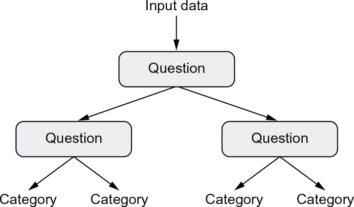
Figure 1.11 A decision tree: The parameters that are learned are the questions about the data. A question could be, for instance, “Is coefficient 2 in the data greater than 3.5?”

In particular, the random forest algorithm introduced a robust, practical take on decision tree learning that involves building a large number of specialized decision trees and then ensembling their outputs. Random forests are applicable to a wide range of problems—you could say that they’re almost always the second-best algorithm for any shallow machine learning task. When the popular machine learning competition website Kaggle (http://kaggle.com) got started in 2010, random forests quickly became a favorite on the platform—until 2014, when gradient-boosting machines took over. A gradient-boosting machine, much like a random forest, is a machine learning technique based on ensembling weak prediction models, generally decision trees. It uses gradient boosting, a way to improve any machine learning model by iteratively training new models that specialize in addressing the weak points of the previous models. Applied to decision trees, the use of the gradient-boosting technique results in models that strictly outperform random forests most of the time, while having similar properties. It may be one of the best, if not the best, algorithm for dealing with nonperceptual data today. Alongside deep learning, it’s one of the most commonly used techniques in Kaggle competitions.

1.2.5 Back to neural networks

Around 2010, although neural networks were almost completely shunned by the scientific community at large, a number of people still working on neural networks started to make important breakthroughs: the groups of Geoffrey Hinton at the University of Toronto, Yoshua Bengio at the University of Montreal, Yann LeCun at New York University, and IDSIA in Switzerland.

In 2011, Dan Cireşan from IDSIA began to win academic image-classification competitions with GPU-trained deep neural networks—the first practical success of modern deep learning. But the watershed moment came in 2012, with the entry of Hinton’s group in the yearly large-scale image-classification challenge, ImageNet (ImageNet Large Scale Visual Recognition Challenge, or ILSVRC for short). The ImageNet challenge was notoriously difficult at the time, consisting of classifying high-resolution color images into 1,000 different categories after training on 1.4 million images. In 2011, the top-five accuracy of the winning model, based on classical approaches to computer vision, was only 74.3%.⁵ Then, in 2012, a team led by Alex Krizhevsky and advised by Geoffrey Hinton was able to achieve a top-five accuracy of 83.6%—a significant breakthrough. The competition has been dominated by deep convolutional neural networks every year since. By 2015, the winner reached an accuracy of 96.4%, and the classification task on ImageNet was considered to be a completely solved problem.

Since 2012, deep convolutional neural networks (convnets) have become the go-to algorithm for all computer vision tasks; more generally, they work on all perceptual tasks. At any major computer vision conference after 2015, it was nearly impossible to find presentations that didn’t involve convnets in some form. At the same time, deep learning has also found applications in many other types of problems, such as natural language processing. It has completely replaced SVMs and decision trees in a wide range of applications. For instance, for several years, the European Organization for Nuclear Research, CERN, used decision tree–based methods for analyzing particle data from the ATLAS detector at the Large Hadron Collider (LHC), but CERN eventually switched to Keras-based deep neural networks due to their higher performance and ease of training on large datasets.

1.2.6 What makes deep learning different?

The primary reason deep learning took off so quickly is that it offered better performance for many problems. But that’s not the only reason. Deep learning also makes problem-solving much easier, because it completely automates what used to be the most crucial step in a machine learning workflow: feature engineering.

Previous machine learning techniques—shallow learning—involved transforming the input data into only one or two successive representation spaces, usually via simple transformations such as high-dimensional nonlinear projections (SVMs) or decision trees. But the refined representations required by complex problems generally can’t be attained by such techniques. As such, humans had to go to great lengths to make the initial input data more amenable to processing by these methods: they had to manually engineer good layers of representations for their data. This is called feature engineering. Deep learning, on the other hand, completely automates this step: with deep learning, you learn all features in one pass rather than having to engineer them yourself. This has greatly simplified machine learning workflows, often replacing sophisticated multistage pipelines with a single, simple, end-to-end deep learning model.

You may ask, if the crux of the issue is to have multiple successive layers of representations, could shallow methods be applied repeatedly to emulate the effects of deep learning? In practice, successive applications of shallow-learning methods produce fast-diminishing returns, because the optimal first representation layer in a three-layer model isn’t the optimal first layer in a one-layer or two-layer model. What is transformative about deep learning is that it allows a model to learn all layers of representation jointly, at the same time, rather than in succession (greedily, as it’s called). With joint feature learning, whenever the model adjusts one of its internal features, all other features that depend on it automatically adapt to the change, without requiring human intervention. Everything is supervised by a single feedback signal: every change in the model serves the end goal. This is much more powerful than greedily stacking shallow models, because it allows for complex, abstract representations to be learned by breaking them down into long series of intermediate spaces (layers); each space is only a simple transformation away from the previous one.

These are the two essential characteristics of how deep learning learns from data: the incremental, layer-by-layer way in which increasingly complex representations are developed, and the fact that these intermediate incremental representations are learned jointly, each layer being updated to follow both the representational needs of the layer above and the needs of the layer below. Together, these two properties have made deep learning vastly more successful than previous approaches to machine learning.

1.2.7 The modern machine learning landscape

A great way to get a sense of the current landscape of machine learning algorithms and tools is to look at machine learning competitions on Kaggle. Due to its highly competitive environment (some contests have thousands of entrants and million-dollar prizes) and to the wide variety of machine learning problems covered, Kaggle offers a realistic way to assess what works and what doesn’t. So, what kind of algorithm is reliably winning competitions? What tools do top entrants use?

In early 2019, Kaggle ran a survey asking teams that ended in the top five of any competition since 2017 which primary software tool they had used in the competition (see figure 1.12). It turns out that top teams tend to use either deep learning methods (most often via the Keras library) or gradient-boosted trees (most often via the LightGBM or XGBoost libraries).

Figure 1.12 Machine learning tools used by top teams on Kaggle

It’s not just competition champions, either. Kaggle also runs a yearly survey among machine learning and data science professionals worldwide. With tens of thousands of respondents, this survey is one of the most reliable sources about the state of the industry. Figure 1.13 shows the percentage of usage of different machine learning software frameworks.

From 2016 to 2020, the entire machine learning and data science industry has been dominated by these two approaches: deep learning and gradient-boosted trees. Specifically, gradient-boosted trees are used for problems where structured data is available, whereas deep learning is used for perceptual problems such as image classification.

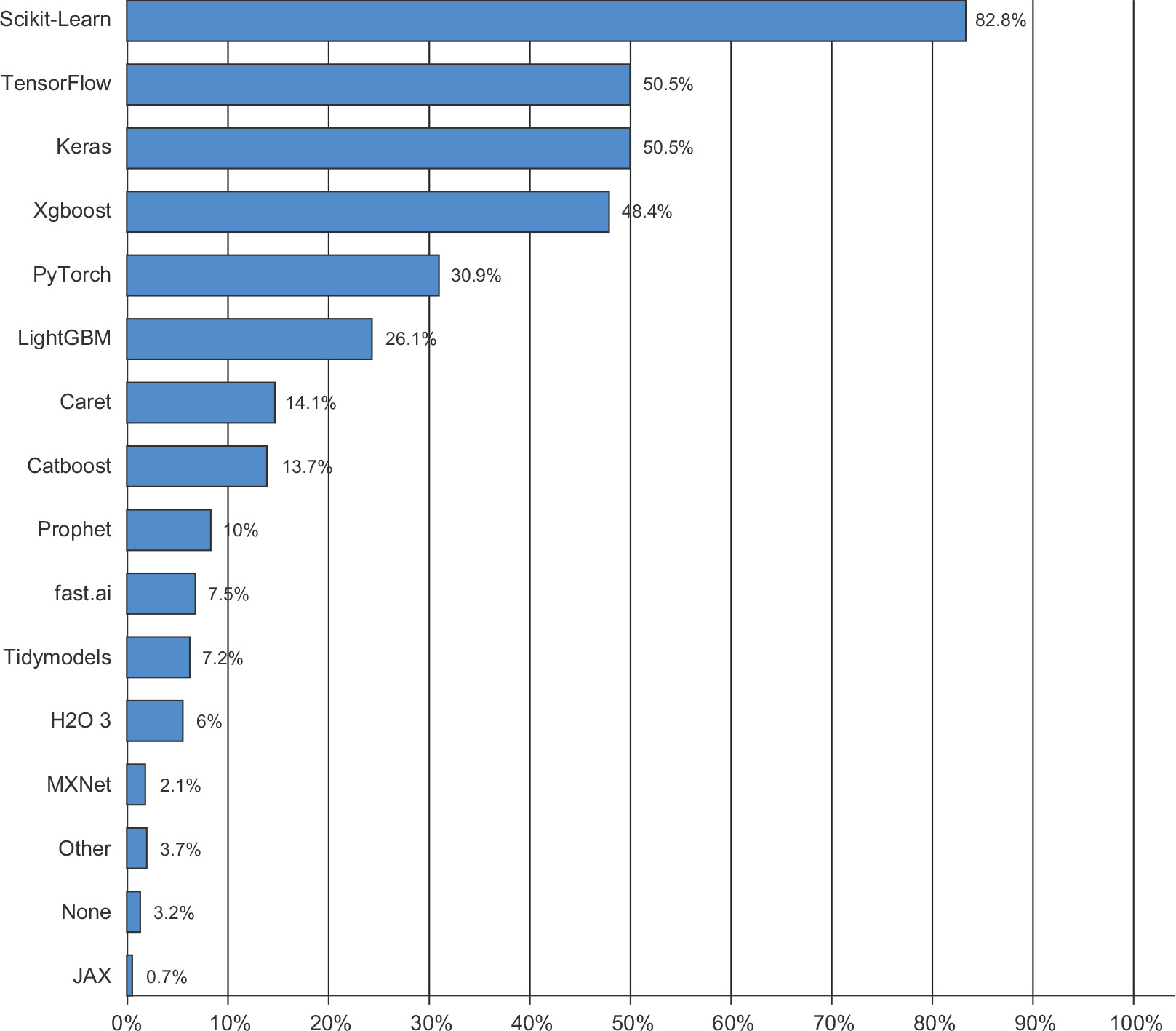
Figure 1.13 Tool usage across the machine learning and data science industry (Source: http://www.kaggle.com/kaggle-survey-2020)

Users of gradient-boosted trees tend to use Scikit-Learn, XGBoost, or LightGBM. Meanwhile, most practitioners of deep learning use Keras, often in combination with its parent framework, TensorFlow. The common point of these tools is they’re all available as R or Python libraries: R and Python are by far the most widely used language for machine learning and data science.

You should be the most familiar with the following two techniques to be successful in applied machine learning today: gradient-boosted trees, for shallow-learning problems; and deep learning, for perceptual problems. In technical terms, this means you’ll need to be familiar with XGBoost and Keras—the libraries that currently dominate Kaggle competitions. With this book in hand, you’re already one big step closer.

1.3 Why deep learning? Why now?

The two key ideas of deep learning for computer vision—convolutional neural networks and backpropagation—were already well understood by 1990. The long short-term memory (LSTM) algorithm, which is fundamental to deep learning for time series, was developed in 1997 and has barely changed since. Why did deep learning take off only after 2012? What changed in these two decades? In general, the following three technical forces are driving advances in machine learning:

• Hardware
• Datasets and benchmarks
• Algorithmic advances

Because the field is guided by experimental findings rather than by theory, algorithmic advances become possible only when appropriate data and hardware are available to try new ideas (or to scale up old ideas, as is often the case). Machine learning isn’t mathematics or physics, where major advances can be done with a pen and a piece of paper. It’s an engineering science.

The real bottlenecks throughout the 1990s and 2000s were data and hardware. But here’s what happened during that time: the internet took off and high-performance graphics chips were developed for the needs of the gaming market.

1.3.1 Hardware

Between 1990 and 2010, off-the-shelf CPUs became faster by a factor of approximately 5,000. As a result, nowadays it’s possible to run small deep learning models on your laptop, whereas this would have been intractable 25 years ago.

But typical deep learning models used in computer vision or speech recognition require orders of magnitude more computational power than your laptop can deliver. Throughout the 2000s, companies like NVIDIA and AMD invested billions of dollars in developing fast, massively parallel chips (graphical processing units, or GPUs) to power the graphics of increasingly photorealistic video games—cheap, single-purpose supercomputers designed to render complex 3-D scenes on your screen in real time. This investment came to benefit the scientific community when, in 2007, NVIDIA launched CUDA (https://developer.nvidia.com/about-cuda), a programming interface for its line of GPUs. A small number of GPUs started replacing massive clusters of CPUs in various highly parallelizable applications, beginning with physics modeling. Deep neural networks, consisting mostly of many small matrix multiplications, are also highly parallelizable, and around 2011, some researchers began to write CUDA implementations of neural nets—Dan Cireşan⁶ and Alex Krizhevsky⁷ were among the first.

What happened is that the gaming market subsidized supercomputing for the next generation of artificial intelligence applications. Sometimes, big things begin as games. The NVIDIA Titan RTX, a GPU that cost $2,500 at the end of 2019, can deliver a peak of 16 teraflops in single precision (16 trillion float32 operations per second). That’s about 500 times more computing power than the world’s fastest supercomputer from 1990, the Intel Touchstone Delta. On a Titan RTX, it takes only a few hours to train an ImageNet model of the sort that would have won the ILSVRC competition around 2012 or 2013. Meanwhile, large companies train deep learning models on clusters of hundreds of GPUs.

What’s more, the deep learning industry has been moving beyond GPUs and is investing in increasingly specialized, efficient chips for deep learning. In 2016, at its annual I/O convention, Google revealed its Tensor Processing Unit (TPU) project: a new chip design developed from the ground up to run deep neural networks significantly faster and far more energy efficiently than top-of-the-line GPUs. In 2020, the third iteration of the TPU card represents 420 teraflops of computing power. That’s 10,000 times more than the Intel Touchstone Delta from 1990.

These TPU cards are designed to be assembled into large-scale configurations, called “pods.” One pod (1024 TPU cards) peaks at 100 petaflops. For scale, that’s about 10% of the peak computing power of the current largest supercomputer, the IBM Summit at Oak Ridge National Lab, which consists of 27,000 NVIDIA GPUs and peaks at around 1.1 exaflops.

1.3.2 Data

AI is sometimes heralded as the new industrial revolution. If deep learning is the steam engine of this revolution, then data is its coal: the raw material that powers our intelligent machines, without which nothing would be possible. When it comes to data, in addition to the exponential progress in storage hardware over the past 20 years (following Moore’s law), the game changer has been the rise of the internet, making it feasible to collect and distribute very large datasets for machine learning. Today, large companies work with image datasets, video datasets, and natural language datasets that couldn’t have been collected without the internet. User-generated image tags on Flickr, for instance, have been a treasure trove of data for computer vision. So are YouTube videos. And Wikipedia is a key dataset for natural language processing.

If there’s one dataset that has been a catalyst for the rise of deep learning, it’s the ImageNet dataset, consisting of 1.4 million images that have been hand annotated with 1,000 image categories (one category per image). But what makes ImageNet special isn’t just its large size but also the yearly competition associated with it.⁸

As Kaggle has been demonstrating since 2010, public competitions are an excellent way to motivate researchers and engineers to push the envelope. Having common benchmarks that researchers compete to beat has greatly helped the rise of deep learning by highlighting its success against classical machine learning approaches.

1.3.3 Algorithms

In addition to hardware and data, until the late 2000s, we were missing a reliable way to train very deep neural networks. As a result, neural networks were still fairly shallow, using only one or two layers of representations; thus, they weren’t able to shine against more-refined shallow methods such as SVMs and random forests. The key issue was that of gradient propagation through deep stacks of layers. The feedback signal used to train neural networks would fade away as the number of layers increased.

This changed around 2009–2010 with the advent of the following simple but important algorithmic improvements that allowed for better gradient propagation:

• Better activation functions for neural layers
• Better weight-initialization schemes, starting with layer-wise pretraining, which was then quickly abandoned
• Better optimization schemes, such as RMSprop and Adam

Only when these improvements began to allow for training models with 10 or more layers did deep learning start to shine. Finally, in 2014, 2015, and 2016, even more advanced ways to improve gradient propagation were discovered, such as batch normalization, residual connections, and depthwise separable convolutions.

Today, we can train models that are arbitrarily deep from scratch. This has unlocked the use of extremely large models, which hold considerable representational power—that is to say, which encode very rich hypothesis spaces. This extreme scalability is one of the defining characteristics of modern deep learning. Large-scale model architectures, which feature tens of layers and tens of millions of parameters, have brought about critical advances both in computer vision (for instance, architectures such as ResNet, Inception, or Xception) and natural language processing (for instance, large Transformer-based architectures such as BERT, GPT-3, or XLNet).

1.3.4 A new wave of investment

As deep learning became the new state of the art for computer vision in 2012–2013, and eventually for all perceptual tasks, industry leaders took note. What followed was a gradual wave of industry investment far beyond anything previously seen in the history of AI (see figure 1.14).

In 2011, right before deep learning took the spotlight, the total venture capital investment in AI worldwide was less than a billion dollars, which went almost entirely to practical applications of shallow machine learning approaches. In 2015, it had risen to over $5 billion, and in 2017, to a staggering $16 billion. Hundreds of startups launched in these few years, trying to capitalize on the deep learning hype. Meanwhile, large tech companies such as Google, Amazon, and Microsoft have invested in internal research departments in amounts that would most likely dwarf the flow of venture-capital money.

Figure 1.14 OECD estimate of total investments in AI startups (Source: http://mng.bz/zGN6)

Machine learning—in particular, deep learning—has become central to the product strategy of these tech giants. In late 2015, Google CEO Sundar Pichai stated, “Machine learning is a core, transformative way by which we’re rethinking how we’re doing everything. We’re thoughtfully applying it across all our products, be it search, ads, YouTube, or Play. And we’re in early days, but you’ll see us—in a systematic way— apply machine learning in all these areas.”⁹

As a result of this wave of investment, the number of people working on deep learning went from a few hundred to tens of thousands in less than 10 years, and research progress has reached a frenetic pace.

1.3.5 The democratization of deep learning

One of the key factors driving this inflow of new faces in deep learning has been the democratization of the toolsets used in the field. In the early days, doing deep learning required significant C++ and CUDA expertise, which few people possessed.

Nowadays, basic R or Python scripting skills suffice to do advanced deep learning research. This has been driven most notably by the development of the TensorFlow library—a symbolic tensor-manipulation frameworks that supports autodifferentiation, greatly simplifying the implementation of new models—and by the rise of user-friendly libraries such as Keras, which makes deep learning as easy as manipulating LEGO bricks. After its release in early 2015, Keras quickly became the go-to deep learning solution for large numbers of new startups, graduate students, and researchers pivoting into the field.

1.3.6 Will it last?

Is there anything special about deep neural networks that makes them the “right” approach for companies to be investing in and for researchers to flock to? Or is deep learning just a fad that may not last? Will we still be using deep neural networks in 20 years?

Deep learning has several properties that justify its status as an AI revolution, and it’s here to stay. We may not be using neural networks two decades from now, but whatever we use will directly inherit from modern deep learning and its core concepts. These important properties can be broadly sorted into the following three categories:

• Simplicity—Deep learning removes the need for feature engineering, replacing complex, brittle, engineering-heavy pipelines with simple, end-to-end trainable models that are typically built using only five or six different tensor operations.
• Scalability—Deep learning is highly amenable to parallelization on GPUs or TPUs, so it can take full advantage of Moore’s law. In addition, deep learning models are trained by iterating over small batches of data, allowing them to be trained on datasets of arbitrary size. (The only bottleneck is the amount of parallel computational power available, which, thanks to Moore’s law, is a fast-moving barrier.)
• Versatility and reusability—Unlike many prior machine learning approaches, deep learning models can be trained on additional data without restarting from scratch, making them viable for continuous online learning—an important property for very large production models. Furthermore, trained deep learning models are repurposable and thus reusable: for instance, it’s possible to take a deep learning model trained for image classification and drop it into a video-processing pipeline. This allows us to reinvest previous work into increasingly complex and powerful models. This also makes deep learning applicable to fairly small datasets.

Deep learning has been in the spotlight for only a few years, and we may not yet have established the full scope of what it can do. With every passing year, we learn about new use cases and engineering improvements that lift previous limitations. Following a scientific revolution, progress generally follows a sigmoid curve: it starts with a period of fast progress, which gradually stabilizes as researchers hit hard limitations, and then further improvements become incremental.

When I was writing the first edition of this book, in 2016, I predicted that deep learning was still in the first half of that sigmoid, with much more transformative progress to come in the following few years. This has proven true in practice—2017 and 2018 have seen the rise of Transformer-based deep learning models for natural language processing, which have been a revolution in the field, while deep learning also kept delivering steady progress in computer vision and speech recognition. Today, in 2022, deep learning seems to have entered the second half of that sigmoid. We should still expect significant progress in the years to come, but we’re probably out of the initial phase of explosive progress.

Today, I’m extremely excited about the deployment of deep learning technology to every problem it can solve—the list is endless. Deep learning is still a revolution in the making, and it will take many years to realize its full potential.

1. ¹ A.M. Turing, “Computing Machinery and Intelligence,” Mind 59, no. 236 (1950): 433–460.
2. ² Although the Turing test has sometimes been interpreted as a literal test—a goal the field of AI should set out to reach—Turing merely meant it as a conceptual device in a philosophical discussion about the nature of cognition.
3. ³ Vladimir Vapnik and Corinna Cortes, “Support-Vector Networks,” Machine Learning 20, no. 3 (1995): 273–297.
4. ⁴ Vladimir Vapnik and Alexey Chervonenkis, “A Note on One Class of Perceptrons,” Automation and Remote Control 25 (1964).
5. ⁵ “Top-five accuracy” measures how often the model selects the correct answer as part of its top five guesses (out of 1,000 possible answers, in the case of ImageNet).
6. ⁶ See “Flexible, High Performance Convolutional Neural Networks for Image Classification,” Proceedings of the 22nd International Joint Conference on Artificial Intelligence (2011), http://mng.bz/nN0K.
7. ⁷ See “ImageNet Classification with Deep Convolutional Neural Networks,” Advances in Neural Information Processing Systems 25 (2012), http://mng.bz/2286.
8. ⁸ The ImageNet Large Scale Visual Recognition Challenge (ILSVRC), http://www.image-net.org/challenges/LSVRC.
9. ⁹ Sundar Pichai, Alphabet earnings call, Oct. 22, 2015.