18
Autoencoders

This chapter is about a particular kind of learning architecture called an autoencoder. One way to think about a standard autoencoder is that it’s a mechanism for compressing input, so it takes up less disk space and can be communicated more quickly, much as an MP3 encoder compresses music, or a JPG encoder compresses an image. The autoencoder gets its name from the idea that it automatically learns, by virtue of training, how best to encode, or represent, the input data. In practice, we usually use autoencoders for two types of jobs: removing the noise from a dataset, and reducing the dimensionality of a dataset.
We begin this chapter by looking at how to compress data while preserving the information we care about. Armed with this information, we look at a tiny autoencoder. We’ll use it to get our bearings and to discuss key ideas about how these systems work and how their version of representing the data lets us manipulate it in meaningful ways. Then we’ll make a bigger autoencoder and look more closely at its data representation. We’ll see that the encoded data has a surprising amount of natural structure. This enables us to use the second half of the autoencoder as a standalone generator. We can feed the generator random inputs and get back new data that looks like the training data but is, in fact, a wholly new piece of data.
We then expand our network’s usefulness by including convolution layers, which enable us to work directly with images and other 2D data. We will train a convolution-based autoencoder to denoise grainy images, giving us back a clean input. We wrap the chapter up with a look at variational autoencoders, which create a more nicely organized representation of the encoded data. This makes it even easier to use the second part as a generator, since we will have better control over what kind of data it will produce.
Introduction to Encoding
Compressing files is useful throughout computing. Many people listen to their music saved in the MP3 format, which can reduce an audio file by a huge amount while still sounding acceptably close to the original (Wikipedia 2020b). We often view images using the JPG format, which can compress image files down by as much as a factor of 20 while still looking acceptably close to the original image (Wikipedia 2020a). In both cases, the compressed file is only an approximation of the original. The more we compress the file (that is, the less information we save), the easier it is to detect the differences between the original and the compressed version.
We refer to the act of compressing data, or reducing the amount of memory required to store it, as encoding. Encoders are part of everyday computer use. We say that both MP3 and JPG take an input and encode it; then we decode or decompress that version to recover or reconstruct some version of the original. Generally speaking, the smaller the compressed file, the less well the recovered version matches the original
The MP3 and JPG encoders are entirely different, but they are both examples of lossy encoding. Let’s see what this means.
Lossless and Lossy Encoding
In previous chapters we used the word loss as a synonym for error, so our network’s error function was also called its loss function. In this section, we use the word with a slightly different meaning, referring to the degradation of a piece of data that has been compressed and then decompressed. The greater the mismatch between the original and the decompressed version, the greater the loss.
The idea of loss, or degradation of the input, is distinct from the idea of making the input smaller. For example, in Chapter 6, we saw how to use Morse code to carry information. The translation of letters to Morse code symbols carries no loss, because we can exactly reconstruct the original message from the Morse version. We say that converting, or encoding, our message into Morse code is a lossless transformation. We’re just changing format, like changing a book’s typeface or type color.
To see where loss can get involved, let’s suppose that we’re camping in the mountains. On a nearby mountain, our friend Sara is enjoying her birthday. We don’t have radios or phones, but both groups have mirrors, and we’ve found we can communicate between the mountains by reflecting sunlight off our mirrors, sending Morse code back and forth. Suppose that we want to send the message, “HAPPY BIRTHDAY SARA BEST WISHES FROM DIANA” (for simplicity, we leave out punctuation). Counting spaces, that’s 42 characters. That’s a lot of mirror-wiggling. We decide to leave out the vowels, and send “HPP BRTHD SR BST WSHS FRM DN” instead. That’s only 28 letters, so we can send this in about two-thirds the time of the full message.
Our new message has lost some information (the vowels) by being compressed in this way. We say that this is a lossy method of compression.
We can’t make a blanket statement about whether it is or isn’t okay to lose some information from any message. If there is loss, then the amount of loss we can tolerate depends on the message and all the context around it. For example, suppose that our friend Sara is camping with her friend Suri, and it just happens that they share a birthday. In this context, “HPP BRTHD SR” is ambiguous, because they can’t tell who we’re addressing.
An easy way to test if a transformation is lossy or lossless is to consider if it can be inverted, or run backward, to recover the original data. In the case of standard Morse code, we can turn our letters into dot-dash patterns and then back to letters again with nothing lost in the process. But when we deleted the vowels from our message, those letters were lost forever. We can usually guess at them, but we’re only guessing and we can get it wrong. Removing the vowels creates a compressed version that is not invertible.
Both MP3 and JPG are lossy systems for compressing data. In fact, they’re very lossy. But both of these compression standards were carefully designed to throw away just the “right” information so that in most everyday cases, we can’t tell the compressed version from the original.
This was achieved by carefully studying the properties of each kind of data and how it was perceived. For example, the MP3 standard is based not just on the properties of sound in general, but on the properties of music and of the human auditory system. In the same way, the JPG algorithm is not only specialized toward the structure of data within images, but it also builds on science describing the human visual system.
In a perfect but impossible world, compressed files are tiny, and their decompressed versions match their corresponding originals perfectly. In the real world, we trade off the fidelity, or accuracy, of the decompressed image for the file size. Generally speaking, the bigger the file, the better the decompressed file matches the original. This makes sense in terms of information theory: a smaller file holds less information than a larger one. When the original file has redundancy, we can exploit that to make a lossless compression in a smaller file (for example, when we compress a text file using the ZIP format). But in general, compression usually implies some loss.
The designers of lossy compression algorithms work hard to selectively lose just the information that matters to us the least for that particular type of file. Often this question of “what matters” to a person is an issue of debate, leading to a variety of different lossy encoders (such as FLAC and AAC for audio, and JPEG and JPEG 2000 for images).
Blending Representations
Later in this chapter, we will find numerical representations of multiple inputs and then blend those to create new data that has aspects of each input. There are two general approaches to blending data. We can describe the first as content blending. That’s where we blend the content of two pieces of data with each other. For example, content blending the images of a cow and zebra gives us something like Figure 18-1.
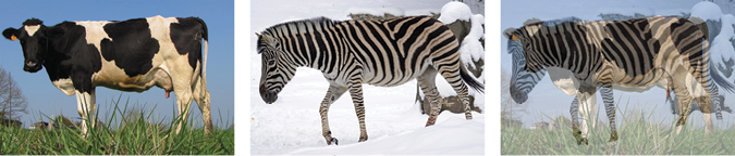
Figure 18-1: Content blending images of a cow and zebra. Scaling each by 50 percent and adding the results together gives us a superposition of the two images, rather than a single animal that’s half cow and half zebra.
The result is a combination of the two images, not an in-between animal that is half cow and half zebra. To get a hybrid animal, we would use a second approach, called parametric blending, or representation blending. Here we work with parameters that describe the thing we’re interested in. By blending two sets of parameters, depending on the nature of the parameters and the algorithm we use to create the object, we can create results that blend the inherent qualities of the things themselves.
For example, suppose we have two circles, each described by a center, radius, and color, as in Figure 18-2.
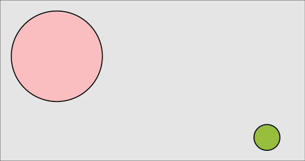
Figure 18-2: Two circles we’d like to blend
If we blend the parameters (that is, we blend the two values representing the x component of the circle’s center with each other, and the two values for y, and similarly for radius and color) then we get an in-between circle, as in Figure 18-3.
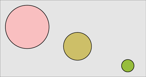
Figure 18-3: Parametric blending of the two circles means blending their parameters (center, radius, and color).
This works well for uncompressed objects. But if we try this with compressed objects, we rarely get reasonable in-between results. The problem is that the compressed form may have little in common with the internal structure that we need to meaningfully blend the objects. For example, let’s take the sounds of the words cherry and orange. These sounds are our objects. We can blend these sounds together by having two people say the words at the same time, creating the audio version of our cow and zebra in Figure 18-1.
We can think of turning these sounds into written language as a form of compression. If it takes a half-second to say the word cherry, then if we use MP3 at a popular compression setting of 128 Kbps, we need about 8,000 bytes (AudioMountain 2020). If we use the Unicode UTF-32 standard (which requires 4 bytes per letter), the written form requires only 24 bytes, which is vastly smaller than 8,000. Since the letters are drawn from the alphabet, which has a given order, we can blend the representations by blending the letters through the alphabet. This isn’t going to work for letters, but let’s follow the process through because a version of this will work for us later.
The first letters of “cherry” and “orange” are C and O. In the alphabet, the region spanned by these letters is CDEFGHIJKLMNO. Right in the middle is the letter I, so that’s the first letter of our blend. When the first letter appears later in the alphabet than the second, as in E to A, we count backward. When there’s an even number of letters in the span, we chosen the earlier one. As shown in Figure 18-4 this blending gives us the sequence IMCPMO.

Figure 18-4: Blending the written words cherry and orange by finding the midpoint of each letter in the alphabet
What we wanted was something that, when uncompressed, sounded like a blend between the sound of cherry and the sound of orange. Saying the word imcpmo out loud definitely does not satisfy that goal. Beyond that, it’s a meaningless string of letters that doesn’t correspond to any fruit, or even any word in English.
In this case, blending the compressed representations doesn’t give us anything like the blended objects. We will see that a remarkable feature of autoencoders, including the variational autoencoder we see at the end of the chapter, is that they do allow us to blend the compressed versions, and (to a point) recover blended versions of the original data.
The Simplest Autoencoder
We can build a deep learning system to figure out a compression scheme for any data we want. The key idea is to create a place in the network where the entire dataset has to be represented by fewer numbers than there are in the input. That, after all, is what compression is all about.
For instance, let’s suppose that our input consists of grayscale images of animals, saved at a resolution of 100 by 100. Each image has 100 × 100 = 10,000 pixels, so our input layer has 10,000 numbers. Let’s arbitrarily say we want to find the best way to represent those images using only 20 numbers.
One way to do this is to build a network as in Figure 18-5. It’s just one layer!

Figure 18-5: Our first encoder is a single dense, or fully connected, layer that turns 10,000 numbers into 20 numbers.
Our input is 10,000 elements, going into a fully connected layer of only 20 neurons. The output of those neurons for any given input is our compressed version of that image. In other words, with just one layer, we’ve built an encoder.
The real trick now would be to be able to recover the original 10,000 pixel values, or even anything close to them, starting from just these 20 numbers. To do that, we follow the encoder with a decoder, as in Figure 18-6. In this case, we just make a fully connected layer with 10,000 neurons, one for each output pixel.
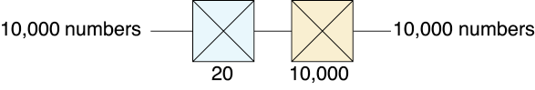
Figure 18-6: An encoder (in blue) turns our 10,000 inputs into 20 variables, then a decoder (in beige) turns those back into 10,000 values.
Because the amount of data is 10,000 elements at the start, 20 in the middle, and 10,000 again at the end, we say that we’ve created a bottleneck. Figure 18-7 shows the idea.

Figure 18-7: We say the middle of a network like the one shown in Figure 18-6 is a bottleneck because it’s shaped like a bottle with a narrow top, or neck.
Now we can train our system. Each input image is also the output target. This tiny autoencoder tries to find the best way to crunch the input into just 20 numbers that can be uncrunched to match the target, which is the input itself. The compressed representation at the bottleneck is called the code, or the latent variables (latent suggests that these values are inherent in the input data, just waiting for us to discover them). Usually we make the bottleneck using a small layer in the middle of a deep network, as in Figure 18-6. Naturally enough, this layer is often called the latent layer or the bottleneck layer. The outputs of the neurons on this layer are the latent variables. The idea is that these values represent the image in some way.
This network has no category labels (as with a categorizer) or targets (as with a regression model). We don’t have any other information for the system other than the input we want it to compress and then decompress. We say that an autoencoder is an example of semi-supervised learning. It sort-of is supervised learning because we give the system explicit goal data (the output should be the same as the input), and it sort-of isn’t supervised learning because we don’t have any manually determined labels or targets on the inputs.
Let’s train our tiny autoencoder of Figure 18-6 on an image of a tiger and see how it does. We’ll feed it the tiger image over and over, encouraging the system to output a full-size image of the tiger, despite the compression down to just 20 numbers at the bottleneck. The loss function compares the pixels of the original tiger with the pixels from the autoencoder’s output and adds up the differences, so the more the pixels differ, the larger the loss. We trained it until it stopped improving. Figure 18-8 shows the result. Each error value shown on the far right is the original pixel value minus the corresponding output pixel value (the pixels were scaled to the range [0,1]).
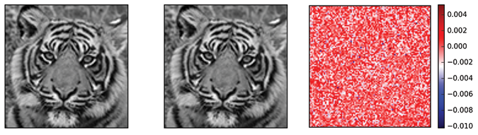
Figure 18-8: Training our autoencoder of Figure 18-6 on a tiger. Left: The original, input tiger. Middle: The output. Right: The pixel-by-pixel differences between the original and output tiger (pixels are in the range [0,1]). The autoencoder seems to have done an amazing job since the bottleneck had only 20 numbers.
This is fantastic! Our system took a picture composed of 10,000 pixel values and crunched them down to 20 numbers, and now it appears to have recovered the entire picture again, right down to the thin, wispy whiskers. The biggest error in any pixel was about 1 part in 100. It looks like we’ve found a fantastic way to do compression!
But wait a second. This doesn’t make sense. There’s just no way to rebuild that tiger image from 20 numbers without doing something sneaky. In this case, the sneaky thing is that the network has utterly overfit and memorized the image. It simply set up all 10,000 output neurons to take those 20 input numbers and reconstruct the original 10,000 input values. Put more bluntly, the network merely memorized the tiger. We didn’t really compress anything at all. Each of the 10,000 inputs went to each of the 20 neurons in the bottleneck layer, requiring 20 × 10,000 = 200,000 weights, and then the 20 bottleneck results all went to each of the 10,000 neurons in the output layer, requiring another 200,000 weights, which then produced the picture of the tiger. We basically found a way to store 10,000 numbers using only 400,000 numbers. Hooray?
In fact, most of those numbers are irrelevant. Remember that each neuron has a bias that’s added alongside the incoming weighted inputs. The output neurons are relying on mostly their bias values and not too much on the inputs. To test this, Figure 18-9 shows the result of giving the autoencoder a picture of a flight of stairs. It doesn’t do a poor job of compressing and decompressing the stairs. Instead, it mostly ignores the stairs, and gives us back the memorized tiger. The output isn’t exactly the input tiger, as shown by the rightmost image, but if we just look at the output, it’s hard to see any hint of the stairs.
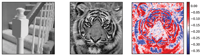
Figure 18-9: Left: We present our tiny autoencoder trained on just the tiger with an image of a stairway. Middle: The output is the tiger! Right: The difference between the output image and the original tiger.
The error bar on the right of Figure 18-9 shows that our errors are much larger than those of Figure 18-8, but the tiger still looks a lot like the original.
Let’s make a real stress test of the idea that the network is mostly relying on the bias values. We can feed the autoencoder an input image that is zero everywhere. Then it has no input values to work with, and only the bias values contribute to the output. Figure 18-10 shows the result.
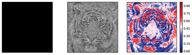
Figure 18-10: When we give our tiny autoencoder a field of pure black, it uses the bias values to give us back a low quality, but recognizable, version of the tiger. Left: The black input. Middle: The output. Right: The difference between the output and the original tiger. Note that the range of differences runs from 0 to almost 1, unlike Figure 18-9 where they ran from about −0.4 to 0.
No matter what input we give to this network, we will always get back some version of the tiger as output. The autoencoder has trained itself to produce the tiger every time.
A real test of this autoencoder would be to teach it a bunch of images and see how well it compresses them. Let’s try again with a set of 25 photographs, shown in Figure 18-11.
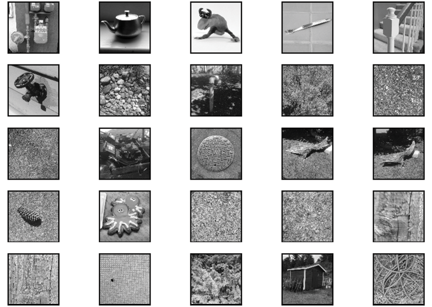
Figure 18-11: The 25 photographs that we used, in addition to the tiger, to train our tiny autoencoder. Each image was rotated by 90 degrees, 180 degrees, and 270 degrees during training.
We made the database larger by training not just on each image, but also on each image rotated by 90 degrees, 180 degrees, and 270 degrees. Our training set was the tiger (and its three rotations) and the 100 images of Figure 18-11 with rotations, for a total of 104 images.
Now that the system is trying to remember how to represent all 104 of these pictures with just 20 numbers, it should be no surprise that it can’t do a very good job. Figure 18-12 shows what this autoencoder produces when we ask it to compress and decompress the tiger.

Figure 18-12: We trained our autoencoder of Figure 18-6 with the 100 images of Figure 18-11 (each image plus its rotated versions), along with the four rotations of the tiger. Using this training, we gave it the tiger on the left, and it produced the output in the middle.
Now that the system isn’t allowed to cheat, the result doesn’t look like a tiger at all, and everything makes sense again. We can see a little bit of four-way rotational symmetry in the result, owing to our training on the rotated versions of the input images. We could do better by increasing the number of neurons in the bottleneck, or latent, layer. But since we want to compress our inputs as much as possible, adding more values to the bottleneck should be a last resort. We’d rather do the best possible job we can with as few values as we can get away with.
Let’s try to improve the performance by considering a more complex architecture than just the two dense layers we’ve been using so far.
A Better Autoencoder
In this section, we’ll explore a variety of autoencoder architectures. To compare them, we’ll use the MNIST database we saw in Chapter 17. To recap, this is a big, free database of hand-drawn, grayscale digits from 0 to 9, saved at a resolution of 28 by 28 pixels. Figure 18-13 shows some typical digit images from the MNIST dataset.
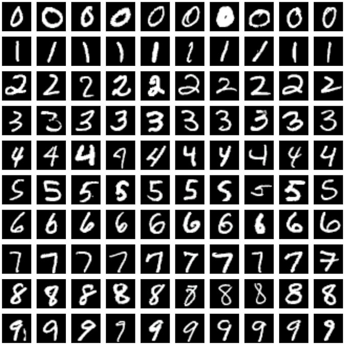
Figure 18-13: A sampling of the handwritten digits from the MNIST dataset
To run our simple autoencoder on this data, we need to change the size of the inputs and outputs of Figure 18-6 to fit the MNIST data. Each image has 28 × 28 = 784 pixels. Thus, our input and output layer now needs 784 elements instead of 10,000. Let’s flatten the 2D image into a single big list before we feed it to the network and leave the bottleneck at 20. Figure 18-14 shows the new autoencoder. In this diagram, as well as those to come, we won’t draw the flatten layer at the start, or the reshaping layer at the end that “undoes” the flattening and turns the list of 784 numbers back into a 28 by 28 grid.
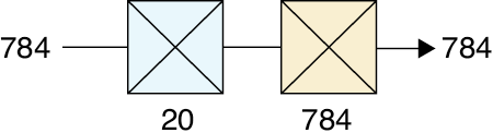
Figure 18-14: Our two-layer autoencoder for MNIST data
Let’s train this for 50 epochs (that is, we run through all 60,000 training examples 50 times). Some results are shown in Figure 18-15.
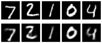
Figure 18-15: Running five digits from the MNIST dataset through our trained autoencoder of Figure 18-14, which uses 20 latent variables. Top row: Five pieces of input data. Bottom row: The reconstructed images.
Figure 18-15 is pretty amazing. Our two-layer network learned how to take each input of 784 pixels, squash it down to just 20 numbers, and then blow it back up to 784 pixels. The resulting digits are blurry, but recognizable.
Let’s try reducing the number of latent variables down to 10. We expect things are going to look a lot worse. Figure 18-16 shows that they are indeed worse.

Figure 18-16: Top row: The original MNIST images. Bottom row: The output of our autoencoder using 10 latent variables.
This is getting pretty bad. The 2 seems to be turning into a 3 with a bite taken out of it, and the 4 seems to be turning into a 9. But that’s what we get for crushing these images down to 10 numbers. That’s just not enough to enable the system to do a good job of representing the input.
The lesson is that our autoencoder needs to have both enough computational power (that is, enough neurons and weights) to figure out how to encode the data, and enough latent variables to find a useful compressed representation of the input.
Let’s see how deeper models perform. We can build the encoder and decoder with any types of layers we like. We can make deep autoencoders with lots of layers, or shallow ones with only a few, depending on our data. For now, let’s continue using fully connected layers, but let’s add some more of them to create a deeper autoencoder. We’ll construct the encoder stage from several hidden layers of decreasing size until we reach the bottleneck, and then we’ll build a decoder from several more hidden layers of increasing size until they reach the same size as the input.
Figure 18-17 shows this approach where now we have three layers of encoding and three of decoding.

Figure 18-17: A deep autoencoder built out of fully connected (or dense) layers. Blue icons: A three-layer encoder. Beige icons: A three-layer decoder.
We often build these fully connected layers so that their numbers of neurons decrease (and then increase) by a multiple of two, as when we go between 512 and 256. That choice often works out well, but there’s no rule enforcing it.
Let’s train this autoencoder just like the others, for 50 epochs. Figure 18-18 shows the results.
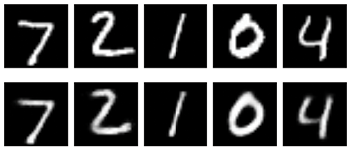
Figure 18-18: Predictions from our deep autoencoder of Figure 18-17. Top row: Images from the MNIST test set. Bottom row: Output from our trained autoencoder when presented with the test digits.
The results are just a little blurry, but they match the originals unambiguously. Compare these results to Figure 18-15, which also used 20 latent variables. These images are much clearer. By providing additional compute power to find those variables (in the encoder), and extra power in turning them back into images (in the decoder), we’ve gotten much better results out of our 20 latent variables.
Exploring the Autoencoder
Let’s look more closely at the results produced by the autoencoder network in Figure 18-17.
A Closer Look at the Latent Variables
We’ve seen that the latent variables are a compressed form of the inputs, but we haven’t looked at the latent variables themselves. Figure 18-19 shows graphs of the 20 latent variables produced by the network in Figure 18-17 in response to our five test images, and the images that the decoder constructs from them.

Figure 18-19: Top row: The 20 latent variables for each of our five images produced by the network in Figure 18-17. Bottom row: The images decompressed from the latent variables above them.
The latent variables shown in Figure 18-19 are typical, in the sense that latent variables rarely show any obvious connection to the input data from which they were produced. The network has found its own private, highly compressed form for representing its inputs, and that form often makes no sense to us. For example, we can see a couple of consistent holes in the graphs (in positions 4, 5, and 14), but there’s no obvious reason from this one set of images why those values are 0 (or nearly 0) for these inputs. Looking at more data would surely help, but the problem of interpretation remains, in general.
The mysterious nature of the latent variables is fine, because we rarely care about directly interpreting these values. Later on, we’ll play with the latent values, by blending and averaging them, but we won’t care about what these numbers represent. They’re just a private code that the network created during training that lets it compress and then decompress each input as well as possible.
The Parameter Space
Though we usually don’t care about the numerical values in the latent variables, it is still useful to get a feeling for what latent variables are produced by similar and different inputs. For example, if we feed the system two images of a seven that are almost the same, will the images be assigned almost the same latent variables? Or might they be wildly far apart?
To answer these questions, let’s continue with the simple deep autoencoder of Figure 18-17. But instead of making the last stage of the encoder a fully connected layer of 20 neurons, let’s drop that to merely two neurons, so we have just two latent variables. The point of this is that we can plot the two variables on the page as (x,y) pairs. Of course, if we generate images from just two latent variables, those images will come out extremely blurry, but it’s worth the exercise so we can see the structure of these simple latent variables.
In Figure 18-20 we encoded 10,000 MNIST images, found each image’s two latent variables, and then plotted them as a point. Each dot is color-coded for the label assigned to the image it came from. We say that an image like Figure 18-20 is a visualization of latent variable space, or more simply, latent space.

Figure 18-20: After training a deep autoencoder with only two latent variables, we show the latent variables assigned to each of 10,000 MNIST images.
There’s a lot of structure here! The latent variables aren’t being assigned numerical values totally at random. Instead, similar images are getting assigned similar latent variables. The 1’s, 3s, and 0s seem to fall into their own zones. Many of the other digits seem to be scrambled in the lower-left of the plot, getting assigned similar values. Figure 18-21 shows a close-up view of that region.
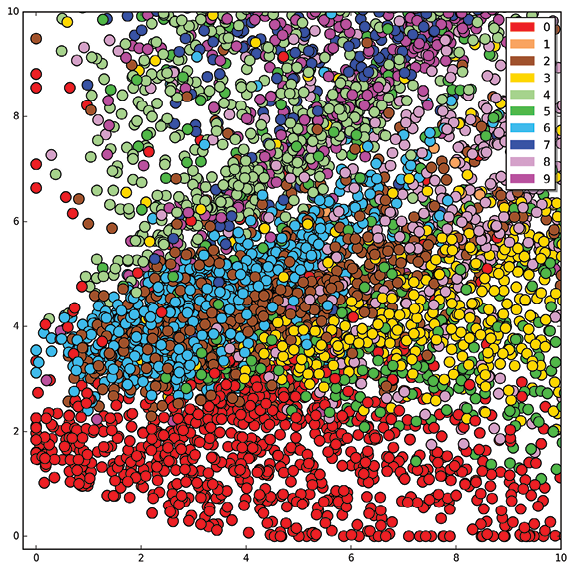
Figure 18-21: A close-up of the lower-left corner of Figure 18-20
It’s not a total jumble. The 0’s have their own band, and while the others are a bit mixed up, we can see they all seem to fall into well-defined zones.
Though we expect the images to be blurry, let’s make pictures from these 2D latent values. We can see from Figure 18-20 that the first latent variable (which we’re drawing on the X axis) takes on values from 0 to about 40, and the second latent variable (which we’re drawing on the Y axis) takes on values from 0 to almost 70.
Let’s make a square grid of decoded images, following the recipe in Figure 18-22. We can make a box that runs from 0 to 55 along each axis (that’s a little too short in Y, but a little too long in X). We can pick (x,y) points inside this grid, and then feed those two numbers to the decoder, producing a picture. Then we can draw the picture at that (x,y) position in a corresponding grid. We found that 23 steps on each axis produced a nice image that’s dense, but not overly so.
Figure 18-23 shows the result.

Figure 18-22: Making a grid of images by decoding (x,y) pairs from Figure 18-20 (and a little beyond). On the left, we select an (x,y) pair located at about (22,8). Then we pass these two numbers through the decoder, creating the tiny output image on the right.
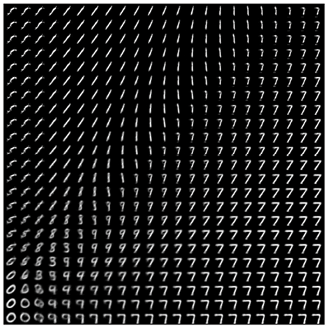
Figure 18-23: Images generated from latent variables in the range of Figure 18-22
The 1’s spray along the top, as expected. Surprisingly, the 7’s dominate the right side. As before, let’s look at the images in a close-up of the lower-left corner, shown in Figure 18-24.

Figure 18-24: Images from the close-up range of latent variables in Figure 18-23
The digits are frequently fuzzy, and they don’t fall into clear zones. This is not just because we’re using a very simple encoder, but because we’re encoding our inputs into just two latent variables. With more latent variables, things become more separated and distinct, but we can’t draw simple pictures of those high-dimensional spaces. Nevertheless, this shows us that even with an extreme compression down to just two latent variables, the system assigned those values in ways that grouped similar digits together.
Let’s look more closely at this space. Figure 18-25 shows the images produced by taking (x,y) values along four lines through the plot and feeding those to the decoder to produce images.
This confirms that the encoder assigned similar latent variables to similar images and seemed to build clusters of different images, with each variation of the image in its own region. That’s a whole lot of structure. As we increase our number of latent variables from this ridiculously small value of two, the encoder continues to produce clustered regions, but they become more distinct and there is less overlapping.
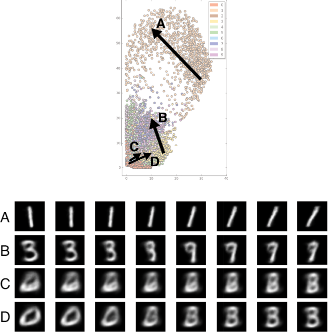
Figure 18-25: For each arrow, we took eight equally spaced steps from the start to the end, producing eight (x,y) pairs. The decoded images for these pairs are shown in the corresponding row.
Blending Latent Variables
Now that we’ve seen the structure inherent in the latent variables, we can put it to use. In particular, let’s blend some pairs of latent variables together and see if we get an intermediate image. In other words, let’s do parametric blending on the images, as we discussed earlier, where the latent variables are the parameters.
We actually did this in Figure 18-25 as we blended the two latent variables from one end of an arrow to the other. But there, we were using an autoencoder with just two latent variables, so it wasn’t able to represent the images very well. The results were mostly blurry. Let’s use some more latent variables so we can get a feeling for what this kind of blending, or interpolation, looks like in more complex models.
Let’s return to the six-layer version of our deep autoencoder of Figure 18-17, which has 20 latent variables. We can pick out pairs of images, find the latent variables for each one, and then simply average each pair of latent variables. That is, we have a list of 20 numbers for the first image (its latent variables) and a list of 20 numbers for the second image. We blend the first number in each list together, then the second number in each list, and so on, until we have a new list of 20 numbers. This is the new set of latent variables that we hand to the decoder, which produces an image.
Figure 18-26 shows five pairs of images blended this way.
As we expect, the system isn’t simply blending the images with content blending (like we did for the cow and zebra in Figure 18-1). Instead, the autoencoder is producing intermediate images that have qualities of both inputs.

Figure 18-26: Examples of blending latent variables in our deep autoencoder. Top row: Five images from the MNIST dataset. Middle row: Five other images. Bottom row: The image resulting from averaging the latent variables of the two images directly above, and then decoding.
These results aren’t absurd. For example, in the second column, the blend between a 2 and 4 looks like a partial 8. That makes sense. Figure 18-23 shows us that the 2s, 4s, and 8s are close together in the diagram with only 2 latent variables, so it’s reasonable that they could still be near one another in a 20-dimensional diagram with 20 latent variables.
Let’s look at this kind of blending of latent variables more closely. Figure 18-27 shows three new pairs of digits with six equally spaced steps of interpolation.

Figure 18-27: Blending the latent variables. For each row, we blend between the leftmost and rightmost sets of latent variables.
The far left and right of each row are images from the MNIST data. We found the 20 latent variables for each endpoint, created six equally spaced blends of those latent variables, and then ran those blended latents through the decoder. The system is trying to move from one image to another, but it’s not producing very reasonable intermediate digits. Even when going from a 5 to a 5 in the middle row, the intermediate values almost break up into two separate pieces before rejoining. Some of the blends near the middle of the top and bottom rows don’t look like any digits at all. Although the ends are recognizable, the blends fall apart very quickly. Blending latent parameters in this autoencoder smoothly changes the image from one digit to another, but the in-betweens are just weird shapes, rather than some kind of blended digits. We’ve seen that sometimes this is due to moving through dense regions where similar latent variables encode different digits. A bigger problem is conceptual. These examples may not even be wrong, since it’s not clear what a digit that’s partly 0 and partly 1 should look like, were we able to make one. Maybe the 0 should get thinner? Maybe the 1 should curl up into a circle? So although these blends don’t look like digits, they’re reasonable results.
Some of these interpolated latent values can land in regions of latent space where there’s no nearby data. In other words, we’re asking the decoder to reconstruct an image from values of latent variables that don’t have any nearby neighbors in latent space. The decoder is producing something, and that output has some qualities of the nearby regions, but the decoder is essentially guessing.
Predicting from Novel Input
Let’s try to use this deep autoencoder trained on MNIST data to compress and then decompress our tiger image. We will shrink the tiger to 28 by 28 pixels to match the network’s input size, so it’s going to look very blurry.
The tiger is like nothing the network has ever seen before, so it’s completely ill-equipped to deal with this data. It tries to “see” a digit in the image and produces a corresponding output. Figure 18-28 shows the results.
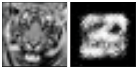
Figure 18-28: Encoding and then decoding a 28 by 28 version of our tiger of Figure 18-8 with our deep autoencoder of 20 latent variables, trained on the MNIST handwritten digit dataset
It looks like the algorithm has tried to find a spot that combines several different digits. The splotch in the middle isn’t much of a match to the tiger, but there’s no reason it should be.
Using information learned from digits to compress and decompress a tiger is like trying to build a guitar using parts taken from pencil sharpeners. Even if we do our best, the result isn’t likely to be a good guitar. An autoencoder can only meaningfully encode and decode the type of data it’s been trained on because it created meaning for the latent variables only to represent that data. When we surprise it with something completely different, it does its best, but it’s not going to be very good.
There are several variations on the basic autoencoder concept. Since we’re working with images, and convolution is a natural approach for that kind of data, let’s build an autoencoder using convolution layers.
Convolutional Autoencoders
We said earlier that our encoding and decoding stages could contain any kind of layers we wanted. Since our running example uses image data, let’s use convolutional layers. In other words, let’s build a convolutional autoencoder.
We will design an encoder to use several layers of convolution to scale down the original 28 by 28 MNIST image in stages until it’s just 7 by 7. All of our convolutions will use 3 by 3 filters, and zero-padding. As shown in Figure 18-29, we start with a convolution layer with 16 filters and follow it by a maximum pooling layer with a 2 by 2 cell, giving us a tensor that is 14 by 14 by 16 (we could have used striding during convolution, but we’ve separated the steps here for clarity). Then we apply another convolution, this time with 8 filters, and follow that with pooling, producing a tensor that’s 7 by 7 by 8. The final encoder layer uses three filters, producing a tensor that’s 7 by 7 by 3 at the bottleneck. Thus, our bottleneck represents the 768 inputs with 7 × 7 × 3 = 147 latent variables.
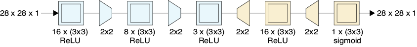
Figure 18-29: The architecture of our convolutional autoencoder. In the encoding stage (blue), we have three convolutional layers. The first two layers are each followed by a pooling layer, so by the end of the third convolutional layer, we have an intermediate tensor of shape 7 by 7 by 3. The decoder (beige) uses convolution and upsampling to grow the bottleneck tensor back into a 28 by 28 by 1 output.
Our decoder runs the process in reverse. The first upsampling layer produces a tensor that’s 14 by 14 by 3. The following convolution and upsampling gives us a tensor that’s 28 by 28 by 16, and the final convolution produces a tensor of shape 28 by 28 by 1. As before, we’re leaving out the flattening step at the start and the reshaping step at the end.
Since we’ve got 147 latent variables, along with the power of the convolutional layers, we should expect better results than with our previous autoencoder of just 20 latent variables. We trained this network for 50 epochs, just as before. The model was still improving at that point, but we stopped at 50 epochs for the sake of comparison with the previous models.
Figure 18-30 shows five examples from the test set and their decompressed versions after running through our convolutional autoencoder.
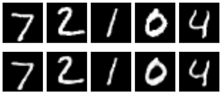
Figure 18-30: Top row: Five elements from the MNIST test set. Bottom row: The images produced by our convolutional autoencoder given the image above it as input.
These results are pretty great. The images aren’t identical, but they’re very close.
Just for fun, let’s try giving the decoder step nothing but noise. Since our latent variables are a tensor of size 7 by 7 by 3, our noise values need to be a 3D volume of the same shape. Rather than try to draw such a block of numbers, we will just show the topmost 7 by 7 slice of the block. Figure 18-31 shows the results.

Figure 18-31: Images produced by handing an input tensor of random values to the decoder stage of our convolutional neural network
This just produces randomly splotchy images, which seems a fair output for a random input.
Blending Latent Variables
Let’s blend the latent variables in our convolutional autoencoder and see how it goes. In Figure 18-32 we show our grid using the same images as in Figure 18-26. We find the latent variables for each image in the top two rows, blend them equally, and then decode the interpolated variables to create the bottom row.
The results are pretty gloppy, though some have a feeling of being a mix of the images from the rows above. Again, we shouldn’t be too surprised, since it’s not clear what a digit halfway between, say, 7 and 3 ought to look like.

Figure 18-32: Blending latent variables in the convolutional autoencoder. Top two rows: Samples from the MNIST dataset. Bottom row: The result of an equal blend of the latent variables from each of the above images.
Let’s look at multiple steps along the way in the same three blends that we used before in Figure 18-27. The results are shown in Figure 18-33.
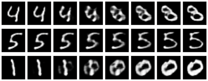
Figure 18-33: Blending the latent variables of two MNIST test images and then decoding
The left and right ends of each row are images created by encoding and decoding an MNIST image. In between are the results of blending their latent variables and then decoding. This isn’t looking a whole lot better than our simpler autoencoder. So just because we have more latent variables, we still run into trouble when we try to reconstruct using inputs that are too unlike the samples that the system was trained on. For example, in the top row we didn’t train on any input images that were in some way “between” a 4 and 3, so the system didn’t have any good information on how to produce images from latent values representing such a thing.
Predicting from Novel Input
Let’s repeat our completely unfair test by giving the low-resolution tiger to our convolutional neural net. The results are shown in Figure 18-34.
If we squint, it looks like the major dark regions around the eyes, the sides of the mouth, and the nose, have been preserved. Maybe. Or maybe that’s just imagination.
As with our earlier autoencoder built from fully connected layers, our convolutional autoencoder is trying to find a tiger somewhere in the latent space of digits. We shouldn’t expect it to do well.
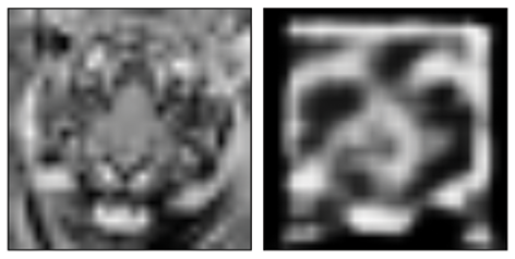
Figure 18-34: The low-resolution tiger we applied to our convolutional autoencoder, and the result. It’s not very tiger-like.
Denoising
A popular use of autoencoders is to remove noise from samples. A particularly interesting application is to remove the speckling that sometimes appears in computer-generated images (Bako et al. 2017; Chaitanya 2017). These bright and dark points, which can look like static, or snow, can be produced when we generate an image quickly, without refining all the results.
Let’s see how to use an autoencoder to remove bright and dark dots in an image. We will use the MNIST dataset again, but this time, we’ll add some random noise to our images. At every pixel, we pick a value from a Gaussian distribution with a mean of 0, so we get positive and negative values, add them in, and then clip the resulting values to the range 0 to 1. Figure 18-35 shows some MNIST training images with this random noise applied.
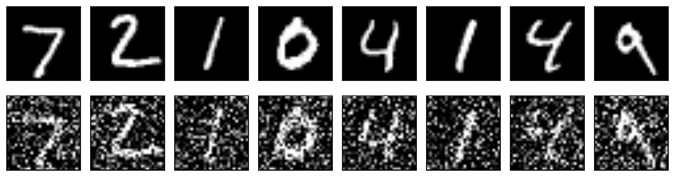
Figure 18-35: Top: MNIST training digits. Bottom: The same digits but with random noise.
Our goal is to give our trained autoencoder the noisy versions of the digits in the bottom row of Figure 18-35 and have it return cleaned-up versions like the top row of in Figure 18-35. Our hope is that the latent variables won’t encode the noise, so we’ll get back just the digits.
We’ll use an autoencoder with the same general structure as Figure 18-29, though with different numbers of filters (Chollet 2017). Figure 18-36 shows the architecture.
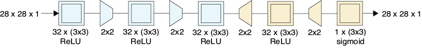
Figure 18-36: A denoising autoencoder
To train our autoencoder, we’ll give it noisy image inputs and their corresponding clean, noise-free versions as the targets we want it to produce. We’ll train with all 60,000 images for 100 epochs.
The tensor at the end of the decoding step in Figure 18-35 (that is, after the third convolution) has size 7 by 7 by 32, for a total of 1,568 numbers. So our “bottleneck” in this model is twice the size of the input. That would be bad if our goal was compression, but here we’re trying to remove noise, so minimizing the number of latent variables isn’t as much of a concern.
How well does it perform? Figure 18-37 shows some of the noisy inputs and the autoencoder’s outputs. It cleaned up the pixels very well, giving us great-looking results.

Figure 18-37: Top row: Digits with noise added. Bottom row: The same digits denoised by our model of Figure 18-36.
In Chapter 16, we discussed that explicit upsampling and downsampling layers are falling out of favor, replaced by striding and transposed convolution. Let’s follow that trend to simplify our model of Figure 18-36 to make Figure 18-38, which is now made up of nothing but a sequence of five convolution layers. The first two convolutions use striding to replace explicit downsampling layers, and the last two layers use repetition instead of explicit upsampling layers. Recall that we’re assuming zero-padding in each convolution layer.

Figure 18-38: The autoencoder of Figure 18-36 but using downsampling and upsampling inside the convolution layers, as shown by the wedges attached to the convolution icons
Figure 18-39 shows the results.
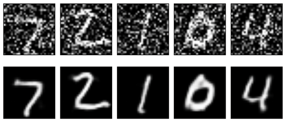
Figure 18-39: The results of our denoising model of Figure 18-38
The outputs are quite close, though there are small differences (for example, look at the bottom-left of the 0). The first model, Figure 18-36, with explicit layers for upsampling and downsampling, took roughly 300 seconds per epoch on a late 2014 iMac with no GPU support. The simpler model of Figure 18-38 took only about 200 seconds per epoch so it shaved off about one-third of the training time.
It would require a more careful problem statement, testing, and review of the results to decide if either of these models produces better results than the other for this task.
Variational Autoencoders
The autoencoders we’ve seen so far have tried to find the most efficient way to compress an input so that it can later be re-created. A variational autoencoder (VAE) shares the same general architecture as those networks but does an even better job of clumping the latent variables and filling up the latent space.
VAEs also differ from our previous autoencoders because they have some unpredictability. Our previous autoencoders were deterministic. That is, given the same input, they always produce the same latent variables, and those latent variables always then produce the same output. But a VAE uses probabilistic ideas (that is, random numbers) in the encoding stage; if we run the same input through the system multiple times, we get a slightly different output each time. We say that a VAE is nondeterministic.
As we look at the VAE, let’s continue to phrase our discussion in terms of images (and pixels) for concreteness, but like all of our other machine learning algorithms, a VAE can be applied to any kind of data: sound, weather, movie preferences, or anything else we can represent numerically.
Distribution of Latent Variables
In our previous autoencoders we didn’t impose any conditions on the structure of the latent variables. In Figure 18-20, we saw that a fully connected encoder seemed to naturally group the latent variables into blobs radiating to the right and upward from a common starting point at (0,0). That structure wasn’t a design goal. It just came out that way as a result of the nature of the network we built. The convolutional network in Figure 18-38 produces similar results when we reduce the bottleneck to two latent variables, shown here in Figure 18-40.
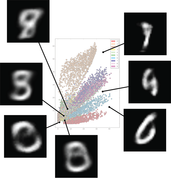
Figure 18-40: The latent variables produced by the convolutional autoencoder of Figure 18-38 with a bottleneck of two latent variables. These samples are drawn from both densely mixed and sparse regions.
Figure 18-40 shows decoded images generated from latent variables chosen from both dense and sparse regions.
In Figure 18-22 we saw that we can pick any pair of latent variables and run those values through a decoder to make an image. Figure 18-40 shows that if we pick these points in the dense zones, or the unoccupied zones, we often get back images that don’t look like digits. It would be great if we could find a way to set things up so that any pair of inputs always (or almost always) produces a good-looking digit.
Ideally, it would be great if each digit had its own zone, the zones didn’t overlap, and we didn’t have any big, empty spaces. There’s not much we can do about filling in empty zones, since those are places where we just don’t have input data. But we can try to break apart the mixed zones so that each digit occupies its own region of the latent space.
Let’s see how a variational autoencoder does a good job of meeting these goals.
Variational Autoencoder Structure
As so often happens with good ideas, the VAE was invented simultaneously but independently by at least two different groups (Kingma and Welling 2014; Rezende, Mohamed, and Wierstra 2014). Understanding the technique in detail requires working through some math (Dürr 2016), so instead, let’s take an approximate and conceptual approach. Because our intent is to capture the gist of the method rather than its precise mechanics, we will skip some details and gloss over others.
Our goal is to create a generator that can take in random latent variables and produce new outputs that are reasonably like inputs that had similar latent values. Recall that the distribution of the latent variables is created together by the encoder and decoder during training. During that process, in addition to making sure the latent variables let us reconstruct the inputs, we also desire that the latent variables obey three properties.
First, all of the latent variables should be gathered into one region of latent space so we know what the ranges should be for our random values. Second, latent variables produced by similar inputs (that is, images that show the same digit) should be clumped together. Third, we want to minimize empty regions in the latent space.
To satisfy these criteria, we can use a more complicated error term that punishes the system when it makes latent samples that don’t follow the rules. Since the whole point of learning is to minimize the error, the system will learn how to create latent values that are structured the way we want. The architecture and the error term are designed to work together. Let’s see what that error term looks like.
Clustering the Latent Variables
Let’s first tackle the idea of keeping all latent variables together in one place. We can do that by imposing a rule, or constraint, which we build into the error term.
Our constraint is that the values for each latent variable, when plotted, come close to forming a unit Gaussian distribution. Recall from Chapter 2 that a Gaussian is the famous bell curve, illustrated in Figure 18-41.

Figure 18-41: A Gaussian curve
When we place two Gaussians at right angles to one another, we get a bump above the plane, as in Figure 18-42.
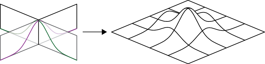
Figure 18-42: In 3D, we can place two Gaussians at right angles. Together, they form a bump over the plane.
Figure 18-42 shows a 3D visualization of a 2D distribution. We can create an actual 3D distribution by including another Gaussian on the Z axis. If we think of the resulting bump as a density, then this 3D Gaussian is like a dandelion puff, which is dense in the center but becomes sparser as we move outward.
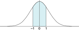
Figure 18-43: A Gaussian is described by its mean (the location of its center), and its standard deviation (the symmetrical distance that contains about 68 percent of its area). Here we have a center of 0, and a standard deviation of 1.
By analogy, we can imagine a Gaussian of any number of dimensions, just by saying that each dimension’s density follows a Gaussian curve on its axis. And that’s what we do here. We tell the VAE to learn values for the latent variables so that, when we look at the latent variables for lots of training samples and we count up how many times each value occurs, every variable’s counts form a distribution like a Gaussian that has its mean (or center) at 0, and a standard deviation (that is, its spread) of 1, as in Figure 18-43. Recall from Chapter 2 that this means that about 68 percent of the values we produce for this latent variable fall between −1 and 1.
When we’re done training, we know that our latent variables will be distributed according to this pattern. If we pick new values to feed to the decoder, and we select them from this distribution (where we’re more likely to pick each value near its center and within the bulk of its bump rather than off to the edges), we are likely to generate sets of latent values that are near values we learned from the training set, and thus we can create an output that is also like the training set. This naturally also keeps the samples together in the same area, since they’re all trying to match a Gaussian distribution with a center of 0.
Getting the latent variables to fall within unit Gaussians, as shown in Figure 18-43, is an ideal we rarely achieve. There’s a tradeoff between how well the variables match Gaussians and how accurate the system can be in re-creating inputs (Frans 2016). The system automatically learns that tradeoff during the training session, striving to keep the latents Gaussian-like while also reconstructing the inputs well.
Clumping Digits Together
Our next goal is getting the latent values of all images with the same digits to clump together. To do this, let’s use a clever trick that involves some randomness. It’s a bit subtle.
Let’s start by assuming that we’ve already achieved this goal. We will see what this implies from a particular point of view, and that will tell us how to actually bring it about. For example, we’re assuming that every set of latent variables for an image of, say, the digit 2 is near every other set of latent variables for images of the digit 2. We can do even better, though. Some 2s have a loop in the lower-left corner. So, in addition to having all the 2s clumped together, we can keep all the 2s with loops together and all the 2s without loops together, and the region between those clumps is filled with the latent variables of 2s that sort-of have a loop, as in Figure 18-44.
Now let’s carry this idea to its limit. Whatever the shape and style and line thickness and tilt and so on of every image that’s labeled a 2, we’ll assign that image latent variables that are near other images labeled 2 that show about the same shape and style. We can gather together all the 2s with a loop and all those without, all those drawn with straight lines and all those drawn with curves, all those with a thick stroke and all those with a thin one, all the 2s that are tall, and so on. That’s the major value of using lots of latent variables: they let us clump together all of the different combinations of these features, which wouldn’t be possible in just two dimensions. In one place we have thin straight no-loop 2s, another region has thick curved no-loop 2s, and so on, for every combination.

Figure 18-44: A grid of 2s organized so that neighbors are all like one another. We want the latent variables for these 2s to follow roughly this kind of structure.
If we had to identify all of these features ourselves, this scheme wouldn’t be very practical. But a VAE not only learns the different features, it automatically creates all the different groupings for us as it learns. As usual, we just feed in images and the system does all the rest of the work.
This “nearness” criterion is measured in latent space, where there’s one dimension for each latent variable. In two dimensions, each set of latent variables creates a point on the plane, and their distance (or “nearness”) is the length of the line between them. We can generalize this idea to any number of dimensions, so we can always find the distance between two sets of latent variables, even if each one has 30 or even 300 values: we just measure the length of the line that joins them.
We want the system to clump together similar-looking inputs. But recall that we also want each latent variable to form a Gaussian distribution. These two criteria can come into conflict. By introducing some randomness, we can tell the system to “usually” clump the latent variables for similar input, and “usually” also distribute those variables along a Gaussian curve. Let’s see how randomness lets us make that happen.
Introducing Randomness
Suppose that our system is given an input of an image of the digit 2, and as usual, the encoder finds the latent variables for it. Before we hand these to the decoder to produce an output image, let’s add a little randomness to each of the latent variables and pass those modified values to the decoder, as in Figure 18-45.

Figure 18-45: One way to add randomness to the output of the encoder is to add a random value to each latent variable before passing them to the decoder.
Because we’re assuming that all of the examples of the same style are clumped together, the output image we generate from the perturbed latent variables will be similar to (but different from) our input, and thus the error that measures the difference between the images will also be low. Then we can make lots of new 2’s that are like the input 2, just by adding different small random numbers to the same set of latent values.
That’s how it works once the clumping has already been done. To get the clumping done in the first place, all we have to do is give the network a big error score during training when this perturbed output doesn’t come very close to matching the input. Because the system wants to minimize the error, it learns that latent values that are close to the input’s original latent values should produce images that are close to the input image. As a result, the latent values for similar inputs get clumped together, just as we desired.
But we took a shortcut just now that we can’t follow in practice. If we just add random numbers as in Figure 18-45, we won’t be able to use the backpropagation algorithm we saw in Chapter 14 to train the model. The problem comes about because backpropagation needs to compute the gradients flowing through the network, but the mathematics of an operation like Figure 18-45 don’t let us calculate the gradients the way we need to. And without backpropagation, our whole learning process disappears in a puff of smoke.
VAEs use a clever idea to get around this problem, replacing the process of adding random values with a similar idea that does about the same job, but which lets us compute the gradient. It’s a little bit of mathematical substitution that lets backpropagation work again. This is called the reparameterization trick. (As we’ve seen a few times, mathematicians sometimes use the word trick as a compliment when referring to a clever idea.)
It’s worth knowing about this trick because it often comes up when we’re reading about VAEs (there are other mathematical tricks involved, but we won’t go into them). The trick is this: instead of just picking a random number from thin air for each latent variable and adding it in, as in Figure 18-45, we draw a random variable from a probability distribution. That value now becomes our latent variable (Doersch 2016). In other words, rather than start with a latent value and then add a random offset to it to create a new latent value, we use the latent value to control a random number generation process, and the result of that process becomes the new latent value.
Recall from Chapter 2 that a probability distribution can give us random numbers, where some are more likely than others. In this case, we use a Gaussian distribution. This means that when we ask for a random value, we’re most likely to get a number near where the bump is high, and we’re less and less likely to get numbers that are farther away from the center of the bump.
Since each Gaussian requires a center (the mean) and a spread (the standard deviation), the encoder produces this pair of numbers for each latent variable. If our system has eight latent variables, then the encoder produces eight pairs of numbers: the center and spread for a Gaussian distribution for each one. Once we have them, then for each pair of values, we pick a random number from the distribution they define, and that’s the value of the latent variable that we then give to the decoder. In other words, we create a new value for each latent variable that’s pretty close to where it was, but has some randomness built in. The restructuring of the perturbation process lets us apply backpropagation to the network.
Figure 18-46 shows the idea.
The structure of our autoencoder, as shown in Figure 18-46, requires the network to split after the computation of the latent value. Splitting is a new technique for our repertoire of deep learning architectures: it just takes a tensor and duplicates it, sending the two copies to two different subsequent layers. After the split, we use one layer to compute the center of the Gaussian and one to compute the spread. We sample this Gaussian and that gives us our new latent value.
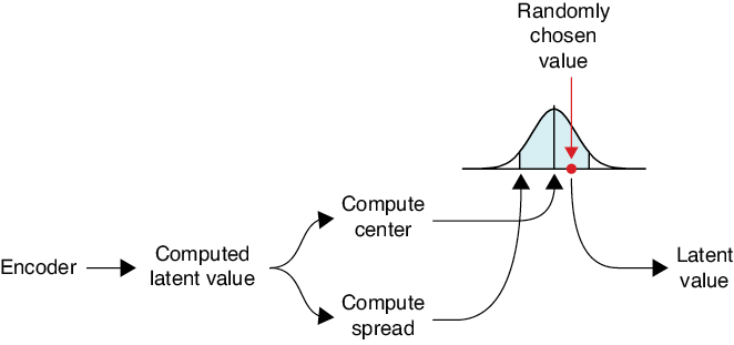
Figure 18-46: We use the computed latent value to get the center and spread of a Gaussian bump. We pick a number from that bump, and that becomes our new latent value.
To apply our sampling idea of Figure 18-46, we create a Gaussian for each latent variable and sample it. Then we feed all of the new latent values into a merge or combination layer, which simply places all of its inputs one after the other to form a single list (in practice, we often combine the sampling and merging steps together into one layer). Figure 18-47 shows how we’d process a latent vector with three values.
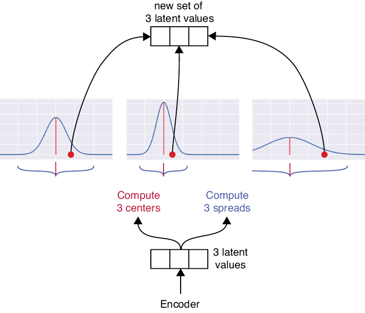
Figure 18-47: Picturing the split-and-combine sampling step of a VAE for three latent variables
In Figure 18-47, the encoder ends with three latent variables, and for each one, we compute a center and spread. Those three different Gaussian bumps are then randomly sampled, and those selected values are merged, or combined, to form the final latent variables computed for that input. These variables are the output of the encoder section.
During the learning process, the network learns what the centers and spreads should be for each Gaussian.
This operation is why we said earlier that each time we send a sample into a trained VAE (that is, after learning is done), we get back a slightly different result. The encoder is deterministic up to and including the split. But then the system picks a random value for each latent variable from its Gaussian, and those are different each time.
Exploring the VAE
Figure 18-48 shows the architecture of a fully connected VAE. It’s just like our deep autoencoder built from fully connected layers of Figure 18-17, but with two changes (we chose fully connected layers rather than convolution layers for simplicity).
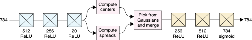
Figure 18-48: The architecture of our VAE for MNIST data. There are 20 latent values.
The first change is that we now we have the split-select-merge process at the end of the encoder. The second change is that we use our new loss, or error, function.
Another job we’ll assign to our new loss function is to measure the similarity between the fully connected layers of the encoding and decoding stages. After all, whatever the encoding stage is doing, we want the decoding stage to undo it.
The perfect way to measure this is with the Kullback–Leibler (or KL) divergence that we saw in Chapter 6. Recall that this measures the error we get from compressing information using an encoding that is different from the optimal one. In this case, we’re asserting that the optimal encoder is the opposite of the decoder, and vice versa. The big picture is that as the network tries to decrease the error, it is therefore decreasing the differences between the encoder and decoder, bringing them closer to mirroring each other (Altosaar 2020).
Working with the MNIST Samples
Let’s see what comes out of this VAE for some of our MNIST samples. Figure 18-49 shows the result.

Figure 18-49: Predictions from our VAE of Figure 18-48. Top row: Input MNIST data. Bottom row: Output of the variational autoencoder.
It’s no surprise that these are pretty good matches. Our network is using a lot of compute power to make these images! But as we have seen from its architecture, the VAE produces different outputs each time it sees the same image. Let’s take the image of the two from this test set and run it through the VAE eight times. The results are in Figure 18-50.

Figure 18-50: The VAE produces a different result each time it sees the same input. Top row: The input image. Middle row: The output from the VAE after processing the input eight times. Bottom row: The pixel by pixel differences between the input and each output. Increasing red means larger positive differences, increasing blue means larger negative differences.
These eight results from the VAE are similar to each other, but we can see obvious differences.
Let’s go back to our eight images from Figure 18-49 but add additional noise to the latent variables that come out of the encoder. That is, just before the decoder stage, we add some noise to the latent variables. This gives us a good test of how clumped-together the training images are in latent space.
Let’s try adding a random value that’s up to 10 percent of each latent variable’s amount. Figure 18-51 shows the result of adding this moderate amount of noise to the latent variables.

Figure 18-51: Adding 10 percent noise to the latent variables coming out of the VAE encoder. Top row: Input images from MNIST. Bottom row: The decoder output after adding noise to the latent variables produced by the encoder.
Adding noise doesn’t seem to change the images much at all. That’s great, because it’s telling us that these noisy values are still “near” the original inputs. Let’s crank up the noise, adding in a random number as much as 30 percent of the latent variable’s value. Figure 18-52 shows the result.

Figure 18-52: Perturbing the latent variables by up to 30 percent. Top row: The MNIST input images. Bottom row: The results from the VAE decoder.
Even with a lot of noise, the images still look like digits. For example, the 7 changes significantly, but it changes into a bent 7, not a random splotch.
Let’s try blending the parameters for our digits and see how that looks. Figure 18-53 shows the equal blends for the five pairs of digits we’ve seen before.

Figure 18-53: Blending latent variables in the VAE. Top and middle row: MNIST input images. Bottom row: An equal blend of the latent variables for each image, decoded.
The interesting thing here is that these are all looking roughly like digits (the leftmost image is the worst in terms of being a digit, but it’s still a coherent shape). That’s because there’s less unoccupied territory in latent space, so the intermediate values are less likely to land in a zone far from other data (and thus produce a strange, nondigit image).
Let’s look at some linear blends. Figure 18-54 shows the intermediate steps for the three pairs of digits we’ve seen before.
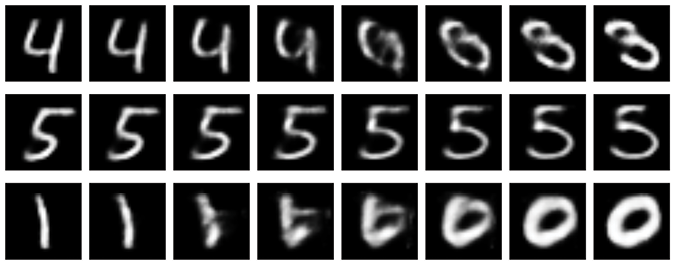
Figure 18-54: Linear interpolation of the latent variables in a VAE. The leftmost and rightmost image in each row are the output of the VAE for an MNIST sample. The images in between are decoded versions of the blended latent variables.
The 5 is looking great, moving through a space of 5s from one version to another. The top and bottom rows have plenty of images that aren’t digits. They might be passing through empty zones in latent space, but as we mentioned before, it’s not clear that these are wrong in any sense. After all, what should an image partly between a four and a three look like?
Let’s run our tiger through the system just for fun. Remember, this is a completely unfair thing to do, and we shouldn’t expect anything meaningful to come out. Figure 18-55 shows the result.
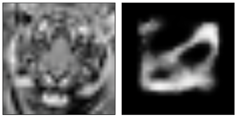
Figure 18-55: Running our low-resolution tiger through the VAE
The VAE created something with a coherent structure, but it’s not much like a digit.
Working with Two Latent Variables
For comparison to our other autoencoders, we trained our VAE with just 2 latent variables (rather than the 20 we’ve been using), and plotted them in Figure 18-56.
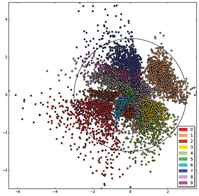
Figure 18-56: The placement of latent variables for 10,000 MNIST images from our VAE trained with two latent variables
This is a great result. The standard deviation of the Gaussian bump the latent variables are trying to stay within is represented here by a black circle, and it seems pretty well populated. The various digits are generally well clumped. There’s some confusion in the middle, but remember that this image uses just two latent variables. Curiously, the 2s seem to form two clusters. To see what’s going on, let’s make a grid of images that correspond to our two latent variables using the recipe shown in Figure 18-22, but using the latent variables of Figure 18-56. Let’s take the x and y values of each point on the grid and feed them to the decoder as though they were latent variables. Our range is −3 to 3 on each axis, like the circle in Figure 18-56. The result is Figure 18-57.
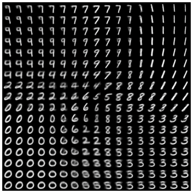
Figure 18-57: The output of the VAE treating the x and y coordinates as the two latent variables. Each axis runs from −3 to 3.
The 2s without a loop are grouped together near the lower middle, and the 2s with a loop are grouped in the middle left. The system decided that these were so different that they didn’t need to be near each other.
Looking over this figure, we can see how nicely the digits have been clumped together. This is a far more organized and uniform structure than we saw in Figure 18-23. In a few places the images get fuzzy, but even with just two latent variables, most of the images are digit-like.
Producing New Input
In Figure 18-58 we’ve isolated the decoder part of the VAE to use as a generator. For the moment, we’ll continue to use a version where we’ve reduced the 20 latent values to just 2.
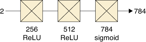
Figure 18-58: The decoder stage of our VAE
Since we have only two latent variables, we randomly picked 80 random (x,y) pairs from a circle centered at (0,0) with radius 3, fed them into the decoder, and gathered the resulting images together into Figure 18-59.
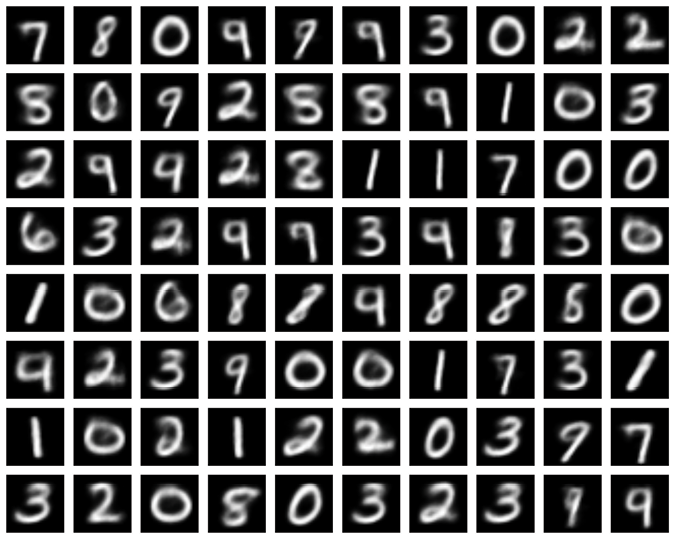
Figure 18-59: Images produced by the VAE decoder when presented with two random latent variables
These are looking pretty great for the most part. Some aren’t quite legible, but overall, most of the images are recognizable digits. Many of the mushiest shapes seem to have come from the boundary between the 8s and the 1s, leading to narrow and thin 8s.
Most of these digits are fuzzy, because we’re using only two latent variables. Let’s sharpen things up by training and then using a deeper VAE with more latent variables. Figure 18-60 shows our new VAE. This architecture is based on the MLP autoencoder that’s part of the Caffe machine-learning library (Jia and Shelhamer 2020; Donahue 2015). (Recall that MLP stands for multilayer perceptron, or a network built only out of fully connected layers.)
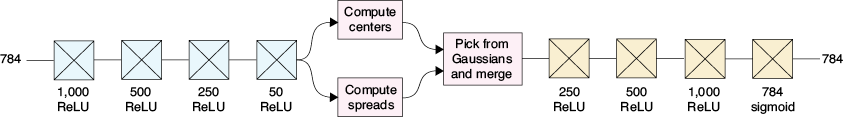
Figure 18-60: The architecture of a deeper VAE
We trained this system with 50 latent variables for 25 epochs and then generated another grid of random images. As before, we used just the decoder stage, shown in Figure 18-61.

Figure 18-61: We generate new output using just the decoder stage of our deeper VAE, feeding in 50 random numbers to produce images.
The results are in Figure 18-62.

Figure 18-62: Images produced by our bigger VAE when provided with random latent variables
These images have significantly crisper edges than the images in Figure 18-59. For the most part, we’ve generated entirely recognizable and plausible digits from purely random latent variables, though, as usual, some weird images that aren’t much like digits show up. These are probably coming from the empty zones between digits, or zones where different digits are near one another, causing oddball blends of the shapes.
Once our VAE has been trained, if we want to make more digit-like data, we can ignore the encoder and save the decoder. This is now a generator that we can use to create as many new digit-like images as we like. If we were to train the VAE on images of tractors, songbirds, or rivers, we could generate more of those types of images, too.
Summary
In this chapter we saw how autoencoders learn to represent a set of inputs with latent variables. Usually there are fewer of these latent variables than there are values in the input, so we say that the autoencoder compresses the input by forcing it through a bottleneck. Because some information is lost along the way, it’s a form of lossy compression.
By feeding latent values of our own choice directly into the second half of a trained autoencoder, we can view that set of layers as a generator, capable of producing new output data that is like the input, but wholly novel.
Autoencoders may be built using many kinds of layers. In this chapter, we saw examples of networks built from fully connected layers and convolution layers. We looked at the structure of 2D latent variables generated by a trained autoencoder built of fully connected layers, and found that it had a surprising amount of organization and structure. Picking new pairs of latents from a populated region of these latents and handing them to a generator usually produced an output that was blurry (because we had only two latent values), but plausibly like the input. We then looked at convolutional autoencoders, built primarily (or exclusively) with convolution layers.
We saw that we could blend latent variables, in essence creating a series of in-between latent variables between the endpoints. The more latent variables we used in our bottleneck, the better these interpolated outputs appeared. We then saw that an autoencoder can be trained to denoise the input, simply by telling it to generate the clean value of a noisy input. Finally, we looked at variational autoencoders, which do a better job of clumping similar inputs and filling up a region of the latent space, at the cost of introducing some randomization into the process.
Autoencoders are often used for denoising and simplifying datasets, but people have found creative ways to use them for many kinds of tasks, such as creating music and modifying input data to help networks learn better and faster (Raffel 2019).