In the previous chapter, we looked at dynamic programming where we knew the model dynamics p(s’, r| s, a), and this knowledge was used to “plan” the optimal actions. This is also known as the planning problem . In this chapter, we will shift our focus and look at learning problems , i.e., a setup where the model dynamics are not known. We will learn value and action-value functions by sampling, i.e., collecting experience by following some policy in the real world or by running the agent through a policy in simulation. There is another class of problems where we find the model-free approach more applicable. In some problems, it is easier to sample than to calculate the transition dynamics, e.g., consider solving a problem of finding the best policy to play a game like blackjack. There are many combinations to reach a score that depend on the cards seen so far and the cards still in the deck. It is almost impossible to calculate the exact transition probabilities from one state to another state but easy to sample states from an environment. To summarize, we use model-free methods when either we do not know the model dynamics or we know the model, but it is much more practical to sample than to calculate the transition dynamics.
In this chapter, we will look at two broad classes of model-free learning: Monte Carlo (MC) methods and temporal difference (TD) methods. We will first understand how policy evaluation works in a model-free setup and then extend our understanding to look at control, i.e., to find the optimal policy. We will also touch upon the important concept of bootstrapping and the exploration-versus-exploitation dilemma as well as off-policy versus on-policy learning. Initially, the focus will be to look at the MC and TD methods individually, after which we will look into additional concepts like n-step returns, importance sampling, and eligibility traces in a bid to combine the MC and TD methods into a common, more generic approach called TD(λ).
Estimation/Prediction with Monte Carlo
When we do not know the model dynamics, what do we do? Think back to a situation when you did not know something about a problem. What did you do in that situation? You experiment, take some steps, and find out how the situation responds. For example, say you want to find out if a die or a coin is biased or not. You toss the coin or throw the die multiple times, observe the outcome, and use that to form your opinion. In other words, you sample. The law of large numbers from statistics tell us that the average of samples is a good substitute for the averages. Further, these averages become better as the number of samples increase. If you look back at the Bellman equations in the previous chapter, you will notice that we had expectation operator E[•] in those equations; e.g., the value of a state being v(s) = E[Gt|St = s]. Further, to calculate v(s), we used dynamic programming requiring the transition dynamics p(s’, r | s, a). In the absence of the model dynamics knowledge, what do we do? We just sample from the model, observing returns starting from state S = s and until the end of the episode. We then average the returns from all episode runs and use that average as an estimate of vπ(s) for the policy π that the agent is following. This in a nutshell is the approach of Monte Carlo methods: replace expected returns with the average of sample returns.
There are a few points to note. MC methods do not require knowledge of the model. The only thing required is that we should be able to sample from it. We need to know the return of starting from a state until termination, and hence we can use MC methods only on episodic MDPs in which every run finally terminates. It will not work on nonterminating environments. The second point is that for a large MDP we can keep the focus on sampling only that part of the MDP that is relevant and avoid exploring irrelevant parts of the MDP. Such an approach makes MC methods highly scalable for very large problems. A variant of the MC method called Monte Carlo tree search (MCTS) was used by OpenAI in training a Go game-playing agent.
The third point is about Markov assumption; i.e., the past is fully encoded in the present state. In other words, knowing the present makes the future independent of the past. We talked about this property in Chapter 2. This property of Markov independence forms the basis of the recursive nature of Bellman equations where a state just depends on the successor state values. However, under the MC approach, we observe the full return starting from a state S and until termination. We are not depending on the value of successor states to calculate the current state value. There is no Markov property assumption being made here. A lack of Markov assumption in MC methods make them much more feasible for the class of MDPs known as POMDPs (for “partially observable MDP”). In a POMDP environment, we get only partial-state information, which is known as observation.
Moving on, let’s look at a formal way to estimate the state values for a given policy. We let the agent start a new episode and observe that the return from the time agent is in state S = s for the first time in that episode and until the episode ends. Many episode runs are carried out, and an average of return across episodes is taken as an estimate of vπ(S = s). This is known as the first-visit MC method . Please note that, depending on the dynamics, an agent may visit the same state S = s in some later step within the same episode before termination. However, in the first-visit MC method, we take the total return only from the first visit in an episode until the end of the episode. There is another variant in which we take the average of returns from every visit to that state until the end of the episode. This is known as the every-visit MC method .
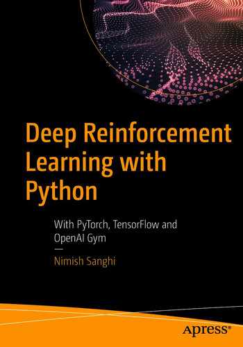
Backup diagram of MC methods as compared to Bellman equation–based DP backup
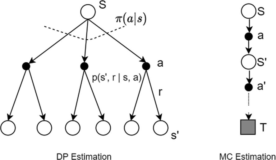
Let’s now look at the pseudocode for the first-visit version, which is given in Figure 4-2. We input the policy π that the agent is currently following. We initialize two arrays: one to hold the current estimate of V(s) and the second to hold the number of visits N(s) to a state S = s. Multiple episodes are executed, and we update V(s) as well as N(s) for the state agent visits in every episode, updating only for the first visit in the “first visit version” and updating for every visit in the “every visit version.” The pseudocode covers only the “first visit variant.” The “every visit” variant is easy to implement, just dropping the condition “Unless St appears in S0, S1, ….” As per the law of large numbers, the statistical law on which Monte Carlo simulations are based, V(s) will converge to true vπ(s) when the number of visits to each state goes to infinity.
First-visit MC prediction for estimating vπ(s). The pseudocode uses the online version to update the values as samples are received


![$$ V{(s)}_{n+1}=left[S{(s)}_n+G
ight]/N{(s)}_{n+1} $$](https://imgdetail.ebookreading.net/202109/3/9781484268094/9781484268094__9781484268094__files__images__502835_1_En_4_Chapter__502835_1_En_4_Chapter_TeX_Equh.png)
![$$ =left[V{(s)}_nast N{(s)}_n+G
ight]/N{(s)}_{n+1} $$](https://imgdetail.ebookreading.net/202109/3/9781484268094/9781484268094__9781484268094__files__images__502835_1_En_4_Chapter__502835_1_En_4_Chapter_TeX_Equi.png)
![$$ =V{(s)}_n+1/N{(s)}_{n+1}ast left[Ghbox{--} V{(s)}_n
ight] $$](https://imgdetail.ebookreading.net/202109/3/9781484268094/9781484268094__9781484268094__files__images__502835_1_En_4_Chapter__502835_1_En_4_Chapter_TeX_Equ1.png)
The difference [G – V(s)n] can be viewed as an error between the latest sampled value G and the current estimate V(s)n. The difference/error is then used to update the current estimate by adding 1/N ∗ error to the current estimate. As the number of visits increases, the new sample has increasingly low influence in revising the estimate of V(s). This is because the multiplication factor 1/N reduces to zero as N becomes very large.

The constant multiplication factor approach is more appropriate for problems that are nonstationary or when we want to give a constant weight to all the errors. A situation like this can happen when the old estimate Vn may not be very accurate.
MC Value Prediction Algorithm for Estimation
The code in Listing 4-1 is a straight implementation of the pseudocode in Figure 4-2. The code implements the online version of update as explained in equation (4.1), i.e., N[s]+=1; V[s]=V[s]+1/N[s]*(G-V[s]). The code also implements the “first-visit” version but can be converted to “every visit” with a very small tweak. We just need to drop the “if” check, i.e., “if s not in episode_states[:t]” to carry out the updates at every step.
To ensure convergence to the true state values, we need to ensure each state is visited enough times, being infinite in limit. As shown in the results at the end of the Python notebook, state values do not converge very well for 100 episodes. However, with 10,000 episodes, the values have converged well and match those produced with the DP method given in Listing 3-2.
Bias and Variance of MC Predication Methods
Let’s now look at the pros and cons of “first visit” versus “every visit.” Do both of them converge to the true underlying V(s)? Do they fluctuate a lot while converging? Does one converge faster to true value? Before we answer this question, let’s first review the basic concept of bias-variance trade-off that we see in all statistical model estimations, e.g., in supervised learning.
Bias refers to the property of the model to converge to the true underlying value that we are trying to estimate, in our case vπ(s). Some estimators are biased, meaning they are not able to converge to the true value due to their inherent lack of flexibility, i.e., being too simple or restricted for a given true model. At the same time, in some other cases, models have bias that goes down to zero as the number of samples grows.
Variance refers to the model estimate being sensitive to the specific sample data being used. This means the estimate value may fluctuate a lot and hence may require a large data set or trials for the estimate average to converge to a stable value.
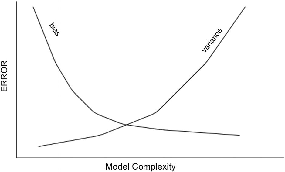
Bias variance trade-off. Model complexity is increasing toward the right on the x-axis. Bias starts off high when the model is restricted and drops off as the model becomes flexible. Variance shows a reverse trend with model complexity
Comparing “first visit” to “every visit,” first visit is unbiased but has high variance. Every visit has bias that goes down to zero as the number of trials increases. In addition, every visit has low variance and usually converges to the true value estimates faster than first visit.
Control with Monte Carlo
Let’s now talk about control in a model-free setup. We need to find the optimal policy in this setup without knowing the model dynamics. As a refresher, let’s look at the generalized policy iteration (GPI) that was introduced in Chapter 3. In GPI, we iterate between two steps. The first step is to find the state values for a given policy, and the second step is to improve the policy using greedy optimization. We will follow the same GPI approach for control under MC. We will have some tweaks, though, to account for the fact that we are in model-free world with no access/knowledge of transition dynamics.
In Chapter 3, we looked at state values, v(s). However, in the absence of transition dynamics, state values alone will not be sufficient. For the greedy improvement step, we need access to the action values, q(s, a). We need to know the q-values for all possible actions, i.e., all q(S = s, a) for all possible actions a in state S = s. Only with that information will we be able to apply a greedy maximization to pick the best action, i.e., argmaxaq(s, a).
We have another complication when compared to DP. The agent follows a policy at the time of generating the samples. However, such a policy may result in many state-action pairs never being visited, and even more so if the policy is a deterministic one. If the agent does not visit a state-action pair, it does not know all q(s, a) for a given state, and hence it cannot find the maximum q-value yielding an action. One way to solve the issue is to ensure enough exploration by exploring starts, i.e., ensuring that the agent starts an episode from a random state-action pair and over the course of many episodes covers each state-action pair enough times, in fact, infinite in limit.

Iteration between the two steps. The first step is evaluation to get the state-action values in sync with the policy being followed. The second step is that of policy improvement to do a greedy maximization for actions
The assumption of “exploring starts” is not very practical and efficient. It’s not practical, as in many scenarios, because the agent does not get to choose the start condition, e.g., while training a self-driving car. It’s not efficient, as it may not be feasible, and it may also be wasteful for the agent to visit each state-action pair infinite (in limit) times. We still need continued exploration for the agent to visit all the actions in the states that are visited by the current policy. This is achieved by using a ε-greedy policy.

The action with a maximum q-value gets picked with probability 1-ε from greedy max and ε/|A| as part of random exploration. All other actions are picked up with probability ε/|A|. As the agent learns over multiple episodes, the value of ε can be reduced slowly to zero to reach optimal greedy policy.
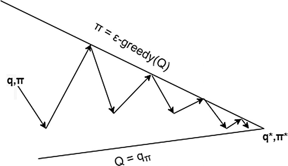
Iteration between the two steps. The first step is the MC prediction/evaluation for a single step to move the q-values in the direction of the current policy. The second step is that of policy improvement to do a ε-greedy maximization for actions
Combining all the previous tweaks, we have a practical algorithm for Monte Carlo–based control for optimal policy learning. This is called greedy in the limit with infinite exploration (GLIE). We will use the every-visit version in the q-value prediction step. But it takes a minor tweak, just like the one in MC prediction in Figure 4-6 to make it the first-visit variant.
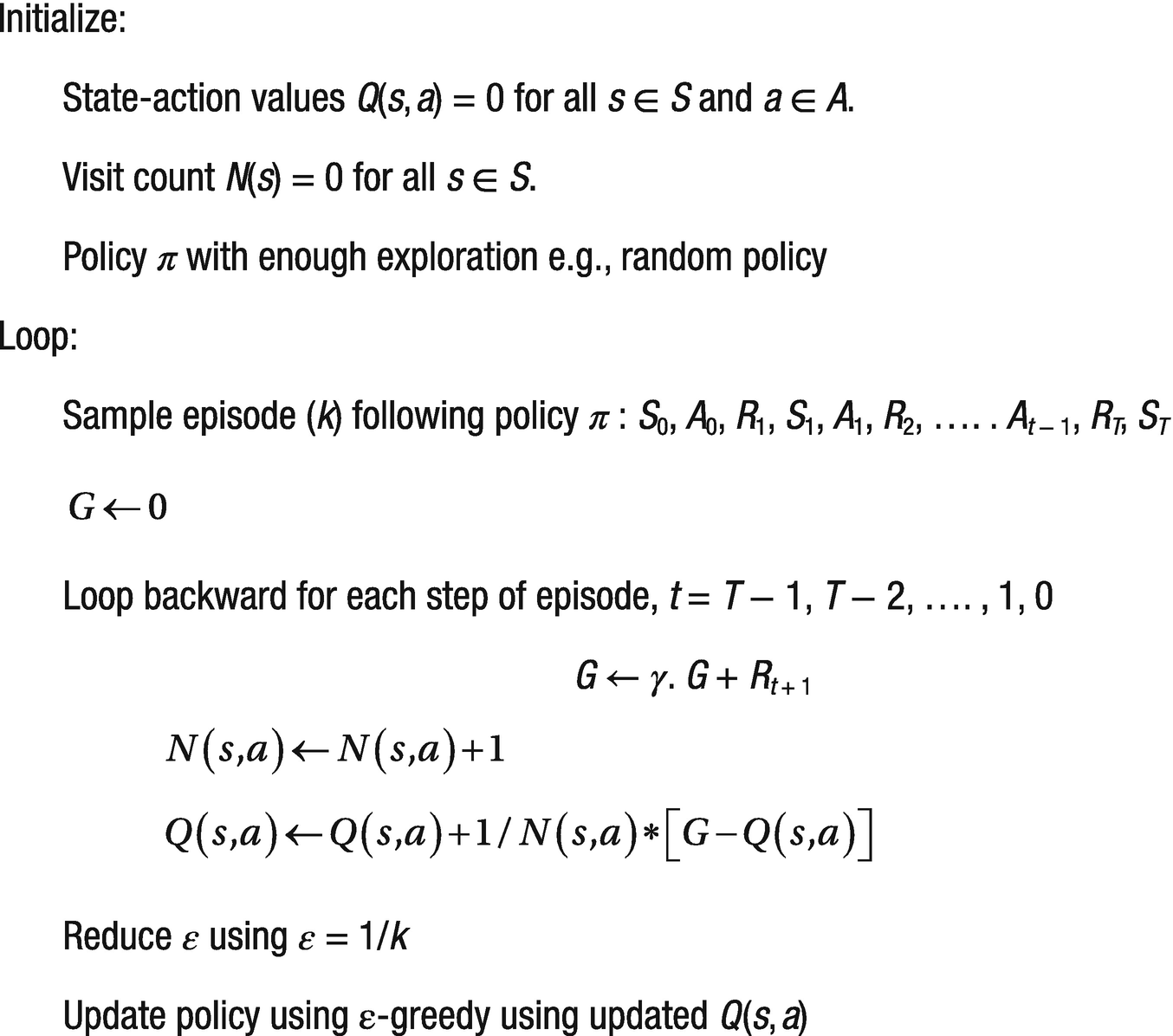
Every-visit (GLIE) MC control for policy optimization
GLIE MC Control Algorithm
So far in this chapter we have studied on-policy algorithms for prediction and control. In other words, the same policy is used to generate samples as well as policy improvement. Policy improvement is done with respect to q-values of the same ε-greedy policies. We need exploration to find Q(s, a) for all state-action pairs, which is achieved by using ε-greedy policies. However, as we progress, the ε-greedy policy with a limit is suboptimal. We need to exploit more as our understanding of the environment grows with more and more episodes. We have also seen that while theoretically the policy will converge to an optimal policy, at times it requires careful control of the ε value. The other big disadvantage of MC methods is that we need the episodes to finish before we can update q-values and carry out policy optimization. Therefore, MC methods can only be applied to environments that are episodic and where the episodes terminate. Starting in the next section, we will start looking at a different class of algorithms called temporal difference methods that combine the advantages of DP (single time-step updates) and MC (i.e., no need to know system dynamics). However, before we dive deep into TD methods, let’s go through a short section to introduce and then compare on-policy versus off-policy learning.
Off-Policy MC Control
In GLIE, we saw that to explore enough, we needed to use ε-greedy policies so that all state actions are visited often enough in limit. The policy learned at the end of the loop is used to generate the episodes for the next iteration of the loop. We are using the same policy to explore as the one that is being maximized. Such an approach is called on-policy where samples are generated from the same policy that is being optimized.
There is another approach in which the samples are generated using a policy that is more exploratory with a higher ε, while the policy being optimized is the one that may have a lower ε or could even be a fully deterministic one. Such an approach of using a different policy to learn than the one being optimized is called off-policy learning. The policy being used to generate the samples is called the behavior policy , and the one being learned (maximized) is called the target policy . Let’s look at Figure 4-7 for the pseudocode of the off-policy MC control algorithm.
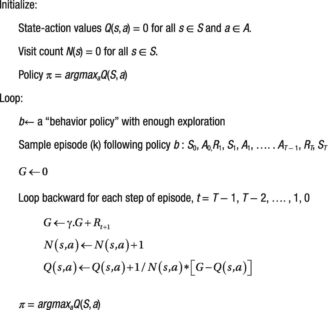
Off-policy MC control for policy optimization
Temporal Difference Learning Methods
![$$ {v}_{pi }(s)={sum}_api left(a|s
ight){sum}_{s^{prime },r}pleft({s}^{prime },r
ight|s,aleft[r+gamma {v}_{pi}left({s}^{prime}
ight)
ight] $$](https://imgdetail.ebookreading.net/202109/3/9781484268094/9781484268094__9781484268094__files__images__502835_1_En_4_Chapter__502835_1_En_4_Chapter_TeX_Equq.png)
The value of a state vπ(s) is estimated based on the current estimate of the successor states vπ(s′). This is known as bootstrapping . The estimate is based on another set of estimates. The two sums are the ones that are represented as branch-off nodes in the DP backup diagram in Figure 4-1. Compared to DP, MC is based on starting from a state and sampling the outcomes based on the current policy the agent is following. The value estimates are averages over multiple runs. In other words, the sum over model transition probabilities is replaced by averages, and hence the backup diagram for MC is a single long path from one state to the terminal state. The MC approach allowed us to build a scalable learning approach while removing the need to know the exact model dynamics. However, it created two issues: the MC approach works only for episodic environments, and the updates happen only at the end of the termination of an episode. DP had the advantage of using an estimate of the successor state to update the current state value without waiting for an episode to finish.
![$$ V(s)=V(s)+alpha left[R+gamma ast Vleft({s}^{prime}
ight)-V(s)
ight] $$](https://imgdetail.ebookreading.net/202109/3/9781484268094/9781484268094__9781484268094__files__images__502835_1_En_4_Chapter__502835_1_En_4_Chapter_TeX_Equ4.png)
The current estimate of the total return for state S = s, i.e., Gt, is now given by bootstrapping from the current estimate of the successor state (s’) shown in the sample run. In other words, Gt in equation (4.2) is replaced by R + γ ∗ V(s′), an estimate. Compared to this, in the MC method, Gt was the discounted total return for the sample run.
The TD approach described is known as TD(0), and it is a one-step estimate. The reason for calling it TD(0) will become clearer toward the end of the chapter when we talk about TD(λ). For clarity’s sake, let’s look at the pseudocode for value estimation using TD(0) given in Figure 4-8.

TD(0) policy estimation
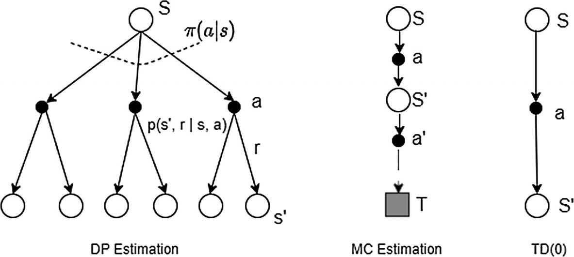
Backup diagram of DP, MC, and TD(0) compared

The difference δt is known as TD error . It represents the error (difference) in the estimate of V(s) based on reward Rt + 1 plus the discounted next time-step state value V(St + 1) and the current estimate of V(s), i.e., V(St). The value of the state is moved by a proportion (learning rate, step rate α) of this error δt.
TD has an advantage over DP as it does not require the model knowledge (transition function). A TD method has an advantage over MC as TD methods can update the state value at every step; i.e., they can be used in an online setup through which we learn as the situation unfolds without waiting for the end of episode.
Temporal Difference Control
This section will start taking you into the realm of the real algorithms used in the RL world. In the remaining sections of the chapter, we will look at various methods used in TD learning. We will start with a simple one-step on-policy learning method called SARSA. This will be followed by a powerful off-policy technique called Q-learning. We will study some foundational aspects of Q-learning in this chapter, and in the next chapter we will integrate deep learning with Q-learning, giving us a powerful approach called Deep Q Networks (DQN). Using DQN, you will be able to train game-playing agents on an Atari simulator. In this chapter, we will also cover a variant of Q-learning called expected SARSA, another off-policy learning algorithm. We will then talk about the issue of maximization bias in Q-learning, taking us to double Q-learning. All the variants of Q-learning become very powerful when combined with deep learning to represent the state space, which will form the bulk of next chapter. Toward the end of this chapter, we will cover additional concepts such as experience replay, which make off-learning algorithms efficient with respect to the number of samples needed to learn an optimal policy. We will then talk about a powerful and a bit involved approach called TD(λ) that tries to combine MC and TD methods on a continuum. Finally, we will look at an environment that has continuous state space and how we can binarize the state values and apply the previously mentioned TD methods. The exercise will demonstrate the need for the approaches that we will take up in the next chapter, covering functional approximation and deep learning for state representation. After Chapters 5 and 6 on deep learning and DQN, we will show another approach called policy optimization that revolve around directly learning the policy without needing to find the optimal state/action values.
We have been using the 4×4 grid world so far. We will now look at a few more environments that will be used in the rest of the chapter. We will write the agents in an encapsulated way so that the same agent/algorithm could be applied in various environments without any changes.
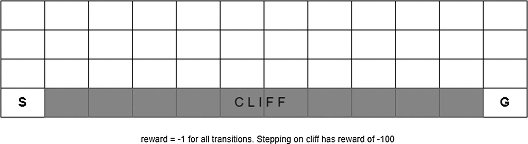
4×10 cliff world. There is a reward of -100 for stepping on the cliff and -1 for other transitions. The goal is to start from S and reach G with the best possible reward

5×5 taxi problem. There is a reward of -1 for all transitions. An episode ends when the passenger is dropped off at the destination

Cart pole problem. The objective is to balance the pole vertically for the maximum number of time steps with a reward of +1 for every time step
Having explained the various environments, let’s now jump into solving these with TD algorithms, starting first with SARSA, an on-policy method.
On-Policy SARSA
Like the MC control methods, we will again leverage GPI. We will use a TD-driven approach for the policy value estimation/prediction step and will continue to use greedy maximization for the policy improvement. Just like with MC, we need to explore enough and visit all the states an infinite number of times to find an optimal policy. Similar to the MC method, we can use a ε-greedy policy and slowly reduce the ε value to zero, i.e., for the limit bring down the exploration to zero.
![$$ Qleft({S}_t,{A}_t
ight)=Qleft({S}_t,{A}_t
ight)+alpha ast left[{R}_{t+1}+gamma ast Qleft({S}_{t+1},{A}_{t+1}
ight)-Qleft({S}_t,{A}_t
ight)
ight] $$](https://imgdetail.ebookreading.net/202109/3/9781484268094/9781484268094__9781484268094__files__images__502835_1_En_4_Chapter__502835_1_En_4_Chapter_TeX_Equ6.png)

To carry out an update as per equation (4.6), we need all the five values St, At, Rt + 1, St + 1, and At + 1. This is the reason the approach is called SARSA (state, action, reward, state, action). We will follow a ε-greedy policy to generate the samples, update the q-values using (4.6), and then based on the updated q-values create a new ε-greedy. The policy improvement theorem guarantees that the new policy will be better than the old policy unless the old policy was already optimal. Of course, for the guarantee to hold, we need to bring down the exploration probability ε to zero in the limit.
![$$ Qleft({S}_t,{A}_t
ight)=Qleft({S}_t,{A}_t
ight)+alpha ast left[{R}_{t+1}-Qleft({S}_t,{A}_t
ight)
ight] $$](https://imgdetail.ebookreading.net/202109/3/9781484268094/9781484268094__9781484268094__files__images__502835_1_En_4_Chapter__502835_1_En_4_Chapter_TeX_Equ8.png)
Let’s now look at the pseudocode of the SARSA algorithm; see Figure 4-13 .

SARSA, on-policy TD control
SARA On-Policy TD Control
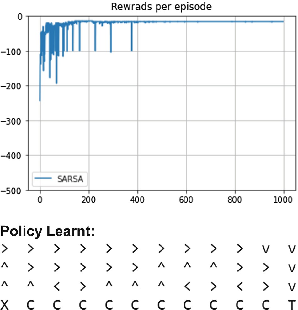
Reward graph during learning under SARSA and policy learned by agent
However, as our policy continues to explore using ε-greedy, there is always a small chance that in a state when the agent is next to a cliff cell, it takes a random action and falls off into the cliff. It demonstrates the issue of continued exploration even when enough has been learned about the environment, i.e., when the same ε-greedy policy is used for sampling as well as for improvement. We will see how this issue is avoided in Q-learning in which off-policy learning is carried out using an exploratory behavior policy to generate training samples and a deterministic policy is learned as the optimal target policy.
Next, we will study our first off-policy TD algorithm called Q-learning.
Q-Learning: An Off-Policy TD Control
In SARSA, we used the samples with the values S, A, R, S’, and A’ that were generated by the following policy. Action A’ from state S’ was produced using the ε-greedy policy, the same policy that was then improved in the “improvement” step of GPI. However, instead of generating A’ from the policy, what if we looked at all the Q(S’, A’) and chose the action A’, which maximizes the value of Q(S’,A’) across actions A’ available in state S’? We could continue to generate the samples (S, A, R, S’) (notice no A’ as the fifth value in this tuple) using an exploratory policy like ε-greedy. However, we improve the policy by choosing A’ to be argmaxA′Q(S’, A’). This small change in the approach creates a new way to learn the optimal policy called Q-learning. It is no more an on-policy learning, rather an off-policy control method where the samples (S, A, R, S’) are being generated by an exploratory policy, while we maximize Q(S’, A’) to find a deterministic optimal target policy.
We are using exploration with the ε-greedy policy to generate the samples (S, A, R, S’). At the same time, we are exploiting the existing knowledge by finding the Q maximizing action argmaxA′Q(S’, A’) in state S’. We will have lot more to say about these trade-offs between exploration and exploitation in Chapter 9.
![$$ Qleft({S}_t,{A}_t
ight)leftarrow Qleft({S}_t,{A}_t
ight)+alpha ast left[{R}_{t+1}+gamma ast {mathit{max}}_{A_{t+1}}Qleft({S}_{t+1},{A}_{t+1}
ight)-Qleft({S}_t,{A}_t
ight)
ight] $$](https://imgdetail.ebookreading.net/202109/3/9781484268094/9781484268094__9781484268094__files__images__502835_1_En_4_Chapter__502835_1_En_4_Chapter_TeX_Equ9.png)
Comparing the previous equation with equation (4.8), you will notice the subtle difference between the two approaches and how that makes Q-learning an off-policy method. The off-policy behavior of Q-learning is handy, and it makes the sample efficient. We will touch upon this in a later section when we talk about experience replay or replay buffer. Figure 4-15 gives the pseudocode of Q-learning.

Q-learning, off-policy TD control
Q Learning Off-Policy TD Control
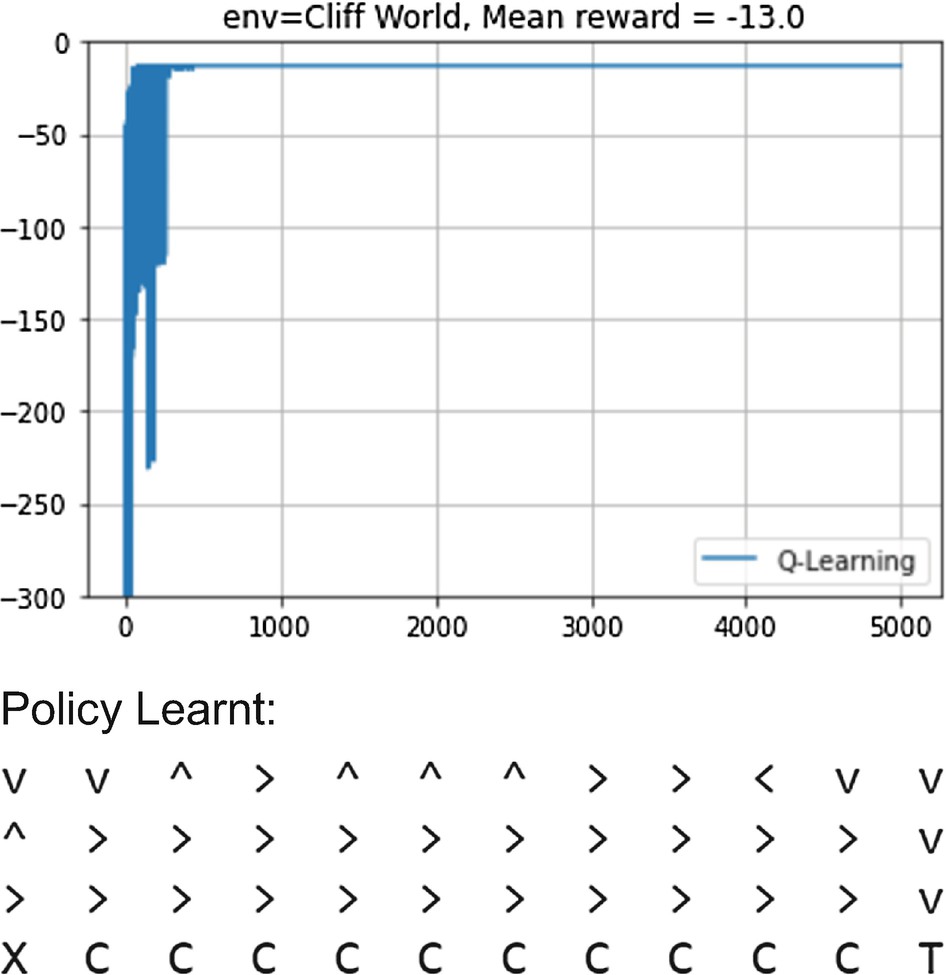
Reward graph during learning under Q-learning and policy learned by agent
The file listing4_4.ipynb also shows the learning curve when the Q-agent is applied to the taxi world environment. We will be revisiting Q-learning in next chapter on the deep learning approach to the state value approximation. Under that setup, Q-learning is called DQN. DQN with its variants will be used to train a game-playing agent on some Atari games.
To conclude the discussion on Q-learning, let’s look at a particular issue that Q-learning may introduce, that of maximization bias.
Maximization Bias and Double Learning
If you look back at equation (4.10), you will notice that we are maximizing over A’ to get the max value Q(S’, A’). Similarly, in SARSA, we find a new ε-greedy policy that is also maximizing over Q to get the action with highest q-value. Further, these q-values are estimates themselves of the true state-action values. In summary, we are using a max over the q-estimate as an “estimate” of the maximum value. Such an approach of “max of estimate” as an “estimate of max” introduces a +ve bias.
To see this, consider a scenario where the reward in some transition takes three values: 5, 0, +5 with an equal probability of 1/3 for each value. The expected reward is zero, but the moment we see a +5, we take that as part of the maximization, and then it never comes down. So, +5 becomes an estimate of the true reward that otherwise in expectation is 0. This is a positive bias introduced due to maximization step.
One of the ways to remove the +ve bias is to use a set of two q-values. One q-value is used to find the action that maximizes the q-value, and the other set of q-values is then used to find the q-value for that max action. Mathematically, it can be represented as follows:
Replace maxAQ(S, A) with Q1(S, argmaxAQ2(S, A)).
We are using Q2 to find the maximizing action A, and then Q1 is used to find the maximum q-value. It can be shown that such an approach removes the +ve or maximization bias. We will revisit this concept when we talk about DQN.
Expected SARSA Control
![$$ Qleft({S}_t,{A}_t
ight)leftarrow Qleft({S}_t,{A}_t
ight)+alpha ast left[{R}_{t+1}+gamma ast {sum}_api left(a|{S}_{t+1}
ight).Qleft({S}_{t+1},a
ight)-Qleft({S}_t,{A}_t
ight)
ight] $$](https://imgdetail.ebookreading.net/202109/3/9781484268094/9781484268094__9781484268094__files__images__502835_1_En_4_Chapter__502835_1_En_4_Chapter_TeX_Equ10.png)
Expected SARSA has a lower variance as compared to the variance seen in SARSA due to the random selection of At + 1. In expected SARSA, instead of sampling, we take the expectation over all possible actions.
In the cliff world problem, we have deterministic actions, and hence we can set the learning rate α = 1 without any major impact on the learning quality. We give the pseudocode for the algorithm. It mirrors Q-learning except for the update logic of taking expectation instead of maximization. We can run expected SARSA as on-policy, which is what we will do while testing it against the cliff and taxi worlds. It can also be run off-policy where the behavior policy is more exploratory and the target policy π follows a deterministic greedy policy. See Figure 4-17.

Expected SARA TD control
Expected SARSA TD Control

Reward graph with expected SARSA in the cliff world and policy learned by the agent
Replay Buffer and Off-Policy Learning
Off-policy learning involves two separate policies: behavior policy b(a| s) to explore and generate examples; and π(a| s), the target policy that the agent is trying to learn as the optimal policy. Accordingly, we could use the samples generated by the behavior policy again and again to train the agent. The approach makes the process sample efficient as a single transition observed by the agent can be used multiple times.
This is called experience replay . The agent is collecting experiences from the environment and replaying those experiences multiple times as part of the learning process. In experience replay, we store the samples (s, a, r, s', done) in a buffer. The samples are generated using an exploratory behavior policy while we improve a deterministic target policy using q-values. Therefore, we can always use older samples from a behavior policy and apply them again and again. We keep the buffer size fixed to some predetermined size and keep deleting the older samples as we collect new ones. The process makes learning sample efficient by reusing a sample multiple time. The rest of the approach remains the same as an off-policy agent.
Q-Learning with Replay Buffer
The Q-agent with the replay buffer is supposed to improve the initial convergence by sampling repeatedly from the buffer. The sample efficiency will become more apparent when we look at DQN. Over the long run, there won’t be any significant difference between the optimal values learned with or without the replay buffer. It has another advantage of breaking the correlation between samples. This aspect will also become apparent when we look at deep learning with Q-learning, i.e., DQN.
Q-Learning for Continuous State Spaces
Until now all the examples we have looked at had discrete state spaces. All the methods studied so far could be categorized as tabular methods. The state action space was represented as a matrix with states along one dimension and actions along the cross-axis.
We will soon transition to continuous state spaces and make heavy use of deep learning to represent the state through a neural net. However, we can still solve many of the continuous state problems with some simple approaches. In preparation for the next chapter, let’s look at the simplest approach of converting continuous values into discrete bins. The approach we will take is to round off continuous floating-point numbers with some precision, e.g., for a continuous state space value between -1 to 1 being converted into -1, -0.9, -0.8, … 0, 0.1, 0.2, … 1.0.
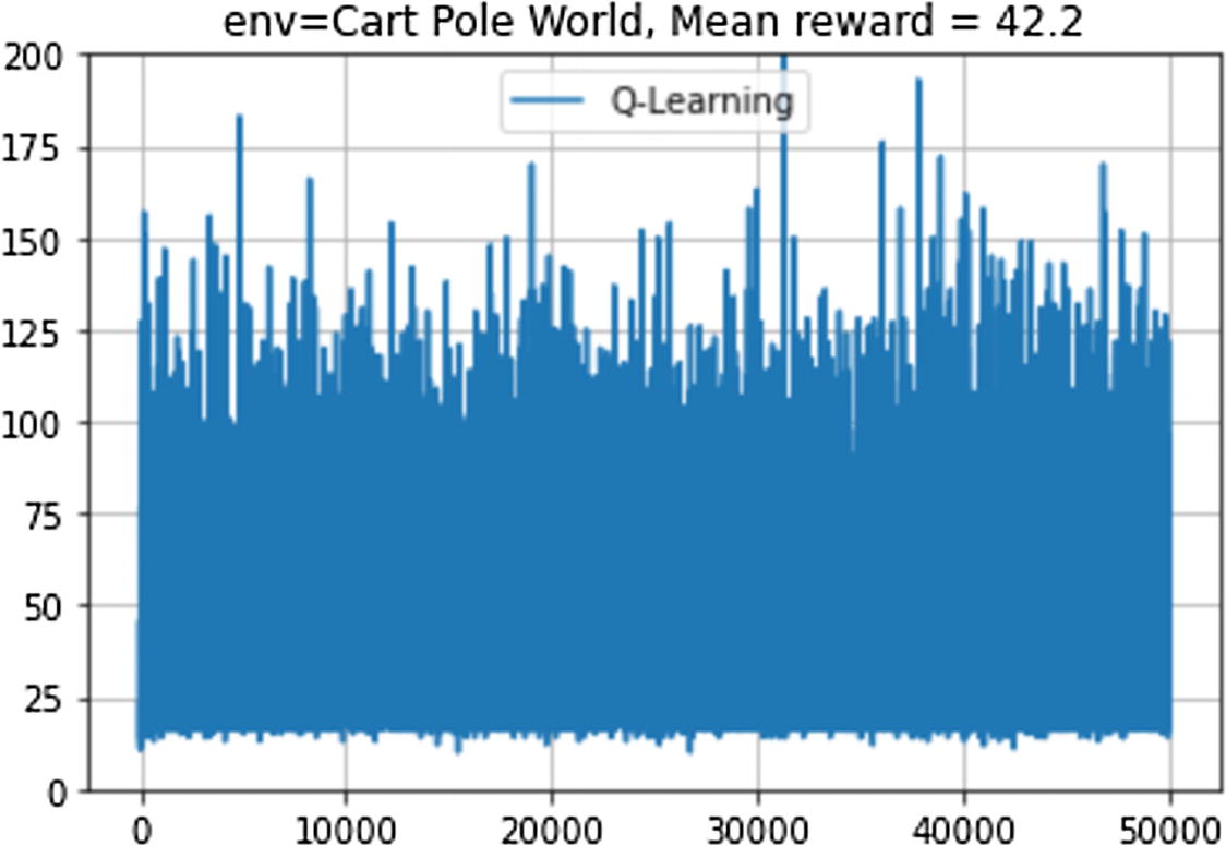
Reward graph with Q-learning on CartPole continuous state space environment
Q-Learning (Off-Policy) on Continuous State Environment
The Q-agent with discrete discretization of states is able to get about 50 rewards compared to the maximum reward of 200. In subsequent chapters, we will study other more powerful methods to obtain more rewards.
n-Step Returns
In this section, we will unify the MC and TD approaches. MC methods sample the return from a state until the end of the episode, and they do not bootstrap. Accordingly, MC methods cannot be applied for continuing tasks. TD, on the other hand, uses one-step return to estimate the value of the remaining rewards. TD methods take a short view of the trajectory and bootstrap right after one step.

Backup diagrams of n-step methods with TD(0) and MC at two extremes, n=1 and n=∞ (end of episode)
The approach of n-step can be used in an on-policy setting. We can have n-step SARSA and n-step expected SARSA, and these are natural extensions of what we have learned so far. However, using an n-step approach in off-policy learning would require us to factor one more concept, the relative difference of observing a specific n-step transition across states under behavior policy versus that under target-policy. To use the data from behavior policy b(a| s) for optimizing target policy π(a| s), we need to multiply the n-step returns observed under the behavior policy with a ratio called importance sampling ratio .


The importance sampling ratio ensures that the return of a trajectory observed under the behavior policy is adjusted up or down based on the relative chance of observing a trajectory under the target policy versus the chance of observing the same trajectory under the behavior policy.
Nothing comes for free, which is the case with importance sampling. The importance sampling ratio can cause wide variance. Plus, these are not computationally efficient. There are many advanced techniques like discount-aware importance sampling and per-decision importance sampling , which look at the importance sampling and rewards in various different ways to reduce the variance and also to make these algorithms efficient.
We will not be going into the details of implementing these algorithms in this book. Our key focus was to introduce these at a conceptual level and make you aware of the advanced techniques.
Eligibility Traces and TD(λ)
Eligibility traces unify the MC and TD methods in an algorithmically efficient way. TD methods when combined with eligibility trace produce TD(λ) where λ = 0, making it equivalent to the one-step TD that we have studied so far. That’s the reason why one-step TD is also known as TD(0). The value of λ = 1 makes it similar to the regular ∞-step TD or in other words an MC method. Eligibility trace makes it possible to apply MC methods on nonepisodic tasks. We will cover only high-level concepts of eligibility trace and TD(λ).
In the previous section, we looked at n-step returns with n=1 taking us to the regular TD method and n=∞ taking us to MC. We also touched upon the fact that neither extreme is good. An algorithm performs best with some intermediate value of n. n-step offered a view on how to unify TD and MC. What eligibility does is to offer an efficient way to combine them without keeping track of the n-step transitions at each step. Until now we have looked at an approach of updating a state value based on the next n transitions in the future. This is called the forward view. However, you could also look backward, i.e., at each time step t, and see the impact that the reward at time step t would have on the preceding n states in past. This is known as backward view and forms the core of TD(λ). The approach allows an efficient implementation of integrating n-step returns in TD learning.


The previous expression is similar to the target value for state-action updates of TD(0) in (4.7).


The TD(λ) algorithm uses the previous λ-return with a trace vector known as eligibility trace to have an efficient online TD method using the “backward” view. Eligibility trace keeps a record of how far in the past a state was observed and by how much would that state’s estimate would be impacted by the current return observed.
We will stop here with the basic introduction of λ-returns, eligibility trace, and TD(λ). For a detailed review of the mathematical derivations as well as the various algorithms based on them, refer to the book Reinforcement Learning: An Introduction by Barto and Sutton, 2nd edition.
Relationships Between DP, MC, and TD
At the beginning of the chapter, we talked about how the DP, MC, and TD methods compare. We introduced the MC methods followed by the TD methods, and then we used n-step and TD(λ) to combine MC and TD as two extremes of the sample-based model-free learning.
Comparison of DP and TD Methods in the Context of Bellman Equations
Full Backup (DP) | Sample Backup (TD) | |
|---|---|---|
Bellman expectation equation for vπ(s) | Iterative policy evaluation | TD prediction |
Bellman expectation equation for qπ(s, a) | Q-policy iteration | SARSA |
Bellman optimality equation for qπ(s, a) | Q-value iteration | Q-learning |
Summary
In this chapter, we looked at the model-free approach to reinforcement learning. We started by estimating the state value using the Monte Carlo approach. We looked at the “first visit” and “every visit” approaches. We then looked at the bias and variance trade-off in general and specifically in the context of the MC approaches. With the foundation of MC estimation in place, we looked at MC control methods connecting it with the GPI framework for policy improvement that was introduced in Chapter 3. We saw how GPI could be applied by swapping the estimation step of the approach from DP-based to an MC-based approach. We looked in detail at the exploration exploitation dilemma that needs to be balanced, especially in the model-free world where the transition probabilities are not known. We then briefly talked about the off-policy approach in the context of the MC methods.
TD was the next approach we looked into with respect to model-free learning. We started off by establishing the basics of TD learning, starting with TD-based value estimation. This was followed by a deep dive into SARSA, an on-policy TD control method. We then looked into Q-learning, a powerful off-policy TD learning approach, and some of its variants like expected SARSA.
In the context of TD learning, we also introduced the concept of state approximation to convert continuous state spaces into approximate discrete state values. The concept of state approximation will form the bulk of the next chapter and will allow us to combine deep learning with reinforcement learning.
Before concluding the chapter, we finally looked at n-step returns, eligibility traces, and TD(λ) as ways to combine TD and MC into a single framework.