In this chapter, we will do a deep dive into Q-learning combined with function approximation using neural networks. Q-learning in the context of deep learning using neural networks is also known as Deep Q Networks (DQN). We will first summarize what we have talked about so far with respect to Q-learning. We will then look at code implementations of DQN on simple problems followed by training an agent to play Atari games. Following this, we will extend our knowledge by looking at various modifications that can be done to DQN to improve the learning, including some very recent and state-of-the-art approaches. Some of these approaches may involve a bit of math to understand the rationale for these approaches. However, we will try to keep the math to a minimum and include just the required details to appreciate the background and reasoning. All the examples in this chapter will be coded using either the PyTorch or TensorFlow library. Some code walk-throughs will have the code for both PyTorch and TensorFlow, while others will be discussed using only PyTorch.
Deep Q Networks
In Chapter 4 we talked about Q-learning as a model-free off-policy TD control method. We first looked at the online version where we used an exploratory behavior policy (ε-greedy) to take a step (action A) while in state S. The reward R and next state S’ were then used to update the q-value Q(S, A). Figure 4-14 and Listing 4-4 detailed the pseudocode and actual implementation. The update equation used in this context is given here. You may want to revisit this before you move forward.
(6.1)
We briefly talked about maximization bias and the approach of double Q-learning wherein we use two tables of q-values. We will have more to say about it in this chapter when we look at double DQN.
Following this, we looked at the approach of using a sample multiple times to convert online TD updates to batch TD updates, making it more sample efficient. It introduced us to the concept of a replay buffer. While it was only about sample efficiency in the context of discrete state and state-action spaces, with function approximation with neural networks, it becomes pretty much a must-have to make deep learning neural networks converge. We will revisit this again, and when we talk about prioritized replay, we will look at other options to sample transitions/experiences from the buffer.
Moving along, in Chapter 5, we looked at various approaches of function approximation. We looked at tile encoding as a way to achieve linear function approximation. We then talked about DQN, i.e., batch Q-learning with neural networks as function approximators. We went through a long derivation to arrive at a weight (with neural network parameters) update equation as given in equation (5.25). This is reproduced here:
(6.2)
Please also note that we are using subscript i to denote the sample in the mini-batch and i to denote the index at which the weights are updated. Equation (6.2) is the one we will be using extensively in this chapter. We will make various adjustments to this equation as we talk about different modifications and study their impact.
We also talked about not having a theoretical guarantee of convergence under nonlinear function approximation with a gradient update. We will have more to say about that in this chapter. The Q-learning approach was for discrete states and actions where the update to the q-value was using (6.1) as compared to adjusting the weight parameters for the deep learning–based approach in DQN. The Q-learning case had guarantees of convergence, while with DQN we had no such guarantee. DQN is computationally intensive as well. However, despite these shortcomings in DQN, DQN makes it possible to train agents using raw images, something not at all conceivable in the case of plain Q-learning. Let’s now put equation (6.2) to practice to train the DQN agents in various environments.
Let’s revisit the CartPole problem, which has a four-dimensional continuous state with values for the current cart position, velocity, angle of the pole, and angular velocity of the pole. The actions are of two types: push the cart to the left or push the cart to the right with the aim of keeping the pole balanced for as long as possible. The following are the details of the environment:
Observation:
Type: Box(4)
Num Observation Min Max
0 Cart Position -4.8 4.8
1 Cart Velocity -Inf Inf
2 Pole Angle 0.418 rad (-24 deg) 0.418 rad (24 deg)
3 Pole Angular Velocity -Inf Inf
Actions:
Type: Discrete(2)
Num Action
0 Push cart to the left
1 Push cart to the right
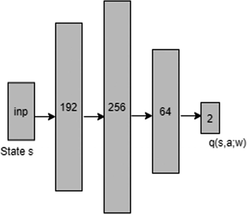
We will build a small neural network with 4 as the input dimension, three hidden layers, followed by an output layer of dimension 2 being the number of possible actions. Figure 6-1 shows the network diagram.
Figure 6-1
Simple neural network
We will use PyTorch’s nn.Module class to build the network. We will also implement some additional functions. Function get_qvalues takes a batch of states as input, i.e., a tensor of dimension (N×4) where N is the number of samples. It passes the state values through the network to produce the q-values. The output vector has size (N×2); i.e., one row for each input. Each row has two q-values, one for the left-push action and another for the right-push action. Function sample_actions in the same class takes in a batch of q-values (N×2). It uses the ε-greedy policy (equation 4.3) to choose an action. The output is the (N×1) vector. Listing 6-2 shows the code for this in PyTorch. Listing 6-3 shows the same code in TensorFlow 2.0’s eager execution mode. You can find the complete PyTorch implementation in file listing6_1_dqn_pytorch.ipynb and for TensorFlow in file listing6_1_dqn_tensorflow.ipynb.
Note While not essential, you will gain more from the code discussions with some prior knowledge of PyTorch or TensorFlow. You should be able to create basic networks, define loss functions, and carry out basic training steps for optimization. TensorFlow’s new eager execution model is similar to PyTorch. For this reason, we will provide the code in both libraries for a limited set of examples to get you started. Otherwise, most of the code in the book will be in PyTorch.
Listing 6-2 shows the same code in TensorFlow 2.x using the Keras interface. We are using the new eager execution model, which is similar to the approach that PyTorch takes. TensorFlow used to have a different model in earlier versions, which was a little bit hard to conceptualize with two separate phases: one of symbolic graphs to build all the network operations and then a second phase of training of the model by passing data as tensors into the model build in the first phase.
The code for the replay buffer is simple. We have a buffer called self.buffer to hold the previous examples. Function add takes in (state, action, reward, next_state, done), the values from a single step/transition by the agent, and adds that to the buffer. If the buffer has already reached full length, it discards the oldest transition to make space for the new addition. Function sample takes an integer batch_size and returns batch_size samples/transitions from the buffer. In this vanilla implementation, each transition stored in the buffer has equal probability of getting sampled. Listing 6-3 shows the code for the replay buffer.
Moving ahead, we have a utility function, play_and_store, that takes in an env (e.g., CartPole), an agent (e.g., DQNAgent), an exp_replay (ReplayBuffer), the agent’s start_state, and n_steps (i.e., number of steps/actions to take in the environment). The function makes the agent take n_steps number of steps starting from the initial state start_state. The steps are taken based on the current ε-greedy policy that the agent is following using agent.sample_actions and records these n_steps transitions in the buffer. Listing 6-4 shows the code.
# Play the game for n_steps and record transitions in buffer
for _ in range(n_steps):
qvalues = agent.get_qvalues([s])
a = agent.sample_actions(qvalues)[0]
next_s, r, done, _ = env.step(a)
sum_rewards += r
exp_replay.add(s, a, r, next_s, done)
if done:
s = env.reset()
else:
s = next_s
return sum_rewards, s
Listing 6-4
Implementation of Function play_and_record
Next, we look at the learning process. We first build the loss, L, that we want to minimize. It is the averaged squared error between the target value of the current state action using a one-step TD value and the current state value. As discussed in Chapter 5, we use a copy of the original neural network that has weights w− (w with superscript −). We use the loss to calculate the gradient of the agent (online/original) network’s weight w and take a step in the negative direction of the gradient to reduce the loss. Please note that as discussed in Chapter 5, we keep the target network with weights w− frozen and update these weights on a less frequent basis. To quote from the section on batch methods of DQN in Chapter 5:
Here we have used a different weight vector wt−to calculate the estimate of target. Essentially, we have two networks, one called online with weights “w"which is being updated as per equation (5.24) and second a similar network called target network but with a copy of the weight “w” called “w−". Weight vector “w−is updated less frequently say after every 100 updates of online network. This approach keeps the target network constant and allows us to use the machinery of supervised learning.
The loss function is as follows:
(6.3)
We take a gradient (derivative) of L with regard to w and then use this gradient to update the weights w of the online network. The equations are as follows:
(6.4)
(6.5)
Combining the two, we get our familiar update in equation (6.2). However, in PyTorch and TensorFlow, we do not carry out the updates by directly coding them as it is not easy to calculate the gradients . That’s one of the primary reasons to use packages like PyTorch and TensorFlow, which automatically calculate gradients based on the operations performed to calculate the loss metric L. We just need a function to calculate that metric L. This is done by the function compute_td_loss. It takes in a batch of (states, actions, rewards, next_states, done_flags). It also takes in the discount parameter γ as well as the agent/online and target networks. The function then computes loss L as per equation (6.3). Listing 6-5 gives the implementation in PyTorch, and Listing 6-6 gives it in TensorFlow.
loss = tf.keras.losses.MSE(target_qvalues_for_actions, predicted_qvalues_for_actions)
return loss
Listing 6-6
Compute TD Loss in TensorFlow
At this point, we have all the machinery to train the agent to balance the pole. First, we define some hyperparameters like batch_size, total training steps total_steps, and the rate at which exploration ε will decay. It starts at 1.0 and slowly reduces the exploration to 0.05 as the agent learns the optimal policy. We also define an optimizer, which can take in the loss L as created in the previous listing and helps us take a gradient step to adjust the weights, essentially implementing equations (6.4) and (6.5). Listing 6-7 gives the training code in PyTorch. Listing 6-8 gives the same code in TensorFlow.
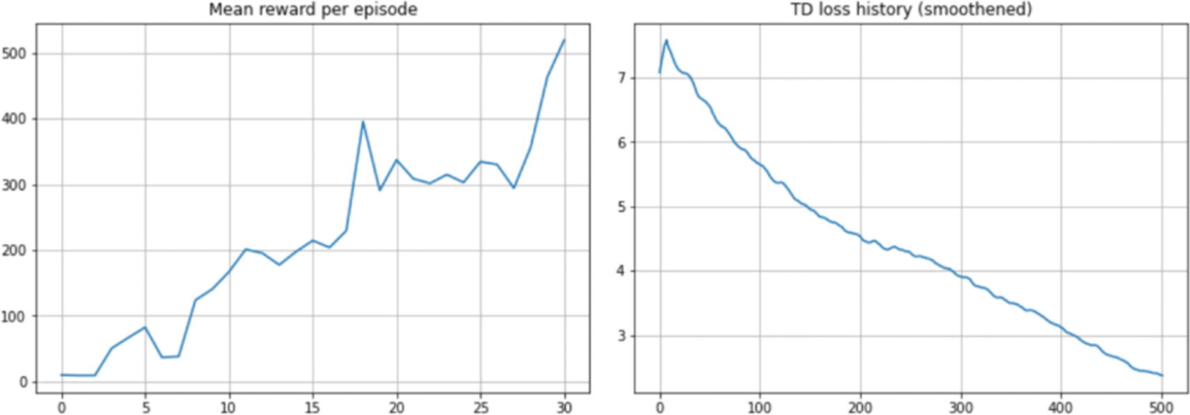
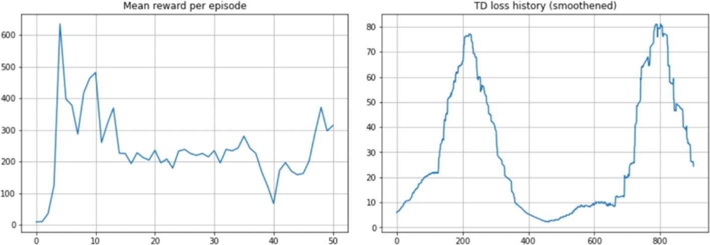
We now have a fully trained agent. We train the agent and plot the mean reward per episode periodically as we train the agent for 50,000 steps. In the left plot in Figure 6-2, the x-axis value of 10 corresponds to the 10,000th step. We also plot the TD loss every 20 steps, and that’s why we have the x-axis on the right plot going from 0 to 2500, i.e., 0 to 2500x20=50,000 steps. Unlike supervised learning, the targets are not fixed. We keep the target network fixed for a short duration and update it periodically by refreshing the target network weights with the online network. Also, as discussed, nonlinear function approximation (neural networks) with off-policy learning (Q-learning) and bootstrapped targets (the target network being just an estimate of the actual value and the estimate formed using the current estimates of other q-values) has no convergence guarantee. The training may see losses going up and exploding or fluctuating. This loss graph is counterintuitive as compared to the loss graphs in the usual supervised learning. Figure 6-2 shows the graphs from the training DQN.
Figure 6-2
Training curves for DQN
The code notebooks listing6_1_dqn_pytorch.ipynb and listing6_1_dqn_tensorflow.ipynb have some more code to record the behavior of how the trained agent performs as a video file and then play the video to show the behavior.
This completes the implementation of a full DQN using deep learning to train an agent. It might look like overkill to use a complex neural network for such a simple network. The core idea was to focus on the algorithm and teach you how to write a DQN learning agent. We will now use the same implementation with minor tweaks so that the agent can play Atari games using the game image pixel values as the state.
Atari Game-Playing Agent Using DQN
In a 2013 seminal paper titled “Playing Atari with Deep Reinforcement Learning,”1 the authors used a deep learning model to create a neural network–based Q-learning algorithm. They christened it Deep Q Networks. This is exactly what we implemented in the previous section. We will now briefly discuss the additional steps the authors took to train the agent to play Atari games. The main gist is the same as the previous section with two key differences: using game image pixel values as state inputs that require some preprocessing, and using convolutional networks inside an agent instead of linear layers that we saw in the previous section. The rest of the approach to calculate the loss L and carry out the training remains the same as the previous section. Please note that training with convolution networks takes a lot of time, especially on regular PCs/laptops. Get ready to watch the training code run for hours even on moderately powerful GPU-based machines.
You can find the complete code to train the agent in PyTorch in file listing6_2_dqn_atari_pytorch.ipynb. You can find the same code in TensorFlow in listing6_2_dqn_atari_tensorflow.ipynb. The Gym library has implemented many of the transformations needed on an Atari image, and wherever possible, we will be using the same thing.
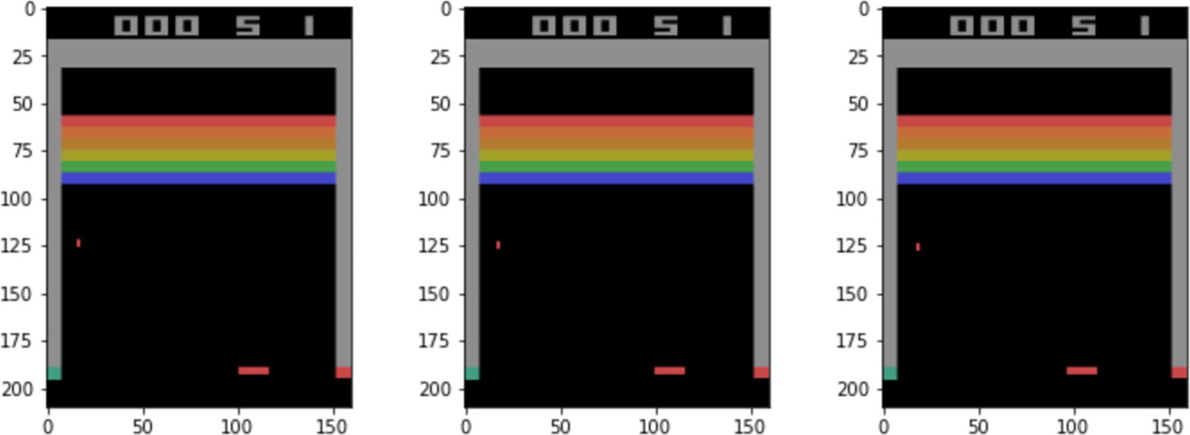
Let’s now talking about the image preprocessing done to get the image pixel values ready for feeding into the deep learning network. We will talk about this in the context of a game called Breakout in which there is a paddle at the bottom, and the idea is to move the paddle to ensure the ball does not fall below it. We need to use the paddle to hit and take out as many bricks as possible. Each time the ball misses the paddle, the player loses a life. The player has five lives to start. Figure 6-3 shows three frames of the game.
Figure 6-3
Atari Breakout game images
Atari game images are 210×160-pixel images with a 128-color palette. We will do preprocessing to prune down the image and make the convolutional network run faster. We scale down the images. We also remove some of the information from the sides, keeping just the relevant part of the images for training. We can convert the image to grayscale again to reduce the size of the input vector, with one channel of grayscale instead of three channel of colors for RGB (the Red, Green, Blue channels). A preprocessed single frame of the image of size (1×84×84 in PyTorch or 84×84×1 in TensorFlow) just gives the static state. The position of the ball or paddle does not tell us the direction in which both are moving. Accordingly, we will stack a few consecutive frames of the game images together to train the agent. We will stack four reduced-size grayscale images that will the state s feeding into the neural network. The input (i.e. state s) will be of size 4×84×84 in PyTorch and 84×84×4 in TensorFlow, where 4 refers to the four frames of the game images and 84×84 is the grayscale image size of each frame. Stacking four frames together will allow the agent network to infer the direction of movement of the ball and paddle. We use Gym’s AtariPreprocessing to carry out image reduction from a 210×160×3 size array of color images to an 84×84 array of grayscale images. This function also scales down individual pixel values from the range (0,255) to (0.0, 1.0) by setting scale_obs=True. Next we use FrameStack to stack together four images as discussed earlier. Finally, in line with the original approach, we also clip the reward values to just -1 or 1. Listing 6-9 gives the code carrying out all these transformations.
The previous preprocessing step produces the final state that we will be feeding into the network. This will be of size 4×84×84 in PyTorch and 84×84×4 in TensorFlow, where 4 refers to the four frames of the game images and 84×84 is the grayscale image size of each frame. Figure 6-4 shows the input to the network.
Figure 6-4
Processed image to be used as state input into the neural network
Next, we build the neural network that will take in the previous image, i.e., the state/observation s, and produce q-values for all four actions in this case. The actions for this game are ['NOOP', 'FIRE', 'RIGHT', 'LEFT'], using the spacebar to start, i.e., fire, pressing A on the keyboard to move the paddle left, pressing D to move the paddle right, and finally pressing Esc to quit the game. The following is the specification of the network we will build:
input: tensorflow: [batch_size, 84, 84, 4]
pytorch: [batch_size, 4, 84, 84]
1st hidden layer: 16 nos of 8x8 filters with stride 4 and ReLU activation
2nd hidden layer: 32 nos of 4x4 filters with stride of 2 and ReLU activation
3nd hidden layer: Linear layer with 256 outputs and ReLU activation
output layer: Linear with “n_actions” units with no activation
The rest of the code is similar to what we had earlier. Listing 6-10 and Listing 6-11 show the code of the modified DQN agents in PyTorch and TensorFlow, respectively.
You will notice the similarity in the code between PyTorch and TensorFlow in eager execution mode. You are well advised to focus on one framework and master the concepts. Once you have mastered one, it will be easy to port the code to the other framework. We will be using PyTorch in this book for the majority of the examples, with some TensorFlow versions here and there.
Except for these two changes, i.e., some problem-specific preprocessing and a problem-appropriate neural network, the rest of the code remains the same between CartPole and Atari. You can also use the Atari version to train the agent on any version of the Atari game. Further, except for these two changes, the same code can be used to train the DQN agent for any environment. You can look into the available Gym environments from the Gym library documentation and try to modify the code from listing6_1_dqn_pytorch.ipynb or listing6_1_dqn_atari_pytorch.ipynb to train the agents for different environments.
This completes the implementation and training of DQN. Now that we know how to train a DQN agent, we will look into some issues and various approaches we could take to modify the DQN. As we talked about at the beginning of the chapter, we will look at some recent and state-of-the-art variations.
Prioritized Replay
In the previous chapter, we saw how to use a batch version of updates in DQN that addresses some key issues that are there in the online version, with updates being done with each transition and a transition being discarded right after that one step of learning. The following are the key issues in the online versions:
The training samples (transitions) are correlated, breaking i.i.d. (independent identically distributed) assumptions. With online learning, we have transitions coming in a sequence that are correlated. Each transition is linked to the previous one. This breaks the i.i.d. assumption that is required to apply gradient descent.
As the agent learns and discards, it may never get to visit the initial exploratory transitions. If the agent goes down a wrong path, it will keep seeing examples from that part of the state space. It may settle on a very suboptimal solution.
With neural networks, learning on a single transition basis is hard and inefficient. There will be too much variance for the neural networks to learn anything effective. Neural networks work best when they learn in batches of training samples.
These were addressed in DQN by using an experience replay where all transitions are stored. Each transition is a tuple of (state, action, reward, next_state, done). As the buffer gets full, we discard old samples to add new ones. We then sample a batch from the current buffer with each transition in the buffer having equal probability of being selected in a batch. It allows rare and more exploratory transitions to be picked multiple times from the buffer. However, a plain-vanilla experience replay does not have any way to choose the important transitions with some priority. Would it help to somehow assign an importance score to each transition stored in the replay buffer and sample the batch from the buffer using these importance scores as the probability of selection, assigning a higher probability of selection to important transitions as signified by their respective importance score?
This is what the authors of the paper “Prioritized Experience Replay”2 from DeepMind explored in 2016. We will follow the main concepts of this paper to create our own implementation of experience replay and apply it on the DQN agent for the CartPole environment. Let’s start by talking a little bit about how these importance scores are assigned and how the loss L is modified.
The key approach of this paper is to assign importance scores to training samples in the buffer using their TD errors. When a batch of samples is picked from the buffer, we calculate the TD error as part of the loss L calculation. The TD error is given by this equation:
(6.6)
It appears inside equation (6.3) where we calculate the loss. The error is squared and averaged over all samples to calculate the magnitude of updates to weight vectors as shown in equations (6.4) and (6.5). The magnitude of TD error δi denotes the contribution that the sample transition (i) would have on the update. The authors used this reasoning to assign an importance score pi to each sample, where pi is given by this equation:
(6.7)
A small constant ε is added to avoid the edge case of pi being zero when TD error δi is zero. When a new transition is added to the buffer, we assign it the max of pi across all current transitions in the buffer. When a batch is picked for training, we calculate the TD error δi of each sample as part of the loss/gradient calculation. This TD error is then used to update the importance score of these samples back in the buffer.
There is another approach of rank-based prioritization that the paper talks about. Using that approach, , where rank(i) is the rank of transition(i) when the replay buffer transitions are sorted based on |δi|. In our code example, we will be using the first approach, which is called proportional prioritization.
Next, at the time of sampling, we convert pi to probabilities by using the following equation:
(6.8)
Here, P(i) denotes the probability of transition (i) in the buffer getting sampled and as part of the training batch. This assigns a higher sampling probability to the transitions that have a higher TD error. Here, α is a hyperparameter, which was tuned using grid search, and the authors found α = 0.6 to be the best for the proportional variant that we will be implementing.
The previous approach of breaking the uniform sampling with some kind of sampling based on importance introduces bias. We need to correct the bias while calculating the loss L. In the paper, this was corrected using importance sampling by weighing each sample with weight wi and then summing it up to get the revised loss function L. The equation for calculating weights is as follows:
(6.9)
Here, N is the number of samples in the training batch, and P(i) is the probability of selecting a sample as calculated in the previous expression earlier. β is another hyperparameter for which we will use a value of 0.4 from the paper. The weights are further normalized by to ensure that the weights stay within bounds.
(6.10)
With these changes in place, the loss L equation is also updated to weigh each transition in the batch with wi as follows:
(6.11)
Notice the wi in the equation. After L is calculated, we follow the usual gradient step using back propagation of the loss gradient with respect to the online neural network weights w.
Remember, the TD error in the previous equation is used to update the importance score back in the replay buffer for these transitions in the current training batch. This completes the theoretical discussion on the prioritized replay. We will now look at the implementation. The complete code of training a DQN agent with prioritized replay is given in listing6_3_dqn_prioritized_replay.ipynb, which has two flavors, one in PyTorch and another in TensorFlow. However, from this point on, we will only list the PyTorch versions. You are advised to study the code in detail along with the referenced paper after going through the explanations given next. The ability to follow the academic papers and match the details in the paper to working code is an important part of becoming a good practitioner. The explanation is to just get you started. For a firm grasp of the material, you should follow the accompanying code in detail. It will be even better if you try to code it yourself after absorbing how the code works.
Getting back to the explanation, we first look at the prioritized replay implementation, which is the major change in the code from the previous DQN training notebook. Listing 6-12 gives the code for prioritized replay. Most of the code is similar to that of the plain ReplayBuffer we saw earlier. We now have an additional array called self.priorities to hold the importance/priority score pi for each sample. Function add is modified to assign pi to the new sample being added. It is just the max of values in the array self.priorities. Function sample is the one where there is maximum change. The first probabilities are calculated using equation (6.8), and then the weights are calculated using (6.9) and (6.10). The function now returns additional two arrays: the array of weights np.array(weights) and the array of index np.array(idxs). The array of indexes contains the indexes of the samples in the buffer that were sampled in the batch. This is required so that after the calculation of TD error in the loss step, we can update the priority/importance back in the buffer. Function update_priorities(idxs, new_priorities) is exactly for that purpose.
Next, we look at the loss calculation. The code is almost similar to the TD loss computation we saw in Listing 6-5. There are two changes. The first is multiplying the TD error with weights, in line with equation (6.11). The second change is calling update_priorities from inside the function to update the priorities back in the buffer. Listing 6-13 shows the code for the revised TD_loss compute_td_loss_priority_replay computation.
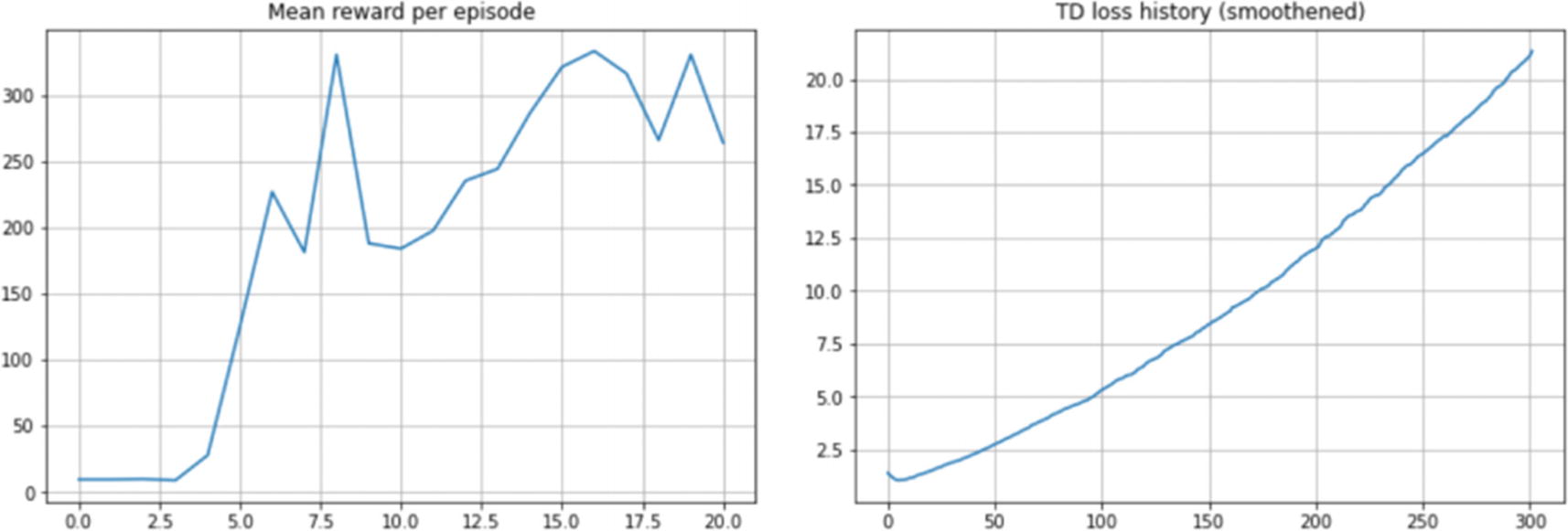
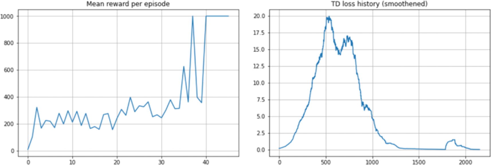
The training code remains the same as before. You can look at the listing6_3_dqn_prioritized_replay_pytorch.ipynb notebook to see the details. Like before, we train the agent, and we can see that the agent learns to balance the pole really well with this approach. Figure 6-5 shows the training curves.
Figure 6-5
Training curve for DQN agent with prioritized experience replay on CartPole
This completes the section on prioritized replay. You are advised to refer to the original paper and code notebooks for further details.
Double Q-Learning
You saw in Chapter 5, that using the same network for selecting the maximizing action as well as the q-value for that maximum action leads to an overestimation bias, which in turn could lead to suboptimal policies. The authors of the paper “Deep Reinforcement Learning with Double Q-Learning”3 explore this bias, first mathematically and then in the context of DQN on Atari games.
Let’s look at the max operation in the regular DQN. We calculate the TD target as follows:
We have simplified the equation a bit by dropping the subscript (i) as well as removing the (1-done) multiplier, which drops the second term for the terminal state. We have done so to keep the explanation uncluttered. Now, let’s unwrap this equation by moving the “max” inside. The previous update can be equivalently written as follows:
We have moved the max inside by first taking the max action and then taking the q-value for that max action. This is similar to directly taking the max q-value. In the previous unwrapped equation, we can clearly see that we are using the same network weight , first for selecting the best action and then for getting the q-value for that action. This is what causes maximization bias. The authors of the paper suggested an approach that they called double DQN (DDQN) where the weight for selecting the best action, , comes from the online network with weight wt and then the target network with weight is used to select the q-value for that best action. This change results in the updated TD target as follows:
Notice that now the inner network for selecting the best action is using online weights wt. Everything else remains same. We calculate the loss as before and then use the gradient step to update the weights of the online network. We also periodically update the target network weights with the weights from the online network. The updated loss function that we use is as follows:
(6.12)
The authors show that the previous approach leads to significant reduction in overestimation bias, which in turn leads to better policies. Let’s now look at the implementation details. The only thing that will change as compared to the DQN implementation is the way loss is calculated. We will now use equation 6.12 to calculate the loss. Everything else, including the DQN agent code, the replay buffer, and the way training is carried out to step through back propagation of gradients, will remain the same. Listing 6-14 gives revised loss function calculations. We calculate the current q-value with q_s = agent(states) and then, for each row, pick the q-value corresponding to the action ai. We then use the agent network to calculate the q-values for the next states: q_s1 = agent(next_states). This is used to find the best action for each row, and then we use the target network with the best action to find the target q-value.
Running DDQN on CartPole produces the training graph given in Figure 6-6. You may not notice a big difference as CartPole is too simple a problem to show the benefits. In addition, we have been running the training algorithm for a small number of episodes to demonstrate the algorithms. For quantified benefits of the approach, you should look at the referenced paper.
Figure 6-6
Training curve for DDQN on CartPole
This completes the discussion on DDQN. Next, we look at dueling DQN.
Dueling DQN
Up until now all our networks took in state S and produced the q-values Q(S, A) for all actions A in the state S. Figure 6-1 shows a sample of such a network. However, many times in a particular state, there is no impact from taking any specific action. Consider the case that a car is driving in the middle of road and there are no cars around your car. In such a scenario, the action of taking a slight left or right, or speeding a bit or breaking a bit, has no impact; these actions all produce similar q-values. Is there a way to separate the average value in a state and the advantage of taking a specific action over that average? That’s the approach that the authors of the paper titled “Dueling Network Architectures for Deep Reinforcement Learning”4 took in 2016. They showed that it led to significant improvements, and the improvement was higher as the number of possible actions in a state grew.
Let’s derive the computation that the dueling DQN network performs. We saw the definition of state-value and action-value functions in Chapter 2 in equations (2.9) and (2.10), which are reproduced here:
Then in Chapter 5 on function approximation, we saw these equations change a bit with the introduction of parameters w when we switched to representing the state/action values as parameterized functions.
Both sets of equations show us that vπ measures the value of being in a state in general, and qπ shows us the value of taking a specific action from the state S. If we subtract Q from V, we get something that is called advantage A. Please note that there is a bit of overload of notations. A inside Q(S, A) represents action, and Aπ on the left side of equation represents the advantage, not the action.
(6.13)
The authors created a network that like before takes in a state S as input and after a few layers of network produces two streams, one giving state value V and another giving advantage A with part of the network being individual sets of layers, one for V and one for A. Finally, the last layer combines advantage A and state value V to recover Q. To have better stability, however, they made an additional change of subtracting the average of advantage values from each output node of Q(S, A). The equation that neural network implements is as follows:
(6.14)
In the previous equation, weight w1 corresponds to the initial common part of the network, w2 corresponds to the part of the network that predicts state value , and finally w3 corresponds to the part of network that predicts advantage . Figure 6-7 shows a representative network architecture.
Figure 6-7
Dueling network. The network has a common set of weights in the initial layers, and then it branches off to have one set of weights producing value V and another set producing advantage A
The authors named this architecture dueling networks as it has two networks fused together with an initial common part. Since the dueling network is at the agent network level, it is independent of the other components like the type of replay buffer or the way the weights are learned (i.e., simple DQN or double DQN). Accordingly, we can use the dueling network independent of the type of replay buffer or the type of learning. In our walk-through, we will be using a simple replay buffer with uniform probability of selection for each transition in the buffer. Further, we will be using a DQN agent. Compared to listing6_1 for DQN, the only change will be the way the network is constructed. Listing 6-15 shows the code for the dueling agent network.
We have two layers of common network (self.fc1 and self.fc2). For V prediction, we have another two layers (self.fc_value and self.value) on top of fc1 and fc2. Similarly, for advantage estimation, we again have a separate set of two layers (self.fc_adv and self.adv) on top of fc1 and fc2. Then these outputs are combined to give the modified q-value as per equation (6.14). The rest of the code, e.g., the calculation of the TD loss and the gradient descent for the weight update, remains the same as DQN. Figure 6-8 shows the result of training the previous network on CartPole.
Figure 6-8
Training curves for a dueling network
Like we said, you could try to substitute ReplayBuffer with PrioritizedReplayBuffer. They could also use double DQN instead of DQN as a learning agent. This concludes the discussion on dueling DQN. We now look at a very different variant in the next section.
NoisyNets DQN
We need to explore parts of state space. We have been doing so using a ε-greedy policy. Under this exploration, we take the max q-value action with probability (1- ε), and we take a random action with probability ε. The authors of a recent 2018 paper titled “Noisy Networks for Exploration,”5 used a different approach of adding random perturbations to linear layers as parameters, and like network weights, these are also learned.
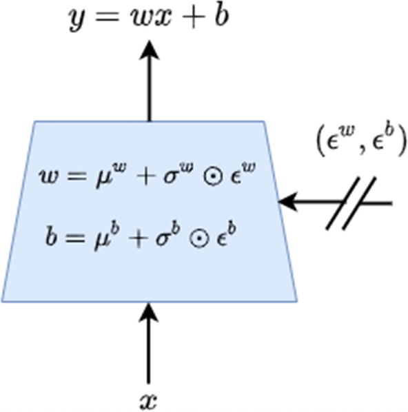
The usual linear layers are affine transformations as given by the following:
In noisy linear versions, we introduce random perturbations in the weights as given by the following:
In the previous equation, μw, σw, μb, and σb are the weights of the network that are learned. ϵw and ϵb are random noises that introduce randomness leading to exploration. Figure 6-9 gives a schematic diagram of the noisy version of the linear layer, which explains the equation we just talked about in the previous paragraph.
Figure 6-9
Noisy linear layer. The weights and biases are a linear combination of mean and standard deviation, which are learned just like the weights and biases in a regular linear layer
We will implement the factorized version as discussed in the paper where each element of the matrix is factored. Suppose we have p units of inputs and q units of output. Accordingly, we generate a p-size vector of Gaussian noise ϵi and a q-size vector of Gaussian noise ϵj. Each and can now be written as follows:
For factorized networks like the one we are using, we suggest you initialize the weights as follows:
Each element μi, j of μw and μb is sampled from uniform distribution in the range , where p is the number of input units.
Similarly, each element σi, j of σwand σb is initialized to a constant with the hyperparameter σ0 set to 0.5.
We create a noisy layer along the lines of the linear layer provided by PyTorch. We do so by extending nn.Module from PyTorch. It is a simple and standard implementation where you create your weight vectors in the init function. Then you write a forward function to take an input and transform it through a set of noisy linear and regular linear layers. You will also need some additional functions. In our case, we wrote a function called reset_noise to generate the noise ϵw and ϵb. This function internally uses a helper function called _noise. We also have a function reset_parameters to reset the parameters following the strategy outlined earlier. We could use a noisy net with DQN, DDQN, dueling DQN, and prioritized replay in various combinations. However, for the purpose of the walk-through, we will focus on using a regular replay buffer with DQN. We also train using the regular DQN approach and not DDQN. Listing 6-16 gives the code for the noisy linear.
The rest of the implementation remains same. The only difference now is that we have no ε-greedy selection in the function sample_actions of the DQN agent. We also have a reset_noise function to reset the noise after each batch. This is in line with the recommendations of the paper to decorrelate. Listing 6-17 contains the NoisyDQN version with the previous modifications. The rest of the implementation is similar to the vanilla DQN agent.
class NoisyDQN(nn.Module):
def __init__(self, state_shape, n_actions):
super(NoisyDQN, self).__init__()
self.n_actions = n_actions
self.state_shape = state_shape
state_dim = state_shape[0]
# a simple NN with state_dim as input vector (inout is state s)
# and self.n_actions as output vector of logits of q(s, a)
self.fc1 = NoisyLinear(state_dim, 64)
self.fc2 = NoisyLinear(64, 128)
self.fc3 = NoisyLinear(128, 32)
self.q = NoisyLinear(32, n_actions)
def forward(self, state_t):
# pass the state at time t through the newrok to get Q(s,a)
x = F.relu(self.fc1(state_t))
x = F.relu(self.fc2(x))
x = F.relu(self.fc3(x))
qvalues = self.q(x)
return qvalues
def get_qvalues(self, states):
# input is an array of states in numpy and outout is Qvals as numpy array
states = torch.tensor(states, device=device, dtype=torch.float32)
qvalues = self.forward(states)
return qvalues.data.cpu().numpy()
def sample_actions(self, qvalues):
# sample actions from a batch of q_values using greedy policy
batch_size, n_actions = qvalues.shape
best_actions = qvalues.argmax(axis=-1)
return best_actions
def reset_noise(self):
self.fc1.reset_noise()
self.fc2.reset_noise()
self.fc3.reset_noise()
self.q.reset_noise()
Listing 6-17
NoisyDQN Agent in PyTorch
Training a NoisyDQN in the CartPole environment produces the training curves, as given in Figure 6-10. We may not see any significant difference between this variant and DQN (or for that matter all the variants). The reason is that we are using a simple problem and training it for a short number of episodes. The idea in the book is to teach you the inner details of a specific variant. For a thorough study of the improvements and other observations, you are advised to refer to the original papers referenced. Also, once again we would like to emphasis that you should go through the accompanying Python notebooks in detail, and after you have grasped the details, you should try to code the example anew.
Figure 6-10
NoisyNet DQN training graph
You are also encouraged to try to code a noisy version of dueling DQN. Further, you could also try the DDQN variant of learning. In other words, with what we have learned so far, we could try following combinations:
DQN
DDQN (impacts how we learn)
Dueling DQN (impacts the architecture of training)
Dueling DDQN
Replace vanilla ReplayBuffer with prioritized replay buffer
Replace ε-exploration with NoisyNets in any of the previous approaches
Code all combinations on TensorFlow
Try many other Gym environments, making appropriate changes, if any, to the network
Run some of them on Atari, especially if you have access to a GPU machine
Categorical 51-Atom DQN (C51)
In a 2017 paper titled “A Distributional Perspective on Reinforcement Learning,”6 the authors argued in favor of the distributional nature of RL. Instead of looking at the expected values like the q-value, they looked at Z, a random distribution whose expectation is Q.
Up to now we have been outputting Q(s, a) values for an input state s. The number of units in the output were of size n_action. In a way, the output values were the expected Q(s, a) using the Monte Carlo technique of averaging over a number of samples to form an estimate of the actual expected value E[Q(s, a)].
In categorial 51-Atom DQN, for each Q(s, a) (n_action of them), we now produce an estimate of the distribution of Q(s, a) values: n_atom (51 to be precise) values for each Q(s, a). The network is now predicting the entire distribution modeled as a categorical probability distribution instead of just estimating the mean value of Q(s, a).
pi(s, a) is the probability that the action value at (s, a) will be zi.
We now have n_action * n_atom outputs, i.e., n_atom outputs for each value of n_action. Further, these outputs are probabilities. For one action, we have n_atom probabilities, and these are the probability of the q-value being in any one of the n_atom discrete values in the range V_min to V_max. You should refer to the previously mentioned paper for more details.
In the C51 version of distributional RL, the authors took ? to be 51 atoms (support points) over the values -10 to 10. We will use the same setup in the code. As these values are parameterized in the code, you are welcome to change them and explore the impact.
After the Bellman updates are applied, the values shift and may not fall on the 51 support points. There is a step of projection to bring back the probability distribution to the support points of 51 atoms.
The loss is also replaced from the mean squared error to cross-entropy loss. The agent is trained using an ε-greedy policy, similar to DQN. The whole math is fairly involved, and it will be a good exercise for you to go through the paper together with the code to link each code line with the specific detail in the paper. This is an important skill you as a practitioner of RL need to have.
Similar to the DQN approach, we have a class CategoricalDQN, which is the neural network through that takes the state s as input to produce the distribution Z of Q(s, a). There is a function to calculate the TD loss: td_loss_categorical_dqn. As discussed earlier, we need a projection step to bring the values back to the n_atom support points, which is carried out in the function compute_projection. Function compute_projection is used inside td_loss_categorical_dqn while calculating the loss calculation. The rest of the training remains the same as before.
Figure 6-11 gives the training curves for running this through the CartPole environment.
Figure 6-11
Categorical 51 Atom DQN (C51) training graph
Quantile Regression DQN
A little after the paper on the C51 algorithm was published in mid-2017, some of the original authors along with a few additional ones, all from DeepMind, came up with a variant that they called quantile regression DQN(QR-DQN). In a paper titled “Distributional Reinforcement Learning with Quantile Regression,”7 the authors used a slightly different approach than the original C51, but still within the same focus area of distribution RL.
Similar to the C51 approach of distributional RL, the QR-DQN approach also depended on using quantiles to predict the distribution of Q(s, a) instead of predicting an estimate of the average of Q(s, a). Both C51 and QR-DQN are variants of distributional RL and produced by scientists from DeepMind.
The C51 approach modeled the distribution of Qπ(s, a) named Zπ(s, a) as a categorical distribution of probability overfixed points in the range of Vmin to Vmax. The probability over these points was what was learned by the network. Such an approach resulted in the use of a projection step after the Bellman update to bring the new probabilities back to the fixed support points of n_atoms spread uniformly over Vmin to Vmax. While the result worked, there was a bit of disconnect with the theoretical basis on which the algorithm was derived.
In QR-DQN the approach is slightly different. The support points are still N, but now the probabilities were fixed to 1/N with the location of these points being learned by network. To quote the authors:
We “transpose” the parametrization from C51: whereas the former uses N fixed locations for its approximation distribution and adjusts their probabilities, we assign fixed, uniform probabilities to N adjustable locations.
The loss used in DQ DQN is that of quantile regression loss mixed with huber loss. This is called quantile huber loss; equations 9 and 10 in the referenced paper give the details. We are not showing the code listings here as we want you to read the paper and match the equations in the paper with the code in the notebook listing6_8_qr_dqn_pytorch.ipynb. The paper is dense with mathematics, and unless you are comfortable with advanced math, you should try to focus on the higher-level details of the approach.
In the 2018 paper by OpenAI titled “Hindsight Experience Replay,”8 the authors presented a sample efficient approach to learn in an environment where the rewards are sparse. The common approach is to shape the reward function in a way to guide the agents toward optimization. This is not generalizable.
Compared to RL agents, which learn from a successful outcome, humans seem to learn not just from that but also from unsuccessful outcomes. This is the basis of the idea proposed in the hindsight replay approach known as hindsight experience replay (HER). While HER can be combined with various RL approaches, in our code walk-through, we will use HER with dueling DQN, giving us HER-DQN.
In the HER approach, after an episode is played out, say an unsuccessful one, we form a secondary objective where the original goal is replaced with the last state before termination as a goal for this trajectory.
Say an episode has been played out: s0, s1, …. sT. Normally we store in the replay buffer a tuple of (st, at, r, st + 1, done). Let’s say the goal for this episode was g, which could not be achieved in this run. In the HER approach, we will store the following in the replay buffer:
(st| |g, at, r, st + 1| ∣ g, done)
(st| |g′, at, r(st, at, g′), st + 1| ∣ g′, done): Other state transitions based on synthetical goals like the last state of the episode as a subgoal, say g'. The reward is modified to show how the state transition st → st + 1 was good or bad for the subgoal of g′.
The original paper discusses various strategies for forming these subgoals. We will use the one called future, which is a replay with k random states that come from the same episode as the transition being replayed and were observed after it.
We also use a different kind of environment from our past notebooks. We will use an environment of a bit-flipping experiment. Say you have a vector with n-bits, each being a binary in the range {0,1}. Therefore, there are 2n combinations possible. At reset, the environment starts in a n-bit configuration chosen randomly, and the goal is also randomly picked to be some different n-bit configuration. Each action is to flip a bit. The bit to be flipped is the policy π(a| s) that the agent is trying to learn. An episode ends if the agent is able to find the right configuration matching the goal or when the agent has exhausted n actions in an episode. Listing 6-18 shows the code for the environment. The complete code is in notebook listing6_9_her_dqn_pytorch.ipynb.
We have implemented our own render and step functions so that the interface of our environment remains similar to the ones in Gym and so that we can use our previously developed machinery. We also have a custom function compute_reward to return the reward and done flags when given the input of a state and a goal.
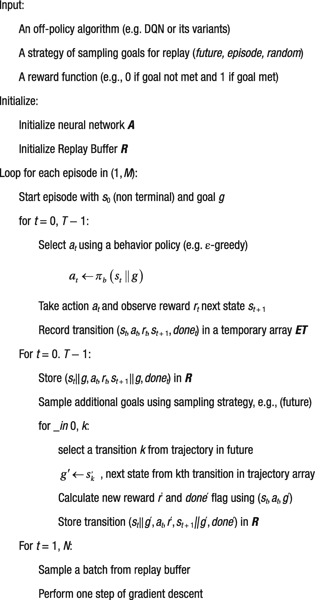
The authors show that with a regular DQN, where the state (configuration of n-bits) is represented as a deep network, it is almost impossible for a regular DQN agent to learn beyond 15-digit combinations. However, coupled with the HER-DQN approach, the agent is able to learn easily even for large-digit combinations like 50 or so. In Figure 6-13 we give the complete pseudocode from the paper with certain modifications to make it match with our notations.
Hindsight Experience Replay (HER)
Figure 6-13
HER using a future strategy
We use dueling DQN. The most interesting part of the code is the implementation of the HER algorithm as per the pseudocode given in Figure 6-13. Listing 6-19 is a line-by-line implementation of that pseudocode.
In the code, we use the previously coded td_loss_dqn function to compute the TD loss and take a gradient step. We also start with a very exploratory behavior policy with ε=0.2 and slowly reduce it to zero, halfway through the training. The rest of the code matches line by line with the pseudocode in Figure 6-13.
Figure 6-14 shows the training curve. For a 50-bit BitFlipping environment, the agent with HER is able to successfully solve the environment 100 percent of the time. Remember, the environment starts with a random combination of 50 bits as a starting point and another random combination as the goal. The agent has a maximum of 50 flipping moves to reach the goal combination. An exhaustive search would require the agent to try each of the 250 combinations except the one it started with initially.
Figure 6-14
Success rate graph: bit flipping environment with HER using a future strategy
This brings us to the end of discussion on HER as well as to the end of chapter.
Summary
This was a fairly long chapter where we looked at DQN and most of its popular and recent variants.
We started with a quick recap of Q-learning and the derivation of the update equation for DQN. We then looked at the implementation of DQN in both PyTorch and TensorFlow for a simple CartPole environment. After this we looked at the Atari games, the original inspiration in 2013, to be able to use deep learning in the context of reinforcement learning. We looked at the additional preprocessing steps and changes in the network from a linear one to one based on convolutional layers.
Next, we talked about prioritized replay where the samples from the buffer are picked based on a certain importance score assigned to them proportional to the magnitude of the TD error.
Following this, we revisited double Q-learning in the context of DQN, known as double DQN. This is an approach that impacts the way learning takes place and attempts to reduce the maximization bias.
We then looked at dueling DQN in which two networks with an initial shared network were used. This was followed by NoisyNets in which ε-greedy exploration was replaced by noisy layers.
Next, we looked at two flavors of distributional RL under which the network produced Z, a distribution of q-values. Instead of producing the expected action-value Q(S, A), it outputs the whole distribution, specifically a categorical distribution. We also saw the use of the projection step and losses like cross entropy and quantile huber loss.
The last section was on hindsight experience replay, which addresses learning in environments with sparse rewards. Previous learning approaches were centered around learning only from successful outcomes, but hindsight replay allows us to learn from unsuccessful outcomes as well.
Many of algorithms and approaches we saw in this chapter are state-of-the-art research. You will gain a lot by looking at the original papers as well as going through the code line by line. We have also suggested the various combinations that you could try to code to further cement the concepts in your mind.
This chapter concludes our exploration of value-based methods where we learn a policy by first learning with V or Q functions and then using these to find an optimal policy. In the next chapter, we will switch to policy-based methods where we find the optimal policy without the involvement of the intermediary step of learning V/Q functions.
![$$ Qleft({S}_t,{A}_t
ight)leftarrow Qleft({S}_t,{A}_t
ight)+alpha ast left[{R}_{t+1}+gamma ast {}_{akern0.5em }{}^{mathit{max}}Qleft({S}_{t+1},{A}_{t+1}
ight)-Qleft({S}_t,{A}_t
ight)
ight] $$](https://imgdetail.ebookreading.net/202109/3/9781484268094/9781484268094__9781484268094__files__images__502835_1_En_6_Chapter__502835_1_En_6_Chapter_TeX_Equ1.png)
![$$ {w}_{t+1}={w}_t+alpha .kern0.5em frac{1}{N}sum limits_{i=1}^Nleft[{r}_i+gamma {mathit{max}}_{a_i^{prime }}overset{sim }{q}left({s}_i^{prime },{a}_i^{prime };{w_t}^{-}
ight)-hat{q}left({s}_i,{a}_i;w
ight)
ight].{
abla}_w hat{q}left({s}_i,{a}_i;w
ight) $$](https://imgdetail.ebookreading.net/202109/3/9781484268094/9781484268094__9781484268094__files__images__502835_1_En_6_Chapter__502835_1_En_6_Chapter_TeX_Equ2.png)
![$$ L=frac{1}{N}{sum}_{i=1}^N{left[{r}_i+left(left(1- don{e}_i
ight).upgamma .underset{a_i^{prime }}{max}hat{q}left({s}_i^{prime },{a}_i^{prime };{w}_t^{-}
ight)
ight)hbox{--} hat{q}left({s}_i,{a}_i;{w}_t
ight)
ight]}^2 $$](https://imgdetail.ebookreading.net/202109/3/9781484268094/9781484268094__9781484268094__files__images__502835_1_En_6_Chapter__502835_1_En_6_Chapter_TeX_Equ3.png)
![$$ {
abla}_{mathrm{w}}mathrm{L}=-frac{1}{mathrm{N}}{sum}_{mathrm{i}=1}^{mathrm{N}}left[{mathrm{r}}_{mathrm{i}}+left(left(1-mathrm{don}{mathrm{e}}_{mathrm{i}}
ight).upgamma .underset{{mathrm{a}}_{mathrm{i}}^{prime }}{max}hat{mathrm{q}}left({mathrm{s}}_{mathrm{i}}^{prime },{mathrm{a}}_{mathrm{i}}^{prime };{mathrm{w}}_{mathrm{t}}^{-}
ight)
ight)hbox{--} hat{mathrm{q}}left({mathrm{s}}_{mathrm{i}},{mathrm{a}}_{mathrm{i}};{mathrm{w}}_{mathrm{t}}
ight)
ight]
abla hat{mathrm{q}}left({mathrm{s}}_{mathrm{i}},{mathrm{a}}_{mathrm{i}};{mathrm{w}}_{mathrm{t}}
ight) $$](https://imgdetail.ebookreading.net/202109/3/9781484268094/9781484268094__9781484268094__files__images__502835_1_En_6_Chapter__502835_1_En_6_Chapter_TeX_Equ4.png)

 . That’s one of the primary reasons to use packages like PyTorch and TensorFlow, which automatically calculate gradients based on the operations performed to calculate the loss metric L. We just need a function to calculate that metric L. This is done by the function compute_td_loss. It takes in a batch of (states, actions, rewards, next_states, done_flags). It also takes in the discount parameter γ as well as the agent/online and target networks. The function then computes loss L as per equation (6.3). Listing 6-5 gives the implementation in PyTorch, and Listing 6-6 gives it in TensorFlow.
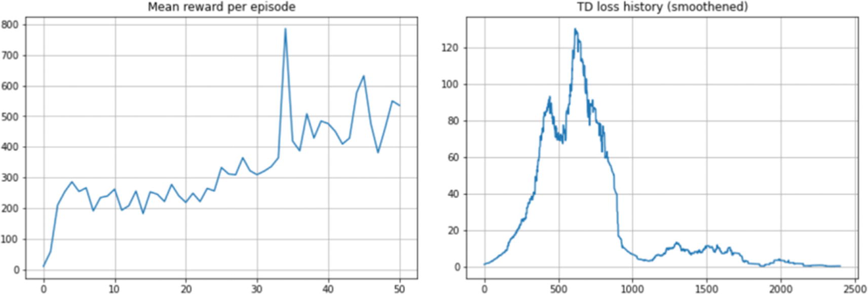


 , where rank(i) is the rank of transition(i) when the replay buffer transitions are sorted based on |δi|. In our code example, we will be using the first approach, which is called proportional prioritization
.
, where rank(i) is the rank of transition(i) when the replay buffer transitions are sorted based on |δi|. In our code example, we will be using the first approach, which is called proportional prioritization
.

 to ensure that the weights stay within bounds.
![$$ L=frac{1}{N}{sum}_{i=1}^N{left[left({r}_i+left(left(1- don{e}_i
ight).upgamma .underset{a_i^{prime }}{max}hat{q}left({s}_i^{prime },{a}_i^{prime };{w}_t^{-}
ight)
ight)hbox{--} hat{q}left({s}_i,{a}_i;{w}_t
ight)
ight).{w}_i
ight]}^2 $$](https://imgdetail.ebookreading.net/202109/3/9781484268094/9781484268094__9781484268094__files__images__502835_1_En_6_Chapter__502835_1_En_6_Chapter_TeX_Equ11.png)


 , first for selecting the best action and then for getting the q-value for that action. This is what causes maximization bias. The authors of the paper suggested an approach that they called double DQN (DDQN) where the weight for selecting the best action,
  , comes from the online network with weight wt and then the target network with weight
  is used to select the q-value for that best action. This change results in the updated TD target as follows:
![$$ L=frac{1}{N}{sum}_{i=1}^N{left[{r}_i+left(left(1- don{e}_i
ight).upgamma .hat{q}left({s}_i^{prime }, argma{x}_{a^{prime }}hat{q}left({s}_i^{prime },{a}^{prime };{w}_t
ight);{w}_t^{-}
ight)
ight)hbox{--} hat{q}left({s}_i,{a}_i;{w}_t
ight)
ight]}^2 $$](https://imgdetail.ebookreading.net/202109/3/9781484268094/9781484268094__9781484268094__files__images__502835_1_En_6_Chapter__502835_1_En_6_Chapter_TeX_Equ12.png)
![$$ {v}_{pi }(s)={E}_{pi}left[ {G}_t
ight| {S}_t=s Big] $$](https://imgdetail.ebookreading.net/202109/3/9781484268094/9781484268094__9781484268094__files__images__502835_1_En_6_Chapter__502835_1_En_6_Chapter_TeX_Equd.png)
![$$ {q}_{pi}left(s,a
ight)={E}_{pi } left[ {G}_t
ight| {S}_t=s,{A}_t=a Big] $$](https://imgdetail.ebookreading.net/202109/3/9781484268094/9781484268094__9781484268094__files__images__502835_1_En_6_Chapter__502835_1_En_6_Chapter_TeX_Eque.png)


 , and finally w3 corresponds to the part of network that predicts advantage
  . Figure 6-7 shows a representative network architecture.
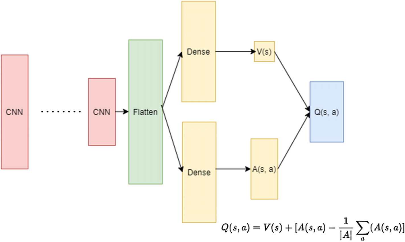


 of the matrix is factored. Suppose we have p units of inputs and q units of output. Accordingly, we generate a p-size vector of Gaussian noise ϵi and a q-size vector of Gaussian noise ϵj. Each
  and
and  can now be written as follows:


![$$ Uleft[-frac{1}{sqrt{p}},frac{1}{sqrt{p}}
ight] $$](https://imgdetail.ebookreading.net/202109/3/9781484268094/9781484268094__9781484268094__files__images__502835_1_En_6_Chapter__502835_1_En_6_Chapter_TeX_IEq12.png) , where p is the number of input units.
, where p is the number of input units. with the hyperparameter σ0 set to 0.5.
 of the actual expected value E[Q(s, a)].