10
Policy Gradient Method
In the previous chapters, we learned how to use value-based reinforcement learning algorithms to compute the optimal policy. That is, we learned that with value-based methods, we compute the optimal Q function iteratively and from the optimal Q function, we extract the optimal policy. In this chapter, we will learn about policy-based methods, where we can compute the optimal policy without having to compute the optimal Q function.
We will start the chapter by looking at the disadvantages of computing a policy from the Q function, and then we will learn how policy-based methods learn the optimal policy directly without computing the Q function. Next, we will examine one of the most popular policy-based methods, called the policy gradient. We will first take a broad overview of the policy gradient algorithm, and then we will learn more about it in detail.
Going forward, we will also learn how to derive the policy gradient step by step and examine the algorithm of the policy gradient method in more detail. At the end of the chapter, we will learn about the variance reduction techniques in the policy gradient method.
In this chapter, we will learn the following topics:
- Why policy-based methods?
- Policy gradient intuition
- Deriving the policy gradient
- Algorithm of policy gradient
- Policy gradient with reward-to-go
- Policy gradient with baseline
- Algorithm of policy gradient with baseline
Why policy-based methods?
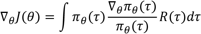
The objective of reinforcement learning is to find the optimal policy, which is the policy that provides the maximum return. So far, we have learned several different algorithms for computing the optimal policy, and all these algorithms have been value-based methods. Wait, what are value-based methods? Let's recap what value-based methods are, and the problems associated with them, and then we will learn about policy-based methods. Recapping is always good, isn't it?
With value-based methods, we extract the optimal policy from the optimal Q function (Q values), meaning we compute the Q values of all state-action pairs to find the policy. We extract the policy by selecting an action in each state that has the maximum Q value. For instance, let's say we have two states s0 and s1 and our action space has two actions; let the actions be 0 and 1. First, we compute the Q value of all the state-action pairs, as shown in the following table. Now, we extract policy from the Q function (Q values) by selecting action 0 in state s0 and action 1 in state s1 as they have the maximum Q value:

Table 10.1: Q table
Later, we learned that it is difficult to compute the Q function when our environment has a large number of states and actions as it would be expensive to compute the Q values of all possible state-action pairs. So, we resorted to the Deep Q Network (DQN). In DQN, we used a neural network to approximate the Q function (Q value). Given a state, the network will return the Q values of all possible actions in that state. For instance, consider the grid world environment. Given a state, our DQN will return the Q values of all possible actions in that state. Then we select the action that has the highest Q value. As we can see in Figure 10.1, given state E, DQN returns the Q value of all possible actions (up, down, left, right). Then we select the right action in state E since it has the maximum Q value:

Figure 10.1: DQN
Thus, in value-based methods, we improve the Q function iteratively, and once we have the optimal Q function, then we extract optimal policy by selecting the action in each state that has the maximum Q value.
One of the disadvantages of the value-based method is that it is suitable only for discrete environments (environments with a discrete action space), and we cannot apply value-based methods in continuous environments (environments with a continuous action space).
We have learned that a discrete action space has a discrete set of actions; for example, the grid world environment has discrete actions (up, down, left, and right) and the continuous action space consists of actions that are continuous values, for example, controlling the speed of a car.
So far, we have only dealt with a discrete environment where we had a discrete action space, so we easily computed the Q value of all possible state-action pairs. But how can we compute the Q value of all possible state-action pairs when our action space is continuous? Say we are training an agent to drive a car and say we have one continuous action in our action space. Let the action be the speed of the car and the value of the speed of the car ranges from 0 to 150 kmph. In this case, how can we compute the Q value of all possible state-action pairs with the action being a continuous value?
In this case, we can discretize the continuous actions into speed (0 to 10) as action 1, speed (10 to 20) as action 2, and so on. After discretization, we can compute the Q value of all possible state-action pairs. However, discretization is not always desirable. We might lose several important features and we might end up in an action space with a huge set of actions.
Most real-world problems have continuous action space, say, a self-driving car, or a robot learning to walk and more. Apart from having a continuous action space they also have a high dimension. Thus, the DQN and other value-based methods cannot deal with the continuous action space effectively.
So, we use the policy-based methods. With policy-based methods, we don't need to compute the Q function (Q values) to find the optimal policy; instead, we can compute them directly. That is, we don't need the Q function to extract the policy. Policy-based methods have several advantages over value-based methods, and they can handle both discrete and continuous action spaces.
We learned that DQN takes care of the exploration-exploitation dilemma by using the epsilon-greedy policy. With the epsilon-greedy policy, we either select the best action with the probability 1-epsilon or a random action with the probability epsilon. Most policy-based methods use a stochastic policy. We know that with a stochastic policy, we select actions based on the probability distribution over the action space, which allows the agent to explore different actions instead of performing the same action every time. Thus, policy-based methods take care of the exploration-exploitation trade-off implicitly by using a stochastic policy. However, there are several policy-based methods that use a deterministic policy as well. We will learn more about them in the upcoming chapters.
Okay, how do policy-based methods work, exactly? How do they find an optimal policy without computing the Q function? We will learn about this in the next section. Now that we have a basic understanding of what a policy gradient method is, and also the disadvantages of value-based methods, in the next section we will learn about a fundamental and interesting policy-based method called policy gradient.
Policy gradient intuition
Policy gradient is one of the most popular algorithms in deep reinforcement learning. As we have learned, policy gradient is a policy-based method by which we can find the optimal policy without computing the Q function. It finds the optimal policy by directly parameterizing the policy using some parameter ![]() .
.
The policy gradient method uses a stochastic policy. We have learned that with a stochastic policy, we select an action based on the probability distribution over the action space. Say we have a stochastic policy ![]() , then it gives the probability of taking an action a given the state s. It can be denoted by
, then it gives the probability of taking an action a given the state s. It can be denoted by 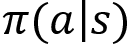 . In the policy gradient method, we use a parameterized policy, so we can denote our policy as
  , where
 ![]() indicates that our policy is parameterized.
indicates that our policy is parameterized.
Wait! What do we mean when we say a parameterized policy? What is it exactly? Remember with DQN, we learned that we parameterize our Q function to compute the Q value? We can do the same here, except instead of parameterizing the Q function, we will directly parameterize the policy to compute the optimal policy. That is, we can use any function approximator to learn the optimal policy, and ![]() is the parameter of our function approximator. We generally use a neural network as our function approximator. Thus, we have a policy
is the parameter of our function approximator. We generally use a neural network as our function approximator. Thus, we have a policy ![]() parameterized by
parameterized by ![]() where
where ![]() is the parameter of the neural network.
is the parameter of the neural network.
Say we have a neural network with a parameter ![]() . First, we feed the state of the environment as an input to the network and it will output the probability of all the actions that can be performed in the state. That is, it outputs a probability distribution over an action space. We have learned that with policy gradient, we use a stochastic policy. So, the stochastic policy selects an action based on the probability distribution given by the neural network. In this way, we can directly compute the policy without using the Q function.
. First, we feed the state of the environment as an input to the network and it will output the probability of all the actions that can be performed in the state. That is, it outputs a probability distribution over an action space. We have learned that with policy gradient, we use a stochastic policy. So, the stochastic policy selects an action based on the probability distribution given by the neural network. In this way, we can directly compute the policy without using the Q function.
Let's understand how the policy gradient method works with an example. Let's take our favorite grid world environment for better understanding. We know that in the grid world environment our action space has four possible actions: up, down, left, and right.
Given any state as an input, the neural network will output the probability distribution over the action space. That is, as shown in Figure 10.2, when we feed the state E as an input to the network, it will return the probability distribution over all actions in our action space. Now, our stochastic policy will select an action based on the probability distribution given by the neural network. So, it will select action up 10% of the time, down 10% of the time, left 10% of the time, and right 70% of the time:
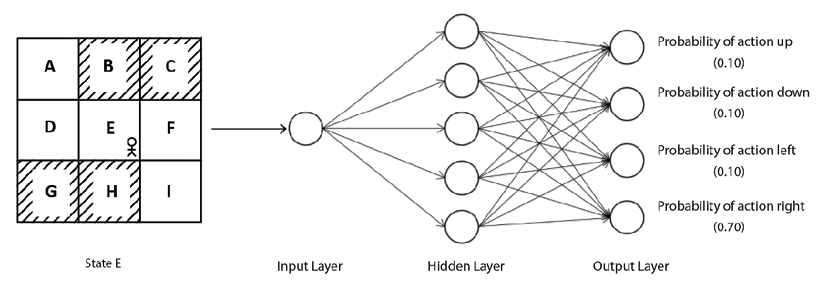
Figure 10.2: A policy network
We should not get confused with the DQN and the policy gradient method. With DQN, we feed the state as an input to the network, and it returns the Q values of all possible actions in that state, then we select an action that has a maximum Q value. But in the policy gradient method, we feed the state as input to the network, and it returns the probability distribution over an action space, and our stochastic policy uses the probability distribution returned by the neural network to select an action.
Okay, in the policy gradient method, the network returns the probability distribution (action probabilities) over the action space, but how accurate are the probabilities? How does the network learn?
Unlike supervised learning, here we will not have any labeled data to train our network. So, our network does not know the correct action to perform in the given state; that is, the network does not know which action gives the maximum reward. So, the action probabilities given by our neural network will not be accurate in the initial iterations, and thus we might get a bad reward.
But that is fine. We simply select the action based on the probability distribution given by the network, store the reward, and move to the next state until the end of the episode. That is, we play an episode and store the states, actions, and rewards. Now, this becomes our training data. If we win the episode, that is, if we get a positive return or high return (the sum of the rewards of the episode), then we increase the probability of all the actions that we took in each state until the end of the episode. If we get a negative return or low return, then we decrease the probability of all the actions that we took in each state until the end of the episode.
Let's understand this with an example. Say we have states s1 to s8 and our goal is to reach state s8. Say our action space consists of only two actions: left and right. So, when we feed any state to the network, then it will return the probability distribution over the two actions.
Consider the following trajectory (episode) ![]() , where we select an action in each state based on the probability distribution returned by the network using a stochastic policy:
, where we select an action in each state based on the probability distribution returned by the network using a stochastic policy:
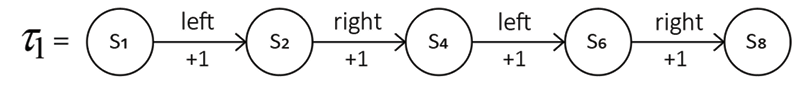
Figure 10.3: Trajectory ![]()
The return of this trajectory is  . Since we got a positive return, we increase the probabilities of all the actions that we took in each state until the end of the episode. That is, we increase the probabilities of action left in s1, action right in s2, and so on until the end of the episode.
Let's suppose we generate another trajectory ![]() , where we select an action in each state based on the probability distribution returned by the network using a stochastic policy, as shown in Figure 10.4:
, where we select an action in each state based on the probability distribution returned by the network using a stochastic policy, as shown in Figure 10.4:

Figure 10.4: Trajectory ![]()
The return of this trajectory is  . Since we got a negative return, we decrease the probabilities of all the actions that we took in each state until the end of the episode. That is, we will decrease the probabilities of action right in s1, action right in s3, and so on until the end of the episode.
Okay, but how exactly do we increase and decrease these probabilities? We learned that if the return of the trajectory is positive, then we increase the probabilities of all actions in the episode, else we decrease it. How can we do this exactly? This is where backpropagation helps us. We know that we train the neural network by backpropagation.
So, during backpropagation, the network calculates gradients and updates the parameters of the network ![]() . Gradients updates are in such a way that actions yielding high return will get high probabilities and actions yielding low return will get low probabilities.
. Gradients updates are in such a way that actions yielding high return will get high probabilities and actions yielding low return will get low probabilities.
In a nutshell, in the policy gradient method, we use a neural network to find the optimal policy. We initialize the network parameter ![]() with random values. We feed the state as an input to the network and it will return the action probabilities. In the initial iteration, since the network is not trained with any data, it will give random action probabilities. But we select actions based on the action probability distribution given by the network and store the state, action, and reward until the end of the episode. Now, this becomes our training data. If we win the episode, that is, if we get a high return, then we assign high probabilities to all the actions of the episode, else we assign low probabilities to all the actions of the episode.
with random values. We feed the state as an input to the network and it will return the action probabilities. In the initial iteration, since the network is not trained with any data, it will give random action probabilities. But we select actions based on the action probability distribution given by the network and store the state, action, and reward until the end of the episode. Now, this becomes our training data. If we win the episode, that is, if we get a high return, then we assign high probabilities to all the actions of the episode, else we assign low probabilities to all the actions of the episode.
Since we are using a neural network to find the optimal policy, we can call this neural network a policy network. Now that we have a basic understanding of the policy gradient method, in the next section, we will learn how exactly the neural network finds the optimal policy; that is, we will learn how exactly the gradient computation happens and how we train the network.
Understanding the policy gradient
In the last section, we learned that, in the policy gradient method, we update the gradients in such a way that actions yielding a high return will get a high probability, and actions yielding a low return will get a low probability. In this section, we will learn how exactly we do that.
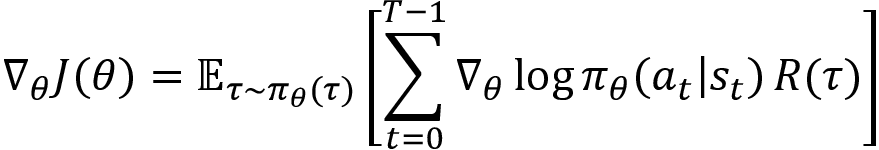
The goal of the policy gradient method is to find the optimal parameter ![]() of the neural network so that the network returns the correct probability distribution over the action space. Thus, the objective of our network is to assign high probabilities to actions that maximize the expected return of the trajectory. So, we can write our objective function J as:
of the neural network so that the network returns the correct probability distribution over the action space. Thus, the objective of our network is to assign high probabilities to actions that maximize the expected return of the trajectory. So, we can write our objective function J as:
In the preceding equation, the following applies:
 is the trajectory.
 denotes that we are sampling the trajectory based on the policy
  given by network parameterized by
  .
. is the return of the trajectory
  .
.
Thus, maximizing our objective function maximizes the return of the trajectory. How can we maximize the preceding objective function? We generally deal with minimization problems, where we minimize the loss function (objective function) by calculating the gradients of our loss function and updating the parameter using gradient descent. But here, our goal is to maximize the objective function, so we calculate the gradients of our objective function and perform gradient ascent. That is:

Where  implies the gradients of our objective function. Thus, we can find the optimal parameter
 ![]() of our network using gradient ascent.
of our network using gradient ascent.
The gradient  is derived as
  . We will learn how exactly we derived this gradient in the next section. In this section, let's focus only on getting a good fundamental understanding of the policy gradient.
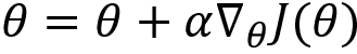
We learned that we update our network parameter with:
Substituting the value of gradient, our parameter update equation becomes:

In the preceding equation, the following applies:
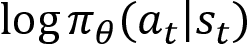 represents the log probability of taking an action a given the state s at a time t.
 represents the return of the trajectory.
We learned that we update the gradients in such a way that actions yielding a high return will get a high probability, and actions yielding a low return will get a low probability. Let's now see how exactly we are doing that.
Case 1:
Suppose we generate an episode (trajectory) using the policy ![]() , where
, where ![]() is the parameter of the network. After generating the episode, we compute the return of the episode. If the return of the episode is negative, say -1, that is,
is the parameter of the network. After generating the episode, we compute the return of the episode. If the return of the episode is negative, say -1, that is, 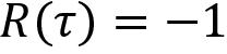 , then we decrease the probability of all the actions that we took in each state until the end of the episode.
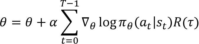
We learned that our parameter update equation is given as:
In the preceding equation, multiplying  by the negative return implies that we are decreasing the log probability of action at in state st. Thus, we perform a negative update. That is:
For each step in the episode, t = 0, . . ., T-1, we update the parameter ![]() as:
as:

It implies that we are decreasing the probability of all the actions that we took in each state until the end of the episode.
Case 2:
Suppose we generate an episode (trajectory) using the policy ![]() , where
, where ![]() is the parameter of the network. After generating the episode, we compute the return of the episode. If the return of the episode is positive, say +1, that is,
is the parameter of the network. After generating the episode, we compute the return of the episode. If the return of the episode is positive, say +1, that is, 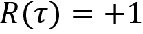 , then we increase the probability of all the actions that we took in each state until the end of the episode.
We learned that our parameter update equation is given as:
In the preceding equation, multiplying  by the positive return, , means that we are increasing the log probability of action at in the state st. Thus, we perform a positive update. That is:
For each step in the episode, t = 0, . . ., T-1, we update the parameter ![]() as:
as:

Thus, if we get a positive return then we increase the probability of all the actions performed in that episode, else we will decrease the probability.
We learned that, for each step in the episode, t = 0, . . ., T-1, we update the parameter ![]() as:
as:
We can simply denote the preceding equation as:
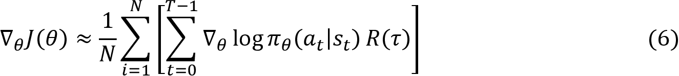
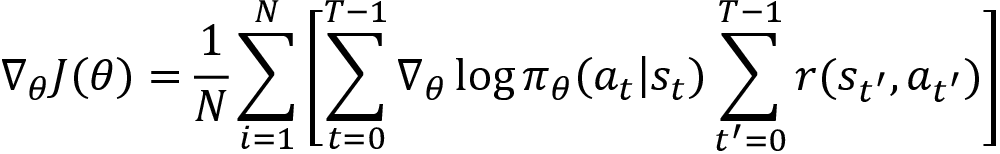
Thus, if the episode (trajectory) gives a high return, we will increase the probabilities of all the actions of the episode, else we decrease the probabilities. We learned that . What about that expectation? We have not included that in our update equation yet. When we looked at the Monte Carlo method, we learned that we can approximate the expectation using the average. Thus, using the Monte Carlo approximation method, we change the expectation term to the sum over N trajectories. So, our update equation becomes:
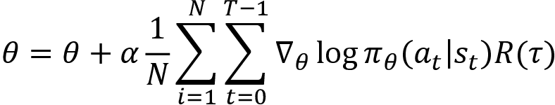
It shows that instead of updating the parameter based on a single trajectory, we collect a set of N trajectories following the policy ![]() and update the parameter based on the average value, that is:
and update the parameter based on the average value, that is:
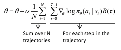
Thus, first, we collect N number of trajectories  following the policy
 ![]() and compute the gradient as:
and compute the gradient as:

And then we update our parameter as:
But we can't find the optimal parameter ![]() by updating the parameter for just one iteration. So, we repeat the previous step for many iterations to find the optimal parameter.
by updating the parameter for just one iteration. So, we repeat the previous step for many iterations to find the optimal parameter.
Now that we have a fundamental understanding of how policy gradient method work, in the next section, we will learn how to derive the policy gradient  . After that, we will learn about the policy gradient algorithm in detail step by step.
Deriving the policy gradient
In this section, we will get into more details and learn how to compute the gradient 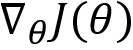 and how it is equal to
  .
.
Let's deep dive into the interesting math and see how to calculate the derivative of our objective function J with respect to the model parameter ![]() in simple steps. Don't get intimidated by the upcoming equations, it's actually a pretty simple derivation. Before going ahead, let's revise some math prerequisites in order to understand our derivation better.
in simple steps. Don't get intimidated by the upcoming equations, it's actually a pretty simple derivation. Before going ahead, let's revise some math prerequisites in order to understand our derivation better.
Definition of the expectation:
Let X be a discrete random variable whose probability mass function (pmf) is given as p(x). Let f be a function of a discrete random variable X. Then the expectation of a function f(X) can be defined as:

Let X be a continuous random variable whose probability density function (pdf) is given as p(x). Let f be a function of a continuous random variable X. Then the expectation of a function f(X) can be defined as:

A log derivative trick is given as:

We learned that the objective of our network is to maximize the expected return of the trajectory. Thus, we can write our objective function J as:

In the preceding equation, the following applies:
 is the trajectory.
 shows that we are sampling the trajectory based on the policy
  given by network parameterized by
  .
. is the return of the trajectory.
As we can see, our objective function, equation (4), is in the expectation form. From the definition of the expectation given in equation (2), we can expand the expectation and rewrite equation (4) as:

Now, we calculate the derivative of our objective function J with respect to ![]() :
:
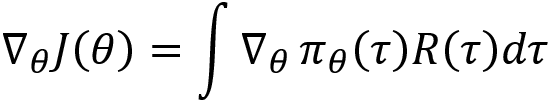
Multiplying and dividing by  , we can write:
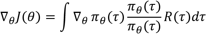
Rearranging the preceding equation, we can write:
From equation (3), substituting 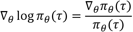 in the preceding equation, we can write:

From the definition of expectation given in equation (2), we can rewrite the preceding equation in expectation form as:

The preceding equation gives us the gradient of the objective function. But we still haven't solved the equation yet. As we can see, in the preceding equation we have the term 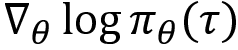 . Now we will see how we can compute that.
The probability distribution of trajectory can be given as:

Where p(s0) is the initial state distribution. Taking the log on both sides, we can write:
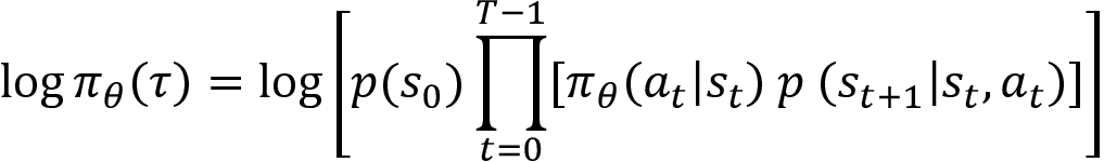
We know that the log of a product is equal to the sum of the logs, that is,  . Applying this log rule to the preceding equation, we can write:
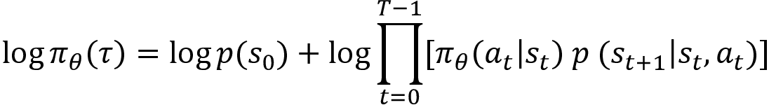
Again, we apply the same rule, log of product = sum of logs, and change the log ![]() to
to ![]() logs, as shown here:
logs, as shown here:
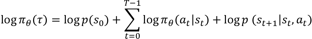
Now, we compute the derivate with respect to ![]() :
:
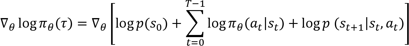
Note that we are calculating derivative with respect to ![]() and, as we can see in the preceding equation, the first and last term on the right-hand side (RHS) does not depend on the
and, as we can see in the preceding equation, the first and last term on the right-hand side (RHS) does not depend on the ![]() , and so they will become zero while calculating derivative. Thus our equation becomes:
, and so they will become zero while calculating derivative. Thus our equation becomes:
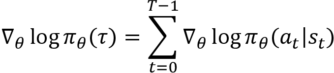
Now that we have found the value for  , substituting this in equation (5) we can write:
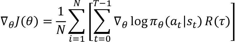
That's it. But can we also get rid of that expectation? Yes! We can use a Monte Carlo approximation method and change the expectation to the sum over N trajectories. So, our final gradient becomes:
Equation (6) shows that instead of updating a parameter based on a single trajectory, we collect N number of trajectories and update the parameter based on its average value over N trajectories.
Thus, after computing the gradient, we can update our parameter as:
Thus, in this section, we have learned how to derive a policy gradient. In the next section, we will get into more details and learn about the policy gradient algorithm step by step.
Algorithm – policy gradient
The policy gradient algorithm we discussed so far is often called REINFORCE or Monte Carlo policy gradient. The algorithm of the REINFORCE method is given in the following steps:
- Initialize the network parameter
 with random values
 - Generate N trajectories
 following the policy
- Compute the return of the trajectory

- Compute the gradients
- Update the network parameter as
- Repeat steps 2 to 5 for several iterations
As we can see from this algorithm, the parameter ![]() is getting updated in every iteration. Since we are using the parameterized policy
is getting updated in every iteration. Since we are using the parameterized policy ![]() , our policy is getting updated in every iteration.
, our policy is getting updated in every iteration.
The policy gradient algorithm we just learned is an on-policy method, as we are using only a single policy. That is, we are using a policy to generate trajectories and we are also improving the same policy by updating the network parameter ![]() in every iteration.
in every iteration.
We learned that with the policy gradient method (the REINFORCE method), we use a policy network that returns the probability distribution over the action space and then we select an action based on the probability distribution returned by our network using a stochastic policy. But this applies only to a discrete action space, and we use categorical policy as our stochastic policy.
What if our action space is continuous? That is, when the action space is continuous, how can we select actions? Here, our policy network cannot return the probability distribution over the action space as the action space is continuous. So, in this case, our policy network will return the mean and variance of the action as output, and then we generate a Gaussian distribution using this mean and variance and select an action by sampling from this Gaussian distribution using the Gaussian policy. We will learn more about this in the upcoming chapters. Thus, we can apply the policy gradient method to both discrete and continuous action spaces. Next, we will look at two methods to reduce the variance of policy gradient updates.
Variance reduction methods
In the previous section, we learned one of the simplest policy gradient methods, called the REINFORCE method. One major issue we face with the policy gradient method we learned in the previous section is that the gradient,  , will have high variance in each update. The high variance is basically due to the major difference in the episodic returns. That is, we learned that policy gradient is the on-policy method, which means that we improve the same policy with which we are generating episodes in every iteration. Since the policy is getting improved on every iteration, our return varies greatly in each episode and it introduces a high variance in the gradient updates. When the gradients have high variance, then it will take a lot of time to attain convergence.
Thus, now we will learn the following two important methods to reduce the variance:
- Policy gradients with reward-to-go (causality)
- Policy gradients with baseline
Policy gradient with reward-to-go
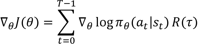
We learned that the policy gradient is computed as:
Now, we make a small change in the preceding equation. We know that the return of the trajectory is the sum of the rewards of that trajectory, that is:
Instead of using the return of trajectory  , we use something called reward-to-go Rt. Reward-to-go is basically the return of the trajectory starting from state st. That is, instead of multiplying the log probabilities by the return of the full trajectory
  in every step of the episode, we multiply them by the reward-to-go Rt. The reward-to-go implies the return of the trajectory starting from state st. But why do we have to do this? Let's understand this in more detail with an example.
We learned that we generate N number of trajectories and compute the gradient as:
For better understanding, let's take only one trajectory by setting N=1, so we can write:
Say, we generated the following trajectory with the policy ![]() :
:
Figure 10.5: Trajectory
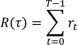
The return of the preceding trajectory is  .
.
Now, we can compute gradient as:

As we can observe from the preceding equation, in every step of the episode, we are multiplying the log probability of the action by the return of the full trajectory , which is 2 in the preceding example.
Let's suppose we want to know how good the action right is in the state s2. If we understand that the action right is a good action in the state s2, then we can increase the probability of moving right in the state s2, else we decrease it. Okay, how can we tell whether the action right is good in the state s2? As we learned in the previous section (when discussing the REINFORCE method), if the return of the trajectory is high, then we increase the probability of the action right in the state s2, else we decrease it.
But we don't have to do that now. Instead, we can compute the return (the sum of the rewards of the trajectory) only starting from the state s2 because there is no use in including all the rewards that we obtain from the trajectory before taking the action right in the state s2. As Figure 10.6 shows, including all the rewards that we obtain before taking the action right in the state s2 will not help us understand how good the action right is in the state s2:
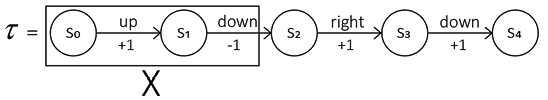
Figure 10.6: Trajectory
Thus, instead of taking the complete return of the trajectory in all the steps of the episode, we use reward-to-go Rt, which is the return of the trajectory starting from the state st.
Thus, now we can write:

Where R0 indicates the return of the trajectory starting from the state s0, R1 indicates the return of the trajectory starting from the state s1, and so on. If R0 is high value, then we increase the probability of the action up in the state s0, else we decrease it. If R1 is high value, then we increase the probability of the action down in the state s1, else we decrease it.
Thus, now, we can define the reward-to-go as:
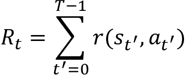
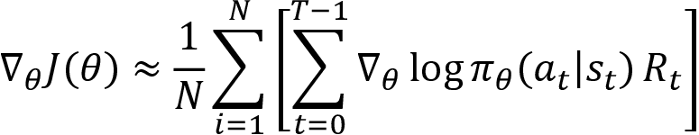
The preceding equation states that the reward-to-go Rt is the sum of rewards of the trajectory starting from the state st. Thus, now we can rewrite our gradient with reward-to-go instead of the return of the trajectory as:
We can simply express the preceding equation as:

After computing the gradient, we update the parameter as:
Now that we have understood what policy gradient with reward-to-go is, in the next section, we will look into the algorithm for more clarity.
Algorithm – Reward-to-go policy gradient
The algorithm of policy gradient with reward-to-go is similar to the REINFORCE method, except now we compute the reward-to-go (return of the trajectory starting from a state st) instead of using the full return of the trajectory, as shown here:
- Initialize the network parameter with random values
- Generate N number of trajectories following the policy
- Compute the return (reward-to-go) Rt
- Compute the gradients:
- Update the network parameter as

- Repeat steps 2 to 5 for several iterations
From the preceding algorithm, we can observe that we are using reward-to-go instead of the return of the trajectory. To get a clear understanding of how the reward-to-go policy gradient works, let's implement it in the next section.
Cart pole balancing with policy gradient
Now, let's learn how to implement the policy gradient algorithm with reward-to-go for the cart pole balancing task.
For a clear understanding of how the policy gradient method works, we use TensorFlow in the non-eager mode by disabling TensorFlow 2 behavior.
First, let's import the necessary libraries:
import tensorflow.compat.v1 as tf
tf.disable_v2_behavior()
import numpy as np
import gym
Create the cart pole environment using gym:
env = gym.make('CartPole-v0')
Get the state shape:
state_shape = env.observation_space.shape[0]
Get the number of actions:
num_actions = env.action_space.n
Computing discounted and normalized reward
Instead of using the rewards directly, we can use the discounted and normalized rewards.
Set the discount factor, ![]() :
:
gamma = 0.95
Let's define a function called discount_and_normalize_rewards for computing the discounted and normalized rewards:
def discount_and_normalize_rewards(episode_rewards):
Initialize an array for storing the discounted rewards:
discounted_rewards = np.zeros_like(episode_rewards)
Compute the discounted reward:
    reward_to_go = 0.0
    for i in reversed(range(len(episode_rewards))):
        reward_to_go = reward_to_go * gamma + episode_rewards[i]
        discounted_rewards[i] = reward_to_go
Normalize and return the reward:
    discounted_rewards -= np.mean(discounted_rewards)
    discounted_rewards /= np.std(discounted_rewards)

    return discounted_rewards
Building the policy network
First, let's define the placeholder for the state:
state_ph = tf.placeholder(tf.float32, [None, state_shape], name="state_ph")
Define the placeholder for the action:
action_ph = tf.placeholder(tf.int32, [None, num_actions], name="action_ph")
Define the placeholder for the discounted reward:
discounted_rewards_ph = tf.placeholder(tf.float32, [None,], name="discounted_rewards")
Define layer 1:
layer1 = tf.layers.dense(state_ph, units=32, activation=tf.nn.relu)
Define layer 2. Note that the number of units in layer 2 is set to the number of actions:
layer2 = tf.layers.dense(layer1, units=num_actions)
Obtain the probability distribution over the action space as an output of the network by applying the softmax function to the result of layer 2:
prob_dist = tf.nn.softmax(layer2)
We learned that we compute gradient as:
After computing the gradient, we update the parameter of the network using gradient ascent:
However, it is a standard convention to perform minimization rather than maximization. So, we can convert the preceding maximization objective into the minimization objective by just adding a negative sign. We can implement this using tf.nn.softmax_cross_entropy_with_logits_v2. Thus, we can define the negative log policy as:
neg_log_policy = tf.nn.softmax_cross_entropy_with_logits_v2(logits = layer2, labels = action_ph)
Now, let's define the loss:
loss = tf.reduce_mean(neg_log_policy * discounted_rewards_ph)
Define the train operation for minimizing the loss using the Adam optimizer:
train = tf.train.AdamOptimizer(0.01).minimize(loss)
Training the network
Now, let's train the network for several iterations. For simplicity, let's just generate one episode in every iteration.
Set the number of iterations:
num_iterations = 1000
Start the TensorFlow session:
with tf.Session() as sess:
Initialize all the TensorFlow variables:
sess.run(tf.global_variables_initializer())
For every iteration:
for i in range(num_iterations):
Initialize an empty list for storing the states, actions, and rewards obtained in the episode:
episode_states, episode_actions, episode_rewards = [],[],[]
Set done to False:
done = False
Initialize the Return:
Return = 0
Initialize the state by resetting the environment:
state = env.reset()
While the episode is not over:
while not done:
Reshape the state:
state = state.reshape([1,4])
Feed the state to the policy network and the network returns the probability distribution over the action space as output, which becomes our stochastic policy ![]() :
:
pi = sess.run(prob_dist, feed_dict={state_ph: state})
Now, we select an action using this stochastic policy:
a = np.random.choice(range(pi.shape[1]), p=pi.ravel())
Perform the selected action:
next_state, reward, done, info = env.step(a)
Render the environment:
env.render()
Update the return:
Return += reward
            action = np.zeros(num_actions)
            action[a] = 1
Store the state, action, and reward in their respective lists:
            episode_states.append(state)
            episode_actions.append(action)
            episode_rewards.append(reward)
Update the state to the next state:
state=next_state
Compute the discounted and normalized reward:
discounted_rewards= discount_and_normalize_rewards(episode_rewards)
Define the feed dictionary:
        feed_dict = {state_ph: np.vstack(np.array(episode_states)),
                     action_ph: np.vstack(np.array(episode_actions)),
                     discounted_rewards_ph: discounted_rewards
                    }
Train the network:
loss_, _ = sess.run([loss, train], feed_dict=feed_dict)
Print the return for every 10 iterations:
        if i%10==0:
            print("Iteration:{}, Return: {}".format(i,Return))
Now that we have learned how to implement the policy gradient algorithm with reward-to-go, in the next section, we will learn another interesting variance reduction technique called policy gradient with baseline.
Policy gradient with baseline
We have learned that we find the optimal policy by using a neural network and we update the parameter of our network using gradient ascent:
Where the value of the gradient is:
Now, to reduce variance, we introduce a new function called a baseline function. Subtracting the baseline b from the return (reward-to-go) Rt reduces the variance, so we can rewrite the gradient as:
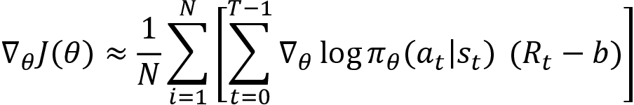
Wait. What is the baseline function? And how does subtracting it from Rt reduce the variance? The purpose of the baseline is to reduce the variance in the return. Thus, if the baseline b is a value that can give us the expected return from the state the agent is in, then subtracting b in every step will reduce the variance in the return.
There are several choices for the baseline functions. We can choose any function as a baseline function but the baseline function should not depend on our network parameter. A simple baseline could be the average return of the sampled trajectories:

Thus, subtracting current return Rt and the average return helps us to reduce variance. As we can see, our baseline function doesn't depend on the network parameter ![]() . So, we can use any function as a baseline function and it should not affect our network parameter
. So, we can use any function as a baseline function and it should not affect our network parameter ![]() .
.
One of the most popular functions of the baseline is the value function. We learned that the value function or the value of a state is the expected return an agent would obtain starting from that state following the policy ![]() . Thus, subtracting the value of a state (the expected return) and the current return Rt can reduce the variance. So, we can rewrite our gradient as:
. Thus, subtracting the value of a state (the expected return) and the current return Rt can reduce the variance. So, we can rewrite our gradient as:

Other than the value function, we can also use different baseline functions such as the Q function, the advantage function, and more. We will learn more about them in the next chapter.
But now the question is how can we learn the baseline function? Say we are using the value function as the baseline function. How can we learn the optimal value function? Just like we are approximating the policy, we can also approximate the value function using another neural network parameterized by ![]() .
.
That is, we use another network for approximating the value function (the value of a state) and we can call this network a value network. Okay, how can we train this value network?
Since the value of the state is a continuous value, we can train the network by minimizing the mean squared error (MSE). The MSE can be defined as the mean squared difference between the actual return Rt and the predicted return  . Thus, the objective function of the value network can be defined as:

We can minimize the error using the gradient descent and update the network parameter as:
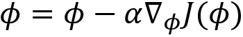
Thus, in the policy gradient with the baseline method, we minimize the variance in the gradient updates by using the baseline function. A baseline function can be any function and it should not depend on the network parameter ![]() . We use the value function as a baseline function, then to approximate the value function we use a different neural network parameterized by
. We use the value function as a baseline function, then to approximate the value function we use a different neural network parameterized by ![]() , and we find the optimal value function by minimizing the MSE.
, and we find the optimal value function by minimizing the MSE.
In a nutshell, in the policy gradient with the baseline function, we use two neural networks:
Policy network parameterized by ![]() : This finds the optimal policy by performing gradient ascent:
: This finds the optimal policy by performing gradient ascent:
Value network parameterized by ![]() : This is used to correct the variance in the gradient update by acting as a baseline, and it finds the optimal value of a state by performing gradient descent:
: This is used to correct the variance in the gradient update by acting as a baseline, and it finds the optimal value of a state by performing gradient descent:
Note that the policy gradient with the baseline function is often referred to as the REINFORCE with baseline method.
Now that we have seen how the policy gradient method with baseline works by using a policy and a value network, in the next section we will look into the algorithm to get more clarity.
Algorithm – REINFORCE with baseline
The algorithm of the policy gradient method with the baseline function (REINFORCE with baseline) is shown here:
- Initialize the policy network parameter
 and value network parameter
- Generate N number of trajectories following the policy

- Compute the return (reward-to-go) Rt
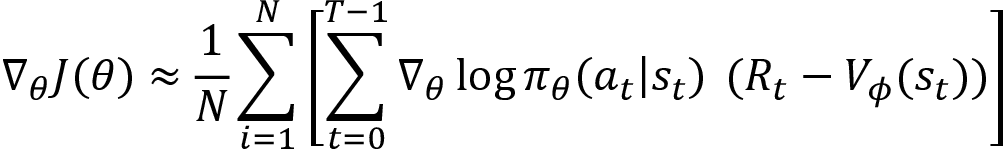
- Compute the policy gradient:

- Update the policy network parameter
 using gradient ascent as
 - Compute the MSE of the value network:
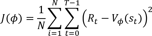
- Compute gradients
 and update the value network parameter using gradient descent as
 - Repeat steps 2 to 7 for several iterations
Summary
We started off the chapter by learning that with value-based methods, we extract the optimal policy from the optimal Q function (Q values). Then we learned that it is difficult to compute the Q function when our action space is continuous. We can discretize the action space; however, discretization is not always desirable, and it leads to the loss of several important features and an action space with a huge set of actions.
So, we resorted to the policy-based method. In the policy-based method, we compute the optimal policy without the Q function. We learned about one of the most popular policy-based methods called the policy gradient, in which we find the optimal policy directly by parameterizing the policy using some parameter ![]() .
.
We also learned that in the policy gradient method, we select actions based on the action probability distribution given by the network, and if we win the episode, that is, if we get a high return, then we assign high probabilities to all the actions in the episode, else we assign low probabilities to all the actions in the episode. Later, we learned how to derive the policy gradient step by step, and then we looked into the algorithm of policy gradient method in more detail.
Moving forward, we learned about the variance reduction methods such as reward-to-go and the policy gradient method with the baseline function. In the policy gradient method with the baseline function, we use two networks called the policy and value network. The role of the policy network is to find the optimal policy, and the role of the value network is to correct the gradient updates in the policy network by estimating the value function.
In the next chapter, we will learn about another interesting set of algorithms called the actor-critic methods.
Questions
Let's evaluate our understanding of the policy gradient method by answering the following questions:
- What is a value-based method?
- Why do we need a policy-based method?
- How does the policy gradient method work?
- How do we compute the gradient in the policy gradient method?
- What is a reward-to-go?
- What is the policy gradient with the baseline function?
- Define the baseline function.
Further reading
For more information about the policy gradient, we can refer to the following paper:
- Policy Gradient Methods for Reinforcement Learning with Function Approximation by Richard S. Sutton et al., https://papers.nips.cc/paper/1713-policy-gradient-methods-for-reinforcement-learning-with-function-approximation.pdf