
4
Monte Carlo Methods
In the previous chapter, we learned how to compute the optimal policy using two interesting dynamic programming methods called value and policy iteration. Dynamic programming is a model-based method and it requires the model dynamics of the environment to compute the value and Q functions in order to find the optimal policy.
But let's suppose we don't have the model dynamics of the environment. In that case, how do we compute the value and Q functions? Here is where we use model-free methods. Model-free methods do not require the model dynamics of the environment to compute the value and Q functions in order to find the optimal policy. One such popular model-free method is the Monte Carlo (MC) method.
We will begin the chapter by understanding what the MC method is, then we will look into two important types of tasks in reinforcement learning called prediction and control tasks. Later, we will learn how the Monte Carlo method is used in reinforcement learning and how it is beneficial compared to the dynamic programming method we learned about in the previous chapter. Moving forward, we will understand what the MC prediction method is and the different types of MC prediction methods. We will also learn how to train an agent to play blackjack with the MC prediction method.
Going ahead, we will learn about the Monte Carlo control method and different types of Monte Carlo control methods. Following this, we will learn how to train an agent to play blackjack with the MC control method.
To summarize, in this chapter, we will learn about the following topics:
- Understanding the Monte Carlo method
- Prediction and control tasks
- The Monte Carlo prediction method
- Playing blackjack with the MC prediction method
- The Monte Carlo control method
- Playing blackjack with the MC control method
Understanding the Monte Carlo method
Before understanding how the Monte Carlo method is useful in reinforcement learning, first, let's understand what the Monte Carlo method is and how it works. The Monte Carlo method is a statistical technique used to find an approximate solution through sampling.
For instance, the Monte Carlo method approximates the expectation of a random variable by sampling, and when the sample size is greater, the approximation will be better. Let's suppose we have a random variable X and say we need to compute the expected value of X; that is E(X), then we can compute it by taking the sum of the values of X multiplied by their respective probabilities as follows:

But instead of computing the expectation like this, can we approximate it with the Monte Carlo method? Yes! We can estimate the expected value of X by just sampling the values of X for some N times and compute the average value of X as the expected value of X as follows:
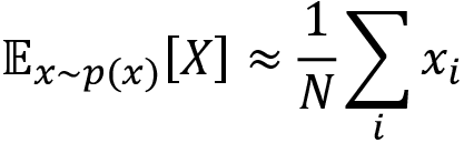
When N is larger our approximation will be better. Thus, with the Monte Carlo method, we can approximate the solution through sampling and our approximation will be better when the sample size is large.
In the upcoming sections, we will learn how exactly the Monte Carlo method is used in reinforcement learning.
Prediction and control tasks
In reinforcement learning, we perform two important tasks, and they are:
- The prediction task
- The control task
Prediction task
In the prediction task, a policy ![]() is given as an input and we try to predict the value function or Q function using the given policy. But what is the use of doing this? Our goal is to evaluate the given policy. That is, we need to determine whether the given policy is good or bad. How can we determine that? If the agent obtains a good return using the given policy then we can say that our policy is good. Thus, to evaluate the given policy, we need to understand what the return the agent would obtain if it uses the given policy. To obtain the return, we predict the value function or Q function using the given policy.
is given as an input and we try to predict the value function or Q function using the given policy. But what is the use of doing this? Our goal is to evaluate the given policy. That is, we need to determine whether the given policy is good or bad. How can we determine that? If the agent obtains a good return using the given policy then we can say that our policy is good. Thus, to evaluate the given policy, we need to understand what the return the agent would obtain if it uses the given policy. To obtain the return, we predict the value function or Q function using the given policy.
That is, we learned that the value function or value of a state denotes the expected return an agent would obtain starting from that state following some policy ![]() . Thus, by predicting the value function using the given policy
. Thus, by predicting the value function using the given policy ![]() , we can understand what the expected return the agent would obtain in each state if it uses the given policy
, we can understand what the expected return the agent would obtain in each state if it uses the given policy ![]() . If the return is good then we can say that the given policy is good.
. If the return is good then we can say that the given policy is good.
Similarly, we learned that the Q function or Q value denotes the expected return the agent would obtain starting from the state s and an action a following the policy ![]() . Thus, predicting the Q function using the given policy
. Thus, predicting the Q function using the given policy ![]() , we can understand what the expected return the agent would obtain in each state-action pair if it uses the given policy. If the return is good then we can say that the given policy is good.
, we can understand what the expected return the agent would obtain in each state-action pair if it uses the given policy. If the return is good then we can say that the given policy is good.
Thus, we can evaluate the given policy ![]() by computing the value and Q functions.
by computing the value and Q functions.
Note that, in the prediction task, we don't make any change to the given input policy. We keep the given policy as fixed and predict the value function or Q function using the given policy and obtain the expected return. Based on the expected return, we evaluate the given policy.
Control task
Unlike the prediction task, in the control task, we will not be given any policy as an input. In the control task, our goal is to find the optimal policy. So, we will start off by initializing a random policy and we try to find the optimal policy iteratively. That is, we try to find an optimal policy that gives the maximum return.
Thus, in a nutshell, in the prediction task, we evaluate the given input policy by predicting the value function or Q function, which helps us to understand the expected return an agent would get if it uses the given policy, while in the control task our goal is to find the optimal policy and we will not be given any policy as input; so we will start off by initializing a random policy and we try to find the optimal policy iteratively.
Now that we have understood what prediction and control tasks are, in the next section, we will learn how to use the Monte Carlo method for performing the prediction and control tasks.
Monte Carlo prediction
In this section, we will learn how to use the Monte Carlo method to perform the prediction task. We have learned that in the prediction task, we will be given a policy and we predict the value function or Q function using the given policy to evaluate it. First, we will learn how to predict the value function using the given policy with the Monte Carlo method. Later, we will look into predicting the Q function using the given policy. Alright, let's get started with the section.
Why do we need the Monte Carlo method for predicting the value function of the given policy? Why can't we predict the value function using the dynamic programming methods we learned about in the previous chapter? We learned that in order to compute the value function using the dynamic programming method, we need to know the model dynamics (transition probability), and when we don't know the model dynamics, we use the model-free methods.
The Monte Carlo method is a model-free method, meaning that it doesn't require the model dynamics to compute the value function.
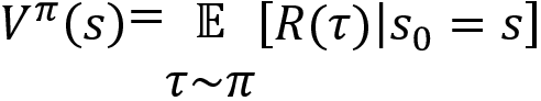
First, let's recap the definition of the value function. The value function or the value of the state s can be defined as the expected return the agent would obtain starting from the state s and following the policy ![]() . It can be expressed as:
. It can be expressed as:
Okay, how can we estimate the value of the state (value function) using the Monte Carlo method? At the beginning of the chapter, we learned that the Monte Carlo method approximates the expected value of a random variable by sampling, and when the sample size is greater, the approximation will be better. Can we leverage this concept of the Monte Carlo method to predict the value of a state? Yes!
In order to approximate the value of the state using the Monte Carlo method, we sample episodes (trajectories) following the given policy ![]() for some N times and then we compute the value of the state as the average return of a state across the sampled episodes, and it can be expressed as:
for some N times and then we compute the value of the state as the average return of a state across the sampled episodes, and it can be expressed as:
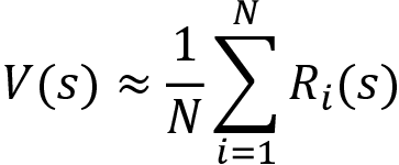
From the preceding equation, we can understand that the value of a state s can be approximated by computing the average return of the state s across some N episodes. Our approximation will be better when N is higher.
In a nutshell, in the Monte Carlo prediction method, we approximate the value of a state by taking the average return of a state across N episodes instead of taking the expected return.
Okay, let's get a better understanding of how the Monte Carlo method estimates the value of a state (value function) with an example. Let's take our favorite grid world environment we covered in Chapter 1, Fundamentals of Reinforcement Learning, as shown in Figure 4.1. Our goal is to reach the state I from the state A without visiting the shaded states, and the agent receives +1 reward when it visits the unshaded states and -1 reward when it visits the shaded states:
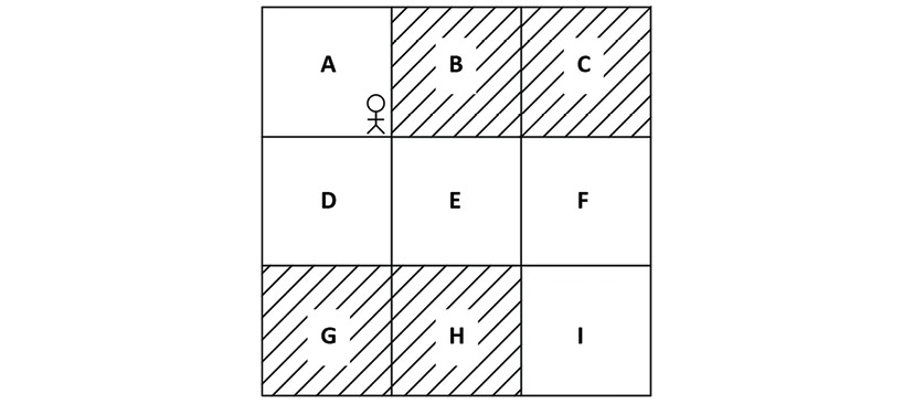
Figure 4.1: Grid world environment
Let's say we have a stochastic policy ![]() . Let's suppose, in state A, our stochastic policy
. Let's suppose, in state A, our stochastic policy ![]() selects action down 80% of time and action right 20% of the time, and it selects action right in states D and E and action down in states B and F 100% of the time.
selects action down 80% of time and action right 20% of the time, and it selects action right in states D and E and action down in states B and F 100% of the time.
First, we generate an episode ![]() using our given stochastic policy
using our given stochastic policy ![]() as Figure 4.2 shows:
as Figure 4.2 shows:

Figure 4.2: Episode ![]()
For a better understanding, let's focus only on state A. Let's now compute the return of state A. The return of a state is the sum of the rewards of the trajectory starting from that state. Thus, the return of state A is computed as R1(A) = 1+1+1+1 = 4 where the subscript 1 in R1 indicates the return from episode 1.
Say we generate another episode ![]() using the same given stochastic policy
using the same given stochastic policy ![]() as Figure 4.3 shows:
as Figure 4.3 shows:

Figure 4.3: Episode ![]()
Let's now compute the return of state A. The return of state A is R2(A) = -1+1+1+1 = 2.
Say we generate another episode ![]() using the same given stochastic policy
using the same given stochastic policy ![]() as Figure 4.4 shows:
as Figure 4.4 shows:

Figure 4.4: Episode ![]()
Let's now compute the return of state A. The return of state A is R3(A) = 1+1+1+1 = 4.
Thus, we generated three episodes and computed the return of state A in all three episodes. Now, how can we compute the value of the state A? We learned that in the Monte Carlo method, the value of a state can be approximated by computing the average return of the state across some N episodes (trajectories):
We need to compute the value of state A, so we can compute it by just taking the average return of the state A across the N episodes as:

We generated three episodes, thus:


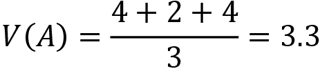
Thus, the value of state A is 3.3. Similarly, we can compute the value of all other states by just taking the average return of the state across the three episodes.
For easier understanding, in the preceding example, we only generated three episodes. In order to find a better and more accurate estimate of the value of the state, we should generate many episodes (not just three) and compute the average return of the state as the value of the state.
Thus, in the Monte Carlo prediction method, to predict the value of a state (value function) using the given input policy ![]() , we generate some N episodes using the given policy and then we compute the value of a state as the average return of the state across these N episodes.
, we generate some N episodes using the given policy and then we compute the value of a state as the average return of the state across these N episodes.
Note that while computing the return of the state, we can also include the discount factor and compute the discounted return, but for simplicity let's not include the discount factor.
Now, that we have a basic understanding of how the Monte Carlo prediction method predicts the value function of the given policy, let's look into more detail by understanding the algorithm of the Monte Carlo prediction method in the next section.
MC prediction algorithm
The Monte Carlo prediction algorithm is given as follows:
- Let total_return(s) be the sum of return of a state across several episodes and N(s) be the counter, that is, the number of times a state is visited across several episodes. Initialize total_return(s) and N(s) as zero for all the states. The policy
 is given as input.
 - For M number of iterations:
- Generate an episode using the policy

- Store all the rewards obtained in the episode in the list called rewards
- For each step t in the episode:
- Compute the return of state st as R(st) = sum(rewards[t:])
- Update the total return of state st as total_returns(st) = total_return(st) + R(st)
- Update the counter as N(st) = N(st) + 1
- Generate an episode using the policy
- Compute the value of a state by just taking the average, that is:

The preceding algorithm implies that the value of the state is just the average return of the state across several episodes.
To get a better understanding of how exactly the preceding algorithm works, let's take a simple example and compute the value of each state manually. Say we need to compute the value of three states s0, s1, and s2. We know that we obtain a reward when we transition from one state to another. Thus, the reward for the final state will be 0 as we don't make any transitions from the final state. Hence, the value of the final state s2 will be zero. Now, we need to find the value of two states s0 and s1.
The upcoming sections are explained with manual calculations, for a better understanding, follow along with a pen and paper.
Step 1:
Initialize the total_returns(s) and N(s) for all the states to zero as Table 4.1 shows:

Table 4.1: Initial values
Say we are given a stochastic policy ![]() ; in state s0 our stochastic policy selects the action 0 for 50% of the time and action 1 for 50% of the time, and it selects action 1 in state s1 for 100% of the time.
; in state s0 our stochastic policy selects the action 0 for 50% of the time and action 1 for 50% of the time, and it selects action 1 in state s1 for 100% of the time.
Step 2: Iteration 1:
Generate an episode using the given input policy ![]() , as Figure 4.5 shows:
, as Figure 4.5 shows:
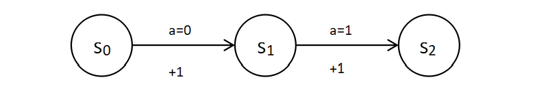
Figure 4.5: Generating an episode using the given policy ![]()
Store all rewards obtained in the episode in the list called rewards. Thus, rewards = [1, 1].
First, we compute the return of the state s0 (sum of rewards from s0):
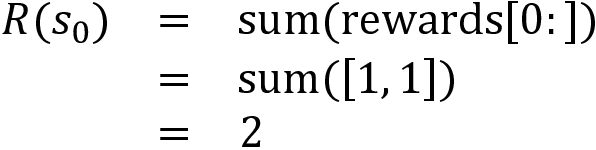
Update the total return of the state s0 in our table as:

Update the number of times the state s0 is visited in our table as:

Now, let's compute the return of the state s1 (sum of rewards from s1):
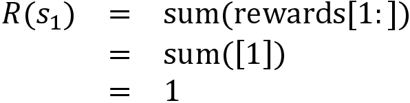
Update the total return of the state s1 in our table as:

Update the number of times the state s1 is visited in our table as:

Our updated table, after iteration 1, is as follows:

Table 4.2: Updated table after the first iteration
Iteration 2:
Say we generate another episode using the same given policy ![]() as Figure 4.6 shows:
as Figure 4.6 shows:
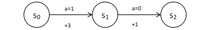
Figure 4.6: Generating an episode using the given policy ![]()
Store all rewards obtained in the episode in the list called rewards. Thus, rewards = [3, 1].
First, we compute the return of the state s0 (sum of rewards from s0):

Update the total return of the state s0 in our table as:

Update the number of times the state s0 is visited in our table as:

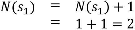
Now, let's compute the return of the state s1 (sum of rewards from s1):
Update the return of the state s1 in our table as:

Update the number of times the state is visited:
Our updated table after the second iteration is as follows:

Table 4.3: Updated table after the second iteration
Since we are computing manually, for simplicity, let's stop at two iterations; that is, we just generate only two episodes.
Step 3:
Now, we can compute the value of the state as:

Thus:
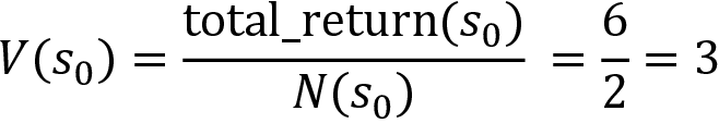

Thus, we computed the value of the state by just taking the average return across multiple episodes. Note that in the preceding example, for our manual calculation, we just generated two episodes, but for a better estimation of the value of the state, we generate several episodes and then we compute the average return across those episodes (not just 2).
Types of MC prediction
We just learned how the Monte Carlo prediction algorithm works. We can categorize the Monte Carlo prediction algorithm into two types:
- First-visit Monte Carlo
- Every-visit Monte Carlo
First-visit Monte Carlo
We learned that in the MC prediction method, we estimate the value of the state by just taking the average return of the state across multiple episodes. We know that in each episode a state can be visited multiple times. In the first-visit Monte Carlo method, if the same state is visited again in the same episode, we don't compute the return for that state again. For example, consider a case where an agent is playing snakes and ladders. If the agent lands on a snake, then there is a good chance that the agent will return to a state that it had visited earlier. So, when the agent revisits the same state, we don't compute the return for that state for the second time.
The following shows the algorithm of first-visit MC; as the point in bold says, we compute the return for the state st only if it is occurring for the first time in the episode:
- Let total_return(s) be the sum of return of a state across several episodes and N(s) be the counter, that is, the number of times a state is visited across several episodes. Initialize total_return(s) and N(s) as zero for all the states. The policy
 is given as input
 - For M number of iterations:
- Generate an episode using the policy

- Store all the rewards obtained in the episode in the list called rewards
- For each step t in the episode:
If the state st is occurring for the first time in the episode:
- Compute the return of the state st as R(st) = sum(rewards[t:])
- Update the total return of the state st as total_return(st) = total_return(st) + R(st)
- Update the counter as N(st) = N(st) + 1
- Generate an episode using the policy
- Compute the value of a state by just taking the average, that is:

Every-visit Monte Carlo
As you might have guessed, every-visit Monte Carlo is just the opposite of first-visit Monte Carlo. Here, we compute the return every time a state is visited in the episode. The algorithm of every-visit Monte Carlo is the same as the one we saw earlier at the beginning of this section and it is as follows:
- Let total_return(s) be the sum of the return of a state across several episodes and N(s) be the counter, that is, the number of times a state is visited across several episodes. Initialize total_return(s) and N(s) as zero for all the states. The policy
 is given as input
 - For M number of iterations:
- Generate an episode using the policy
- Store all the rewards obtained in the episode in the list called rewards
- For each step t in the episode:
- Compute the return of the state st as R(st) = sum(rewards[t:])
- Update the total return of the state st as total_return(st) = total_return(st) + R(st)
- Update the counter as N(st) = N(st) + 1
- Generate an episode using the policy
- Compute the value of a state by just taking the average, that is:
Remember that the only difference between the first-visit MC and every-visit MC methods is that in the first-visit MC method, we compute the return for a state only for its first time of occurrence in the episode but in the every-visit MC method, the return of the state is computed every time the state is visited in an episode. We can choose between first-visit MC and every-visit MC based on the problem that we are trying to solve.
Now that we have understood how the Monte Carlo prediction method predicts the value function of the given policy, in the next section, we will learn how to implement the Monte Carlo prediction method.
Implementing the Monte Carlo prediction method
If you love playing card games then this section is definitely going to be interesting for you. In this section, we will learn how to play blackjack with the Monte Carlo prediction method. Before diving in, let's understand how the blackjack game works and its rules.
Understanding the blackjack game
Blackjack, also known as 21, is one of the most popular card games. The game consists of a player and a dealer. The goal of the player is to have the value of the sum of all their cards be 21 or a larger value than the sum of the dealer's cards while not exceeding 21. If one of these criteria is met then the player wins the game; else the dealer wins the game. Let's understand this in more detail.
The values of the cards Jack (J), King (K), and Queen (Q) will be considered as 10. The value of the Ace (A) can be 1 or 11, depending on the player's choice. That is, the player can decide whether the value of an Ace should be 1 or 11 during the game. The value of the rest of the cards (2 to 10) is just their face value. For instance, the value of the card 2 will be 2, the value of the card 3 will be 3, and so on.
We learned that the game consists of a player and a dealer. There can be many players at a time but only one dealer. All the players compete with the dealer and not with other players. Let's consider a case where there is only one player and a dealer. Let's understand blackjack by playing the game along with different cases. Let's suppose we are the player and we are competing with the dealer.
Case 1: When the player wins the game
Initially, a player is given two cards. Both of these cards are face up, that is, both of the player's cards are visible to the dealer. Similarly, the dealer is also given two cards. But one of the dealer's cards is face up, and the other is face down. That is, the dealer shows only one of their cards.
As we can see in Figure 4.7, the player has two cards (both face up) and the dealer also has two cards (only one face up):
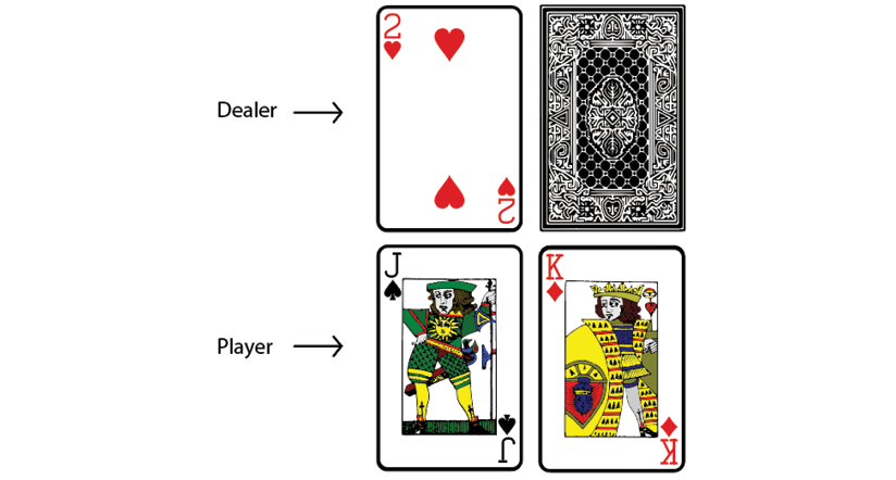
Figure 4.7: The player has 20, and the dealer has 2 with one card face down
Now, the player performs either of the two actions, which are Hit and Stand. If we (the player) perform the action hit, then we get one more card. If we perform stand, then it implies that we don't need any more cards and tells the dealer to show all their cards. Whoever has a sum of cards value equal to 21 or a larger value than the other player but not exceeding 21 wins the game.
We learned that the value of J, K, and Q is 10. As shown in Figure 4.7, we have cards J and K, which sums to 20 (10+10). Thus, the total value our cards is already a large number and it didn't exceed 21. So we stand, and this action tells the dealer to show their cards. As we can observe in Figure 4.8, the dealer has now shown all their cards and the total value of the dealer's cards is 12 and the total value of our (the player's) cards is 20, which is larger and also didn't exceed 21, so we win the game.

Figure 4.8: The player wins!
Case 2: When the player loses the game
Figure 4.9 shows we have two cards and the dealer also has two cards and only one of the dealer's card is visible to us:

Figure 4.9: The player has 13, and the dealer has 7 with one card face down
Now, we have to decide whether we should (perform the action) hit or stand. Figure 4.9 shows we have two cards, K and 3, which sums to 13 (10+3). Let's be a little optimistic and hope that the total value of the dealer's cards will not be greater than ours. So we stand, and this action tells the dealer to show their cards. As we can observe in Figure 4.10, the sum of the dealer's card is 17, but ours is only 13, so we lose the game. That is, the dealer has got a larger value than us, and it did not exceed 21, so the dealer wins the game, and we lose:

Figure 4.10: The dealer wins!
Case 3: When the player goes bust
Figure 4.11 shows we have two cards and the dealer also has two cards but only one of the dealer's cards is visible to us:

Figure 4.11: The player has 8, and the dealer has 10 with one card face down
Now, we have to decide whether we should (perform the action) hit or stand. We learned that the goal of the game is to have a sum of cards value of 21, or a larger value than the dealer while not exceeding 21. Right now, the total value of our cards is just 3+5 = 8. Thus, we (perform the action) hit so that we can make our sum value larger. After we hit, we receive a new card as shown in Figure 4.12:

Figure 4.12: The player has 18, and the dealer has 10 with one card face down
As we can observe, we got a new card. Now, the total value of our cards is 3+5+10 = 18. Again, we need to decide whether we should (perform the action) hit or stand. Let's be a little greedy and (perform the action) hit so that we can make our sum value a little larger. As shown in Figure 4.13, we hit and received one more card but now the total value of our cards becomes 3+5+10+10 = 28, which exceeds 21, and this is called a bust and we lose the game:
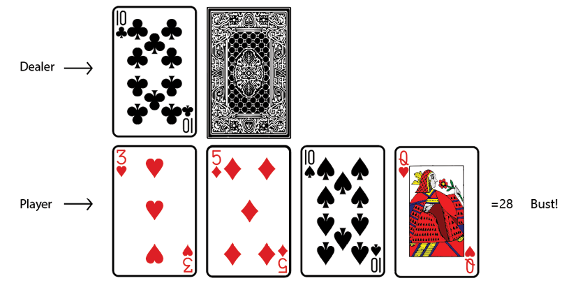
Figure 4.13: The player goes bust!
Case 4: Useable Ace
We learned that the value of the Ace can be either 1 or 11, and the player can decide the value of the ace during the game. Let's learn how this works. As Figure 4.14 shows, we have been given two cards and the dealer also has two cards and only one of the dealer's cards is face up:

Figure 4.14: The player has 10, and the dealer has 5 with one card face down
As we can see, the total value of our cards is 5+5 = 10. Thus, we hit so that we can make our sum value larger. As Figure 4.15 shows, after performing the hit action we received a new card, which is an Ace. Now, we can decide the value of the Ace to be either 1 or 11. If we consider the value of Ace to be 1, then the total value of our cards will be 5+5+1 = 11. But if we consider the value of the Ace to be 11, then the total value of our cards will be 5+5+11 = 21. In this case, we consider the value of our Ace to be 11 so that our sum value becomes 21.
Thus, we set the value of the Ace to be 11 and win the game, and in this case, the Ace is called the usable Ace since it helped us to win the game:
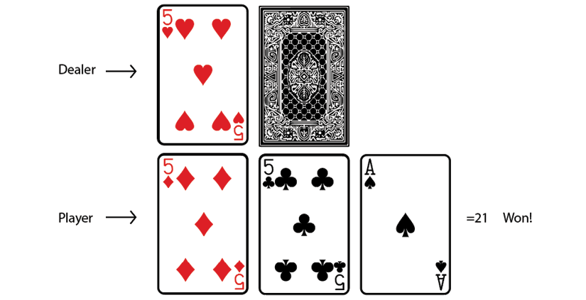
Figure 4.15: The player uses the Ace as 11 and wins the game
Case 5: Non-usable Ace
Figure 4.16 shows we have two cards and the dealer has two cards with one face up:
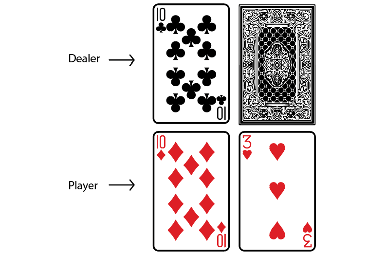
Figure 4.16: The player has 13, and the dealer has 10 with one card face down
As we can observe, the total value of our cards is 13 (10+3). We (perform the action) hit so that we can make our sum value a little larger:
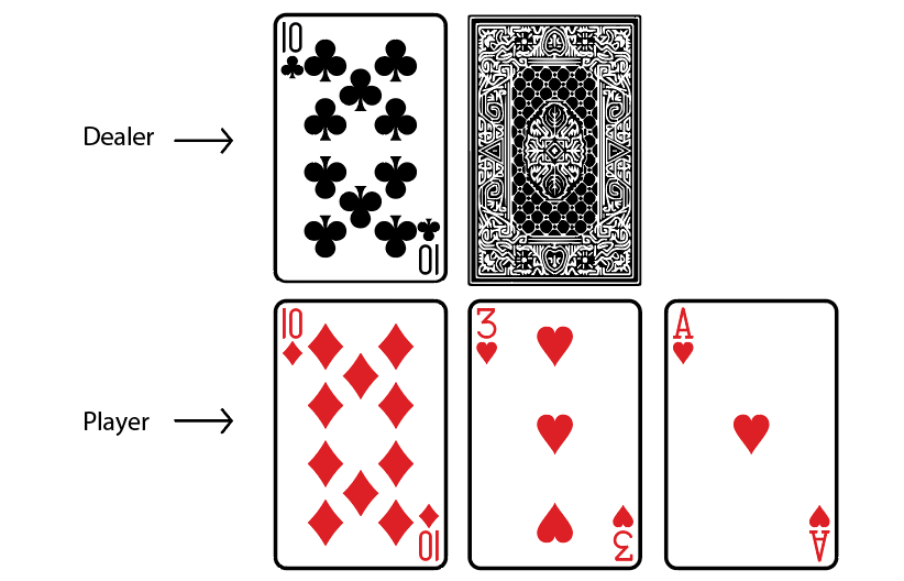
Figure 4.17: The player has to use the Ace as a 1 else they go bust
As Figure 4.17 shows, we hit and received a new card, which is an Ace. Now we can decide the value of Ace to be 1 or 11. If we choose 11, then our sum value becomes 10+3+11 = 23. As we can observe, when we set our ace to 11, then our sum value exceeds 21, and we lose the game. Thus, instead of choosing Ace = 11, we set the Ace value to be 1; so our sum value becomes 10+3+1 = 14.
Again, we need to decide whether we should (perform the action) hit or stand. Let's say we stand hoping that the dealer sum value will be lower than ours. As Figure 4.18 shows, after performing the stand action, both of the dealer's cards are shown, and the sum of the dealer's card is 20, but ours is just 14, and so we lose the game, and in this case, the Ace is called a non-usable Ace since it did not help us to win the game.
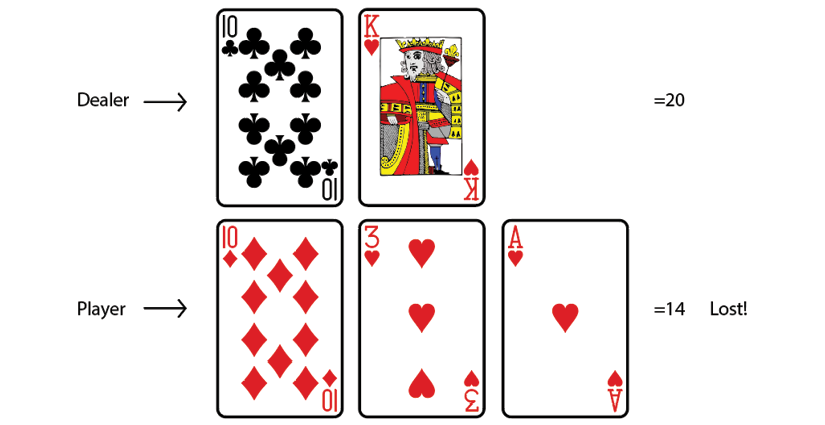
Figure 4.18: The player has 14, and the dealer has 20 and wins
Case 6: When the game is a draw
If both the player and the dealer's sum of cards value is the same, say 20, then the game is called a draw.
Now that we have understood how to play blackjack, let's implement the Monte Carlo prediction method in the blackjack game. But before going ahead, first, let's learn how the blackjack environment is designed in Gym.
The blackjack environment in the Gym library
import gym
The environment id of blackjack is Blackjack-v0. So, we can create the blackjack game using the make function as shown as follows:
env = gym.make('Blackjack-v0')
Now, let's look at the state of the blackjack environment; we can just reset our environment and look at the initial state:
print(env.reset())
Note that every time we run the preceding code, we might get a different result, as the initial state is randomly initialized. The preceding code will print something like this:
(15, 9, True)
As we can observe, our state is represented as a tuple, but what does this mean? We learned that in the blackjack game, we will be given two cards and we also get to see one of the dealer's cards. Thus, 15 implies that the value of the sum of our cards, 9 implies the face value of one of the dealer's cards, True implies that we have a usable ace, and it will be False if we don't have a usable ace.
Thus, in the blackjack environment the state is represented as a tuple consisting of three values:
- The value of the sum of our cards
- The face value of one of the dealer's card
- Boolean value—
Trueif we have a useable ace andFalseif we don't have a useable ace
Let's look at the action space of our blackjack environment:
print(env.action_space)
The preceding code will print:
Discrete(2)
As we can observe, it implies that we have two actions in our action space, which are 0 and 1:
- The action stand is represented by 0
- The action hit is represented by 1
Okay, what about the reward? The reward will be assigned as follows:
- +1.0 reward if we win the game
- -1.0 reward if we lose the game
- 0 reward if the game is a draw
Now that we have understood how the blackjack environment is designed in Gym, let's start implementing the MC prediction method in the blackjack game. First, we will look at every-visit MC and then we will learn how to implement first-visit MC prediction.
Every-visit MC prediction with the blackjack game
To understand this section clearly, you should recap the every-visit Monte Carlo method we learned earlier. Let's now understand how to implement every-visit MC prediction with the blackjack game step by step:
Import the necessary libraries:
import gym
import pandas as pd
from collections import defaultdict
Create a blackjack environment:
env = gym.make('Blackjack-v0')
Defining a policy
We learned that in the prediction method, we will be given an input policy and we predict the value function of the given input policy. So, now, we first define a policy function that acts as an input policy. That is, we define the input policy whose value function will be predicted in the upcoming steps.
As shown in the following code, our policy function takes the state as an input and if the state[0], the sum of our cards, value, is greater than 19, then it will return action 0 (stand), else it will return action 1 (hit):
def policy(state):
    return 0 if state[0] > 19 else 1
We defined an optimal policy: it makes more sense to perform an action 0 (stand) when our sum value is already greater than 19. That is, when the sum value is greater than 19 we don't have to perform a 1 (hit) action and receive a new card, which may cause us to lose the game or bust.
For example, let's generate an initial state by resetting the environment as shown as follows:
state = env.reset()
print(state)
Suppose the preceding code prints the following:
(20, 5, False)
As we can notice, state[0] = 20; that is, the value of the sum of our cards is 20, so in this case, our policy will return the action 0 (stand) as the following shows:
print(policy(state))
The preceding code will print:
0
Now that we have defined the policy, in the next sections, we will predict the value function (state values) of this policy.
Generating an episode
Next, we generate an episode using the given policy, so we define a function called generate_episode, which takes the policy as an input and generates the episode using the given policy.
First, let's set the number of time steps:
num_timesteps = 100
For a clear understanding, let's look into the function line by line:
def generate_episode(policy):
Let's define a list called episode for storing the episode:
episode = []
Initialize the state by resetting the environment:
state = env.reset()
Then for each time step:
for t in range(num_timesteps):
Select the action according to the given policy:
action = policy(state)
Perform the action and store the next state information:
next_state, reward, done, info = env.step(action)
Store the state, action, and reward into our episode list:
episode.append((state, action, reward))
If the next state is a final state then break the loop, else update the next state to the current state:
        if done:
            break

        state = next_state
    return episode
Let's take a look at what the output of our generate_episode function looks like. Note that we generate an episode using the policy we defined earlier:
print(generate_episode(policy))
The preceding code will print something like the following:
[((10, 2, False), 1, 0), ((20, 2, False), 0, 1.0)]
As we can observe our output is in the form of [(state, action, reward)]. As shown previously, we have two states in our episode. We performed action 1 (hit) in the state (10, 2, False) and received a 0 reward, and we performed action 0 (stand) in the state (20, 2, False) and received a reward of 1.0.
Now that we have learned how to generate an episode using the given policy, next, we will look at how to compute the value of the state (value function) using the every-visit MC method.
Computing the value function
We learned that in order to predict the value function, we generate several episodes using the given policy and compute the value of the state as an average return across several episodes. Let's see how to implement that.
First, we define the total_return and N as a dictionary for storing the total return and the number of times the state is visited across episodes respectively:
total_return = defaultdict(float)
N = defaultdict(int)
Set the number of iterations, that is, the number of episodes, we want to generate:
num_iterations = 500000
Then, for every iteration:
for i in range(num_iterations):
Generate the episode using the given policy; that is, generate an episode using the policy function we defined earlier:
episode = generate_episode(policy)
Store all the states, actions, and rewards obtained from the episode:
states, actions, rewards = zip(*episode)
Then, for each step in the episode:
for t, state in enumerate(states):
Compute the return R of the state as the sum of rewards, R(st) = sum(rewards[t:]):
R = (sum(rewards[t:]))
Update the total_return of the state as total_return(st) = total_return(st) + R(st):
total_return[state] = total_return[state] + R
Update the number of times the state is visited in the episode as N(st) = N(st) + 1:
N[state] = N[state] + 1
After computing the total_return and N we can just convert them into a pandas data frame for a better understanding. Note that this is just to give a clear understanding of the algorithm; we don't necessarily have to convert to the pandas data frame, we can also implement this efficiently just by using the dictionary.
Convert the total_returns dictionary into a data frame:
total_return = pd.DataFrame(total_return.items(),columns=['state', 'total_return'])
Convert the counter N dictionary into a data frame:
N = pd.DataFrame(N.items(),columns=['state', 'N'])
Merge the two data frames on states:
df = pd.merge(total_return, N, on="state")
Look at the first few rows of the data frame:
df.head(10)
The preceding code will display the following. As we can observe, we have the total return and the number of times the state is visited:
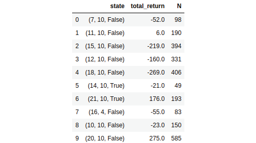
Figure 4.19: The total return and the number of times a state has been visited
Next, we can compute the value of the state as the average return:
Thus, we can write:
df['value'] = df['total_return']/df['N']
Let's look at the first few rows of the data frame:
df.head(10)
The preceding code will display something like this:
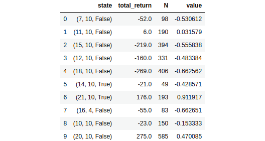
Figure 4.20: The value is calculated as the average of the return of each state
As we can observe, we now have the value of the state, which is just the average of a return of the state across several episodes. Thus, we have successfully predicted the value function of the given policy using the every-visit MC method.
Okay, let's check the value of some states and understand how accurately our value function is estimated according to the given policy. Recall that when we started off, to generate episodes, we used the optimal policy, which selects the action 0 (stand) when the sum value is greater than 19 and the action 1 (hit) when the sum value is lower than 19.
Let's evaluate the value of the state (21,9,False), as we can observe, the value of the sum of our cards is already 21 and so this is a good state and should have a high value. Let's see what our estimated value of the state is:
df[df['state']==(21,9,False)]['value'].values
The preceding will print something like this:
array([1.0])
As we can observe, the value of the state is high.
Now, let's check the value of the state (5,8,False). As we can notice, the value of the sum of our cards is just 5 and even the one dealer's single card has a high value, 8; in this case, the value of the state should be lower. Let's see what our estimated value of the state is:
df[df['state']==(5,8,False)]['value'].values
The preceding code will print something like this:
array([-1.0])
As we can notice, the value of the state is lower.
Thus, we learned how to predict the value function of the given policy using the every-visit MC prediction method. In the next section, we will look at how to compute the value of the state using the first-visit MC method.
First-visit MC prediction with the blackjack game
Predicting the value function using the first-visit MC method is exactly the same as how we predicted the value function using the every-visit MC method, except that here we compute the return of a state only for its first time of occurrence in the episode. The code for first-visit MC is the same as what we have seen in every-visit MC except here, we compute the return only for its first time of occurrence as shown in the following highlighted code:
for i in range(num_iterations):

    episode = generate_episode(env,policy)
    states, actions, rewards = zip(*episode)
    for t, state in enumerate(states):
        if state not in states[0:t]:
            R = (sum(rewards[t:]))
            total_return[state] = total_return[state] + R
            N[state] = N[state] + 1
You can obtain the complete code from the GitHub repo of the book and you will get results similar to what we saw in the every-visit MC section.
Thus, we learned how to predict the value function of the given policy using the first-visit and every-visit MC methods.
Incremental mean updates
In both first-visit MC and every-visit MC, we estimate the value of a state as an average (arithmetic mean) return of the state across several episodes as shown as follows:
Instead of using the arithmetic mean to approximate the value of the state, we can also use the incremental mean, and it is expressed as:

But why do we need incremental mean? Consider our environment as non-stationary. In that case, we don't have to take the return of the state from all the episodes and compute the average. As the environment is non-stationary we can ignore returns from earlier episodes and use only the returns from the latest episodes for computing the average. Thus, we can compute the value of the state using the incremental mean as shown as follows:

Where  and Rt is the return of the state st.
MC prediction (Q function)
So far, we have learned how to predict the value function of the given policy using the Monte Carlo method. In this section, we will see how to predict the Q function of the given policy using the Monte Carlo method.
Predicting the Q function of the given policy using the MC method is exactly the same as how we predicted the value function in the previous section except that here we use the return of the state-action pair, whereas in the case of the value function we used the return of the state. That is, just like we approximated the value of a state (value function) by computing the average return of the state across several episodes, we can also approximate the value of a state-action pair (Q function) by computing the average return of the state-action pair across several episodes.
Thus, we generate several episodes using the given policy ![]() , then, we calculate the total_return(s, a), the sum of the return of the state-action pair across several episodes, and also we calculate N(s, a), the number of times the state-action pair is visited across several episodes. Then we compute the Q function or Q value as the average return of the state-action pair as shown as follows:
, then, we calculate the total_return(s, a), the sum of the return of the state-action pair across several episodes, and also we calculate N(s, a), the number of times the state-action pair is visited across several episodes. Then we compute the Q function or Q value as the average return of the state-action pair as shown as follows:

For instance, let consider a small example. Say we have two states s0 and s1 and we have two possible actions 0 and 1. Now, we compute total_return(s, a) and N(s, a). Let's say our table after computation looks like Table 4.4:
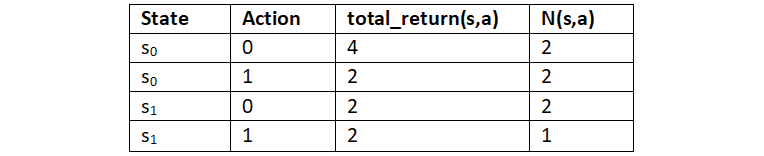
Table 4.4: The result of two actions in two states
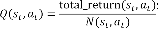
Once we have this, we can compute the Q value by just taking the average, that is:
Thus, we can compute the Q value for all state-action pairs as:


The algorithm for predicting the Q function using the Monte Carlo method is as follows. As we can see, it is exactly the same as how we predicted the value function using the return of the state except that here we predict the Q function using the return of a state-action pair:
- Let total_return(s, a) be the sum of the return of a state-action pair across several episodes and N(s, a) be the number of times a state-action pair is visited across several episodes. Initialize total_return(s, a) and N(s, a) for all state-action pairs to zero. The policy
 is given as input
 - For M number of iterations:
- Generate an episode using policy
- Store all rewards obtained in the episode in the list called rewards
- For each step t in the episode:
- Compute return for the state-action pair, R(st, at) = sum(rewards[t:])
- Update the total return of the state-action pair, total_return(st, at) = total_return(st, at) + R(st, at)
- Update the counter as N(st, at) = N(st, at) + 1
- Generate an episode using policy
- Compute the Q function (Q value) by just taking the average, that is:
Recall that in the MC prediction of the value function, we learned two types of MC—first-visit MC and every-visit MC. In first-visit MC, we compute the return of the state only for the first time the state is visited in the episode and in every-visit MC we compute the return of the state every time the state is visited in the episode.
Similarly, in the MC prediction of the Q function, we have two types of MC—first-visit MC and every-visit MC. In first-visit MC, we compute the return of the state-action pair only for the first time the state-action pair is visited in the episode and in every-visit MC we compute the return of the state-action pair every time the state-action pair is visited in the episode.
As mentioned in the previous section, instead of using the arithmetic mean, we can also use the incremental mean. We learned that the value of a state can be computed using the incremental mean as:
Similarly, we can also compute the Q value using the incremental mean as shown as follows:

Now that we have learned how to perform the prediction task using the Monte Carlo method, in the next section, we will learn how to perform the control task using the Monte Carlo method.
Monte Carlo control
In the control task, our goal is to find the optimal policy. Unlike the prediction task, here, we will not be given any policy as an input. So, we will begin by initializing a random policy, and then we try to find the optimal policy iteratively. That is, we try to find an optimal policy that gives the maximum return. In this section, we will learn how to perform the control task to find the optimal policy using the Monte Carlo method.
Okay, we learned that in the control task our goal is to find the optimal policy. First, how can we compute a policy? We learned that the policy can be extracted from the Q function. That is, if we have a Q function, then we can extract policy by selecting an action in each state that has the maximum Q value as the following shows:

So, to compute a policy, we need to compute the Q function. But how can we compute the Q function? We can compute the Q function similarly to what we learned in the MC prediction method. That is, in the MC prediction method, we learned that when given a policy, we can generate several episodes using that policy and compute the Q function (Q value) as the average return of the state-action pair across several episodes.
We can perform the same step here to compute the Q function. But in the control method, we are not given any policy as input. So, we will initialize a random policy, and then we compute the Q function using the random policy. That is, just like we learned in the prediction method, we generate several episodes using our random policy. Then we compute the Q function (Q value) as the average return of a state-action pair across several episodes as the following shows:
Let's suppose after computing the Q function as the average return of the state-action pair, our Q function looks like Table 4.5:

Table 4.5: The Q table
From the preceding Q function, we can extract a new policy by selecting an action in each state that has the maximum Q value. That is, . Thus, our new policy selects action 0 in state s0 and action 1 in state s1 as it has the maximum Q value.
However, this new policy will not be an optimal policy because this new policy is extracted from the Q function, which is computed using the random policy. That is, we initialized a random policy and generated several episodes using the random policy, then we computed the Q function by taking the average return of the state-action pair across several episodes. Thus, we are using the random policy to compute the Q function and so the new policy extracted from the Q function will not be an optimal policy.
But now that we have extracted a new policy from the Q function, we can use this new policy to generate episodes in the next iteration and compute the new Q function. Then, from this new Q function, we extract a new policy. We repeat these steps iteratively until we find the optimal policy. This is explained clearly in the following steps:
Iteration 1—Let ![]() be the random policy. We use this random policy to generate an episode, and then we compute the Q function
be the random policy. We use this random policy to generate an episode, and then we compute the Q function  by taking the average return of the state-action pair. Then, from this Q function
  , we extract a new policy
 ![]() . This new policy
. This new policy ![]() will not be an optimal policy since it is extracted from the Q function, which is computed using the random policy.
will not be an optimal policy since it is extracted from the Q function, which is computed using the random policy.
Iteration 2—So, we use the new policy ![]() derived from the previous iteration to generate an episode and compute the new Q function
derived from the previous iteration to generate an episode and compute the new Q function  as average return of a state-action pair. Then, from this Q function
  , we extract a new policy
 ![]() . If the policy
. If the policy ![]() is optimal we stop, else we go to iteration 3.
is optimal we stop, else we go to iteration 3.
Iteration 3—Now, we use the new policy ![]() derived from the previous iteration to generate an episode and compute the new Q function
derived from the previous iteration to generate an episode and compute the new Q function  . Then, from this Q function , we extract a new policy
 ![]() . If
. If ![]() is optimal we stop, else we go to the next iteration.
is optimal we stop, else we go to the next iteration.
We repeat this process for several iterations until we find the optimal policy ![]() as shown in Figure 4.21:
as shown in Figure 4.21:

Figure 4.21: The path to finding the optimal policy
This step is called policy evaluation and improvement and is similar to the policy iteration method we covered in Chapter 3, The Bellman Equation and Dynamic Programming. Policy evaluation implies that at each step we evaluate the policy. Policy improvement implies that at each step we are improving the policy by taking the maximum Q value. Note that here, we select the policy in a greedy manner meaning that we are selecting policy ![]() by just taking the maximum Q value, and so we can call our policy a greedy policy.
by just taking the maximum Q value, and so we can call our policy a greedy policy.
Now that we have a basic understanding of how the MC control method works, in the next section, we will look into the algorithm of the MC control method and learn about it in more detail.
MC control algorithm
The following steps show the Monte Carlo control algorithm. As we can observe, unlike the MC prediction method, here, we will not be given any policy. So, we start off by initializing the random policy and use the random policy to generate an episode in the first iteration. Then, we will compute the Q function (Q value) as the average return of the state-action pair.
Once we have the Q function, we extract a new policy by selecting an action in each state that has the maximum Q value. In the next iteration, we use the extracted new policy to generate an episode and compute the new Q function (Q value) as the average return of the state-action pair. We repeat these steps for many iterations to find the optimal policy.
One more thing, we need to observe that just as we learned in the first-visit MC prediction method, here, we compute the return of the state-action pair only for the first time a state-action pair is visited in the episode.
For a better understanding, we can compare the MC control algorithm with the MC prediction of the Q function. One difference we can observe is that, here, we compute the Q function in each iteration. But if you notice, in the MC prediction of the Q function, we compute the Q function after all the iterations. The reason for computing the Q function in every iteration here is that we need the Q function to extract the new policy so that we can use the extracted new policy in the next iteration to generate an episode:
- Let total_return(s, a) be the sum of the return of a state-action pair across several episodes and N(s, a) be the number of times a state-action pair is visited across several episodes. Initialize total_return(s, a) and N(s, a) for all state-action pairs to zero and initialize a random policy

- For M number of iterations:
- Generate an episode using policy
- Store all rewards obtained in the episode in the list called rewards
- For each step t in the episode:
If (st, at) is occurring for the first time in the episode:
- Compute the return of a state-action pair, R(st, at) = sum(rewards[t:])
- Update the total return of the state-action pair as, total_return(st, at) = total_return(st, at) + R(st, at)
- Update the counter as N(st, at) = N(st, at) + 1
- Compute the Q value by just taking the average, that is,

- Compute the new updated policy using the Q function:
- Generate an episode using policy
From the preceding algorithm, we can observe that we generate an episode using the policy ![]() . Then for each step in the episode, we compute the return of state-action pair and compute the Q function Q(st, at) as an average return, then from this Q function, we extract a new policy
. Then for each step in the episode, we compute the return of state-action pair and compute the Q function Q(st, at) as an average return, then from this Q function, we extract a new policy ![]() . We repeat this step iteratively to find the optimal policy
. We repeat this step iteratively to find the optimal policy ![]() . Thus, we learned how to perform the control task using the Monte Carlo method.
. Thus, we learned how to perform the control task using the Monte Carlo method.
We can classify the control methods into two types:
- On-policy control
- Off-policy control
On-policy control—In the on-policy control method, the agent behaves using one policy and also tries to improve the same policy. That is, in the on-policy method, we generate episodes using one policy and also improve the same policy iteratively to find the optimal policy. For instance, the MC control method, which we just learned above, can be called on-policy MC control as we are generating episodes using a policy ![]() , and we also try to improve the same policy
, and we also try to improve the same policy ![]() on every iteration to compute the optimal policy.
on every iteration to compute the optimal policy.
Off-policy control—In the off-policy control method, the agent behaves using one policy b and tries to improve a different policy ![]() . That is, in the off-policy method, we generate episodes using one policy and we try to improve the different policy iteratively to find the optimal policy.
. That is, in the off-policy method, we generate episodes using one policy and we try to improve the different policy iteratively to find the optimal policy.
We will learn how exactly the preceding two control methods work in detail in the upcoming sections.
On-policy Monte Carlo control
There are two types of on-policy Monte Carlo control methods:
- Monte Carlo exploring starts
- Monte Carlo with the epsilon-greedy policy
Monte Carlo exploring starts
We have already learned how the Monte Carlo control method works. One thing we may want to take into account is exploration. There can be several actions in a state: some actions will be optimal, while others won't. To understand whether an action is optimal or not, the agent has to explore by performing that action. If the agent never explores a particular action in a state, then it will never know whether it is a good action or not. So, how can we solve this? That is, how can we ensure enough exploration? Here is where Monte Carlo exploring starts helps us.
In the MC exploring starts method, we set all state-action pairs to a non-zero probability for being the initial state-action pair. So before generating an episode, first, we choose the initial state-action pair randomly and then we generate the episode starting from this initial state-action pair following the policy ![]() . Then, in every iteration, our policy will be updated as a greedy policy (selecting the max Q value; see the next section on Monte Carlo with the epsilon-greedy policy for more details).
. Then, in every iteration, our policy will be updated as a greedy policy (selecting the max Q value; see the next section on Monte Carlo with the epsilon-greedy policy for more details).
The following steps show the algorithm of MC control exploring starts. It is essentially the same as what we learned earlier for the MC control algorithm section, except that here, we select an initial state-action pair and generate episodes starting from this initial state-action pair as shown in the bold point:
- Let total_return(s, a) be the sum of the return of a state-action pair across several episodes and N(s, a) be the number of times a state-action pair is visited across several episodes. Initialize total_return(s, a) and N(s, a) for all state-action pairs to zero and initialize a random policy
- For M number of iterations:
- Select the initial state s0 and initial action a0 randomly such that all state-action pairs have a probability greater than 0
- Generate an episode from the selected initial state s0 and action a0 using policy
- Store all the rewards obtained in the episode in the list called rewards
- For each step t in the episode:
If (st, at) is occurring for the first time in the episode:
- Compute the updated policy using the Q function:
One of the major drawbacks of the exploring starts method is that it is not applicable to every environment. That is, we can't just randomly choose any state-action pair as an initial state-action pair because in some environments there can be only one state-action pair that can act as an initial state-action pair. So we can't randomly select the state-action pair as the initial state-action pair.
For example, suppose we are training an agent to play a car racing game; we can't start the episode in a random position as the initial state and a random action as the initial action because we have a fixed single starting state and action as the initial state and action.
Thus, to overcome the problem in exploring starts, in the next section, we will learn about the Monte Carlo control method with a new type of policy called the epsilon-greedy policy.
Monte Carlo with the epsilon-greedy policy
Before going ahead, first, let us understand what the epsilon-greedy policy is as it is ubiquitous in reinforcement learning.
First, let's learn what a greedy policy is. A greedy policy is one that selects the best action available at the moment. For instance, let's say we are in some state A and we have four possible actions in the state. Let the actions be up, down, left, and right. But let's suppose our agent has explored only two actions, up and right, in the state A; the Q value of actions up and right in the state A are shown in Table 4.6:

Table 4.6: The agent has only explored two actions in state A
We learned that the greedy policy selects the best action available at the moment. So the greedy policy checks the Q table and selects the action that has the maximum Q value in state A. As we can see, the action up has the maximum Q value. So our greedy policy selects the action up in state A.
But one problem with the greedy policy is that it never explores the other possible actions; instead, it always picks the best action available at the moment. In the preceding example, the greedy policy always selects the action up. But there could be other actions in state A that might be more optimal than the action up that the agent has not explored yet. That is, we still have two more actions—down and left—in state A that the agent has not explored yet, and they might be more optimal than the action up.
So, now the question is whether the agent should explore all the other actions in the state and select the best action as the one that has the maximum Q value or exploit the best action out of already-explored actions. This is called an exploration-exploitation dilemma.
Say there are many routes from our work to home and we have explored only two routes so far. Thus, to reach home, we can select the route that takes us home most quickly out of the two routes we have explored. However, there are still many other routes that we have not explored yet that might be even better than our current optimal route. The question is whether we should explore new routes (exploration) or whether we should always use our current optimal route (exploitation).
To avoid this dilemma, we introduce a new policy called the epsilon-greedy policy. Here, all actions are tried with a non-zero probability (epsilon). With a probability epsilon, we explore different actions randomly and with a probability 1-epsilon, we choose an action that has the maximum Q value. That is, with a probability epsilon, we select a random action (exploration) and with a probability 1-epsilon we select the best action (exploitation).
In the epsilon-greedy policy, if we set the value of epsilon to 0, then it becomes a greedy policy (only exploitation), and when we set the value of epsilon to 1, then we will always end up doing only the exploration. So, the value of epsilon has to be chosen optimally between 0 and 1.
Say we set epsilon = 0.5; then we will generate a random number from the uniform distribution and if the random number is less than epsilon (0.5), then we select a random action (exploration), but if the random number is greater than or equal to epsilon then we select the best action, that is, the action that has the maximum Q value (exploitation).
So, in this way, we explore actions that we haven't seen before with the probability epsilon and select the best actions out of the explored actions with the probability 1-epsilon. As Figure 4.22 shows, if the random number we generated from the uniform distribution is less than epsilon, then we choose a random action. If the random number is greater than or equal to epsilon, then we choose the best action:

Figure 4.22: Epsilon-greedy policy
The following snippet shows the Python code for the epsilon-greedy policy:
def epsilon_greedy_policy(state, epsilon):
    if random.uniform(0,1) < epsilon:
         return env.action_space.sample()
    else:
         return max(list(range(env.action_space.n)), key = lambda x: q[(state,x)])
Now that we have understood what an epsilon-greedy policy is, and how it is used to solve the exploration-exploitation dilemma, in the next section, we will look at how to use the epsilon-greedy policy in the Monte Carlo control method.
The MC control algorithm with the epsilon-greedy policy
The algorithm of Monte Carlo control with the epsilon-greedy policy is essentially the same as the MC control algorithm we learned earlier except that here we select actions based on the epsilon-greedy policy to avoid the exploration-exploitation dilemma. The following steps show the algorithm of Monte Carlo with the epsilon-greedy policy:
- Let total_return(s, a) be the sum of the return of a state-action pair across several episodes and N(s, a) be the number of times a state-action pair is visited across several episodes. Initialize total_return(s, a) and N(s, a) for all state-action pairs to zero and initialize a random policy

- For M number of iterations:
- Generate an episode using policy

- Store all rewards obtained in the episode in the list called rewards
- For each step t in the episode:
If (st, at) is occurring for the first time in the episode:
- Compute the return of a state-action pair, R(st, at) = sum(rewards[t:])
- Update the total return of the state-action pair as total_return(st, at) = total_return(st, at) + R(st, at)
- Update the counter as N(st, at) = N(st, at) + 1
- Compute the Q value by just taking the average, that is,
- Compute the updated policy
 using the Q function. Let
 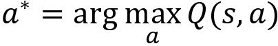 . The policy selects the best action
  with probability
  and random action with probability
- Generate an episode using policy
As we can observe, in every iteration, we generate the episode using the policy ![]() and also we try to improve the same policy
and also we try to improve the same policy ![]() in every iteration to compute the optimal policy.
in every iteration to compute the optimal policy.
Implementing on-policy MC control
Now, let's learn how to implement the MC control method with the epsilon-greedy policy to play the blackjack game; that is, we will see how can we use the MC control method to find the optimal policy in the blackjack game.
First, let's import the necessary libraries:
import gym
import pandas as pd
import random
from collections import defaultdict
Create a blackjack environment:
env = gym.make('Blackjack-v0')
Initialize the dictionary for storing the Q values:
Q = defaultdict(float)
Initialize the dictionary for storing the total return of the state-action pair:
total_return = defaultdict(float)
Initialize the dictionary for storing the count of the number of times a state-action pair is visited:
N = defaultdict(int)
Define the epsilon-greedy policy
We learned that we select actions based on the epsilon-greedy policy, so we define a function called epsilon_greedy_policy, which takes the state and Q value as an input and returns the action to be performed in the given state:
def epsilon_greedy_policy(state,Q):
Set the epsilon value to 0.5:
epsilon = 0.5
Sample a random value from the uniform distribution; if the sampled value is less than epsilon then we select a random action, else we select the best action that has the maximum Q value as shown:
    if random.uniform(0,1) < epsilon:
        return env.action_space.sample()
    else:
        return max(list(range(env.action_space.n)), key = lambda x: Q[(state,x)])
Generating an episode
Now, let's generate an episode using the epsilon-greedy policy. We define a function called generate_episode, which takes the Q value as an input and returns the episode.
First, let's set the number of time steps:
num_timesteps = 100
Now, let's define the function:
def generate_episode(Q):
Initialize a list for storing the episode:
episode = []
Initialize the state using the reset function:
state = env.reset()
Then for each time step:
for t in range(num_timesteps):
Select the action according to the epsilon-greedy policy:
action = epsilon_greedy_policy(state,Q)
Perform the selected action and store the next state information:
next_state, reward, done, info = env.step(action)
Store the state, action, and reward in the episode list:
episode.append((state, action, reward))
If the next state is the final state then break the loop, else update the next state to the current state:
        if done:
            break

        state = next_state
    return episode
Computing the optimal policy
Now, let's learn how to compute the optimal policy. First, let's set the number of iterations, that is, the number of episodes, we want to generate:
num_iterations = 500000
For each iteration:
for i in range(num_iterations):
We learned that in the on-policy control method, we will not be given any policy as an input. So, we initialize a random policy in the first iteration and improve the policy iteratively by computing the Q value. Since we extract the policy from the Q function, we don't have to explicitly define the policy. As the Q value improves, the policy also improves implicitly. That is, in the first iteration, we generate the episode by extracting the policy (epsilon-greedy) from the initialized Q function. Over a series of iterations, we will find the optimal Q function, and hence we also find the optimal policy.
So, here we pass our initialized Q function to generate an episode:
episode = generate_episode(Q)
Get all the state-action pairs in the episode:
all_state_action_pairs = [(s, a) for (s,a,r) in episode]
Store all the rewards obtained in the episode in the rewards list:
rewards = [r for (s,a,r) in episode]
For each step in the episode:
for t, (state, action,_) in enumerate(episode):
If the state-action pair is occurring for the first time in the episode:
if not (state, action) in all_state_action_pairs[0:t]:
Compute the return R of the state-action pair as the sum of rewards, R(st, at) = sum(rewards[t:]):
R = sum(rewards[t:])
Update the total return of the state-action pair as total_return(st, at) = total_return(st, at) + R(st, at):
total_return[(state,action)] = total_return[(state,action)] + R
Update the number of times the state-action pair is visited as N(st, at) = N(st, at) + 1:
N[(state, action)] += 1
Compute the Q value by just taking the average, that is,
Q[(state,action)] = total_return[(state, action)] / N[(state, action)]
Thus on every iteration, the Q value improves and so does the policy.
After all the iterations, we can have a look at the Q value of each state-action pair in the pandas data frame for more clarity. First, let's convert the Q value dictionary into a pandas data frame:
df = pd.DataFrame(Q.items(),columns=['state_action pair','value'])
Let's look at the first few rows of the data frame:
df.head(11)
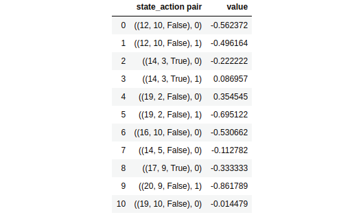
Figure 4.23: The Q values of the state-action pairs
As we can observe, we have the Q values for all the state-action pairs. Now we can extract the policy by selecting the action that has the maximum Q value in each state. For instance, say we are in the state (21,8, True). Now, should we perform action 0 (stand) or action 1 (hit)? It makes more sense to perform action 0 (stand) here, since the value of the sum of our cards is already 21, and if we perform action 1 (hit) our game will lead to a bust.
Note that due to stochasticity, you might get different results than those shown here.
Let's look at the Q values of all the actions in this state, (21,8, True):
df[124:126]
The preceding code will print the following:

Figure 4.24: The Q values of the state (21,8, True)
As we can observe, we have a maximum Q value for action 0 (stand) compared to action 1 (hit). So, we perform action 0 in the state (21,8, True). Similarly, in this way, we can extract the policy by selecting the action in each state that has the maximum Q value.
In the next section, we will learn about an off-policy control method that uses two different policies.
Off-policy Monte Carlo control
Off-policy Monte Carlo is another interesting Monte Carlo control method. In the off-policy method, we use two policies called the behavior policy and the target policy. As the name suggests, we behave (generate episodes) using the behavior policy and we try to improve the other policy called the target policy.
In the on-policy method, we generate an episode using the policy ![]() and we improve the same policy
and we improve the same policy ![]() iteratively to find the optimal policy. But in the off-policy method, we generate an episode using a policy called the behavior policy b and we try to iteratively improve a different policy called the target policy
iteratively to find the optimal policy. But in the off-policy method, we generate an episode using a policy called the behavior policy b and we try to iteratively improve a different policy called the target policy ![]() .
.
That is, in the on-policy method, we learned that the agent generates an episode using the policy ![]() . Then for each step in the episode, we compute the return of the state-action pair and compute the Q function Q(st, at) as an average return, then from this Q function, we extract a new policy
. Then for each step in the episode, we compute the return of the state-action pair and compute the Q function Q(st, at) as an average return, then from this Q function, we extract a new policy ![]() . We repeat this step iteratively to find the optimal policy
. We repeat this step iteratively to find the optimal policy ![]() .
.
But in the off-policy method, the agent generates an episode using a policy called the behavior policy b. Then for each step in the episode, we compute the return of the state-action pair and compute the Q function Q(st, at) as an average return, then from this Q function, we extract a new policy called the target policy ![]() . We repeat this step iteratively to find the optimal target policy
. We repeat this step iteratively to find the optimal target policy ![]() .
.
The behavior policy will usually be set to the epsilon-greedy policy and thus the agent explores the environment with the epsilon-greedy policy and generates an episode. Unlike the behavior policy, the target policy is set to be the greedy policy and so the target policy will always select the best action in each state.
Let's now understand how the off-policy Monte Carlo method works exactly. First, we will initialize the Q function with random values. Then we generate an episode using the behavior policy, which is the epsilon-greedy policy. That is, from the Q function we select the best action (the action that has the max Q value) with probability 1-epsilon and we select the random action with probability epsilon. Then for each step in the episode, we compute the return of the state-action pair and compute the Q function Q(st, at) as an average return. Instead of using the arithmetic mean to compute the Q function, we can use the incremental mean. We can compute the Q function using the incremental mean as shown as follows:
After computing the Q function, we extract the target policy ![]() by selecting an action in each state that has the maximum Q value as shown as follows:
by selecting an action in each state that has the maximum Q value as shown as follows:

The algorithm is given as follows:
- Initialize the Q function Q(s, a) with random values, set the behavior policy b to be epsilon-greedy, and also set the target policy to be greedy policy.
- For M number of episodes:
- Generate an episode using the behavior policy b
- Initialize return R to 0
- For each step t in the episode, t = T-1, T-2,…, 0:
- Compute the return as R = R+rt+1
- Compute the Q value as
- Compute the target policy
- Return the target policy

As we can observe from the preceding algorithm, first we set the Q values of all the state-action pairs to random values and then we generate an episode using the behavior policy. Then on each step of the episode, we compute the updated Q function (Q values) using the incremental mean and then we extract the target policy from the updated Q function. As we can notice, on every iteration, the Q function is constantly improving and since we are extracting the target policy from the Q function, our target policy will also be improving on every iteration.
Also, note that since it is an off-policy method, the episode is generated using the behavior policy and we try to improve the target policy.
But wait! There is a small issue here. Since we are finding the target policy ![]() from the Q function, which is computed based on the episodes generated by a different policy called the behavior policy, our target policy will be inaccurate. This is because the distribution of the behavior policy and the target policy will be different. So, to correct this, we introduce a new technique called importance sampling. This is a technique for estimating the values of one distribution when given samples from another.
from the Q function, which is computed based on the episodes generated by a different policy called the behavior policy, our target policy will be inaccurate. This is because the distribution of the behavior policy and the target policy will be different. So, to correct this, we introduce a new technique called importance sampling. This is a technique for estimating the values of one distribution when given samples from another.
Let us say we want to compute the expectation of a function f(x) where the value of x is sampled from the distribution p(x) that is,  ; then we can write:

With the importance sampling method, we estimate the expectation using a different distribution q(x); that is, instead of sampling x from p(x) we use a different distribution q(x) as shown as follows:
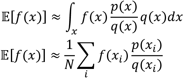
The ratio 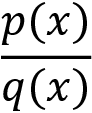 is called the importance sampling ratio or importance correction.
Okay, how does importance sampling help us? We learned that with importance sampling, we can estimate the value of one distribution by sampling from another using the importance sampling ratio. In off-policy control, we can estimate the target policy with the samples (episodes) from the behavior policy using the importance sampling ratio.
Importance sampling has two types:
- Ordinary importance sampling
- Weighted importance sampling
In ordinary importance sampling, the importance sampling ratio will be the ratio of the target policy to the behavior policy 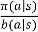 and in weighted importance sampling, the importance sampling ratio will be the weighted ratio of the target policy to the behavior policy
  .
.
Let's now understand how we use weighted importance sampling in the off-policy Monte Carlo method. Let W be the weight and C(st, at) denote the cumulative sum of weights across all the episodes. We learned that we compute the Q function (Q values) using the incremental mean as:
Now, we slightly modify our Q function computation with the weighted importance sampling as shown as follows:
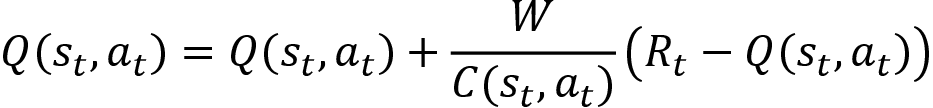
The algorithm of the off-policy Monte Carlo method is shown next. First, we generate an episode using the behavior policy and then we initialize return R to 0 and the weight W to 1. Then on every step of the episode, we compute the return and update the cumulative weight as C(st, at) = C(st, at) + W. After updating the cumulative weights, we update the Q value as .
From the Q value, we extract the target policy as . When the action at given by the behavior policy and the target policy is not the same then we break the loop and generate the next episode; else we update the weight as  .
.
The complete algorithm of the off-policy Monte Carlo method is explained in the following steps:
- Initialize the Q function Q(s, a) with random values, set the behavior policy b to be epsilon-greedy, and target policy to be greedy policy and initialize the cumulative weights as C(s, a) = 0
- For M number of episodes:
- Return the target policy

 then break
Is the MC method applicable to all tasks?
We learned that Monte Carlo is a model-free method, and so it doesn't require the model dynamics of the environment to compute the value and Q function in order to find the optimal policy. The Monte Carlo method computes the value function and Q function by just taking the average return of the state and the average return of the state-action pair, respectively.
But one issue with the Monte Carlo method is that it is applicable only to episodic tasks. We learned that in the Monte Carlo method, we compute the value of the state by taking the average return of the state and the return is the sum of rewards of the episode. But when there is no episode, that is, if our task is a continuous task (non-episodic task), then we cannot apply the Monte Carlo method.
Okay, how do we compute the value of the state where we have a continuous task and also where we don't know the model dynamics of the environment? Here is where we use another interesting model-free method called temporal difference learning. In the next chapter, we will learn exactly how temporal difference learning works.
Summary
We started the chapter by understanding what the Monte Carlo method is. We learned that in the Monte Carlo method, we approximate the expectation of a random variable by sampling, and when the sample size is greater, the approximation will be better. Then we learned about the prediction and control tasks. In the prediction task, we evaluate the given policy by predicting the value function or Q function, which helps us to understand the expected return an agent would get if it uses the given policy. In the control task, our goal is to find the optimal policy, and we will not be given any policy as input, so we start by initializing a random policy and we try to find the optimal policy iteratively.
Moving forward, we learned how to use the Monte Carlo method to perform the prediction task. We learned that the value of a state and the value of a state-action pair can be computed by just taking the average return of the state and an average return of state-action pair across several episodes, respectively.
We also learned about the first-visit MC and every-visit MC methods. In first-visit MC, we compute the return only for the first time the state is visited in the episode, and in every-visit MC, we compute the return every time the state is visited in the episode.
Following this, we explored how to perform a control task using the Monte Carlo method. We learned about two different types of control methods—on-policy and off-policy control.
In the on-policy method, we generate episodes using one policy and also improve the same policy iteratively to find the optimal policy. We first learned about the Monte Carlo control exploring starts method where we set all the state-action pairs to a non-zero probability to ensure exploration. Later, we learned about Monte Carlo control with an epsilon-greedy policy where we select a random action (exploration) with probability epsilon, and with probability 1-epsilon we select the best action (exploitation).
At the end of the chapter, we discussed the off-policy Monte Carlo control method where we use two different policies called the behavior policy, for generating the episode, and the target policy, for finding the optimal policy.
Questions
Let's assess our knowledge of the Monte Carlo methods by answering the following questions:
- What is the Monte Carlo method?
- Why is the Monte Carlo method preferred over dynamic programming?
- How do prediction tasks differ from control tasks?
- How does the MC prediction method predict the value function?
- What is the difference between first-visit MC and every-visit MC?
- Why do we use incremental mean updates?
- How does on-policy control differ from off-policy control?
- What is the epsilon-greedy policy?