
9
Skin–Stiffened Structure
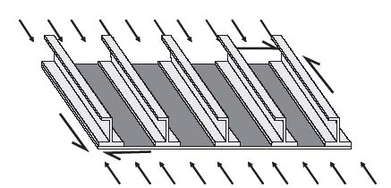
The individual constituents, skin and stiffeners, have been examined in previous chapters. Based on that discussion, the behaviour and the design of a stiffened panel such as the one shown in Figure 9.1 can be summarized as follows: The skin takes pressure loads via in-plane stretching (membrane action) and shear loads. It also takes compression loads up to buckling. Beyond buckling, extra care must be exercised to account for the skin deformations and additional failure modes, not examined so far, such as the skin–stiffener separation, which is discussed in this chapter. The stiffeners take bending and compression loads. It is readily apparent that the robustness and efficiency of a design will strongly depend on how one can ‘sequence’ the various failure modes so benign failures occur first and load can be shared by the rest of the structure, and how one can eliminate certain failure modes without unduly increasing the weight of the entire panel.
Figure 9.1 Stiffened panel under combined loads
In this chapter, some aspects that manifest themselves at the component level, with both skin and stiffeners present, are examined. This includes modelling aspects such as smearing of stiffness properties and additional failure modes such as the skin–stiffener separation.
9.1 Smearing of Stiffness Properties (Equivalent Stiffness)
If the number of stiffeners is sufficiently large and/or their spacing is sufficiently narrow, accurate results for the overall panel performance can be obtained by smearing the skin and stiffener properties in combined, equivalent stiffness, expressions. This can be done for both in-plane (membrane) and out-of-plane (bending) properties.
9.1.1 Equivalent Membrane Stiffnesses
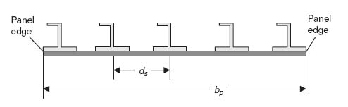
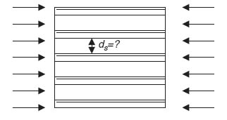
A composite stiffened panel is shown in Figure 9.2. The stiffener spacing is ds and the width of the panel is bp.
Figure 9.2 Section cut of a composite stiffened panel
As can be seen from Equation (8.13), the equivalent in-plane stiffness of the skin–stiffener combination is the sum of the individual stiffnesses of skin and stiffeners. This means that the A matrix for the entire panel, which is the membrane stiffness per unit width, is given by the sum of the corresponding terms for skin and stiffeners considered separately:
with the subscript ij denoting the ij element of the A matrix. Also, again from Equation (8.13),
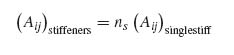
where ns is the number of stiffeners.
Determining the number of stiffeners involves some approximation caused by the presence or lack of stiffeners at the panel edges. If there are stiffeners right at the panel edges as in Figure 9.2, the number of stiffeners is given by
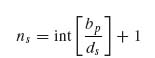
where int […] denotes the integer that is obtained when the quantity in brackets is rounded down to the nearest integer.
If the stiffener spacing is sufficiently small, the second term in the right-hand side of Equation (9.3) can be neglected and the number of stiffeners approximated by

If there are no stiffeners at the panel edges, that is, the skin overhangs on either side of the panel, bp in Equation (9.3) must be reduced by the total amount of overhang. Again, for sufficiently large bp and/or small ds Equation (9.4) can be used. Note that Equation (9.4) is typically a rational number as the division bp/ds is an integer only for judiciously chosen values of bp and ds. But, for the purpose of stiffness estimation, using the rational number obtained from Equation (9.4) without round-off is a reasonable approximation.
Now the Aij term for a single stiffener can be estimated by averaging the corresponding membrane stiffness of the stiffener over the skin width bp. For the case of A11 this gives
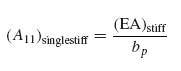
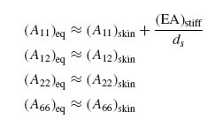
Placing Equations (9.2), (9.4) and (9.5) into Equation (9.1) and recognizing that a one-dimensional stiffener has negligible contribution to stiffnesses other than the one parallel to its own axis gives the A matrix terms:
9.1.2 Equivalent Bending Stiffnesses
The derivation of the bending stiffnesses proceeds in a similar fashion. Based on Equation (8.20) the bending stiffnesses per unit width can be written as
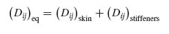
with
(9.8) 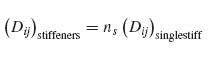
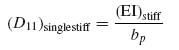
The bending stiffness D11 for a single stiffener can be determined by smearing its contribution over the entire width bp:
While there are no contributions to the D12 and D22 terms because the bending stiffness contribution from the stiffeners is negligible in these directions, the contribution to D66 requires a detailed derivation.
Consider the situation shown in Figure 9.3 where a laminate deforms under an applied torque.
Figure 9.3 Laminate under applied torque
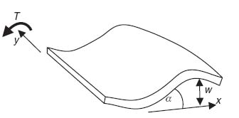
The angle α is given by
From torsion theory [1], the rate of change of angle α as a function of y is given by

where T is the applied torque, G the shear modulus and J the torsional rigidity. Combining Equations (9.10) and (9.11) gives
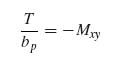
Now from classical laminated-plate theory (see Equation 3.49 and assuming no coupling is present) the torque per unit width Mxy is given by
Since now
Equations (9.12), (9.13) and (9.14) can be combined and applied to a single stiffener to give
(9.15) 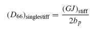
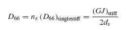
This equation is analogous to Equation (9.9), but there is a factor of 2 in the denominator. Summing up the contributions of all stiffeners and using Equation (9.4), the contribution of all stiffeners to D66 for the combined skin–stiffener configuration is
Finally, combining Equations (9.7) to (9.9) and (9.16) gives the final approximate expressions for the bending stiffnesses of a stiffened panel:
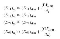
which are analogous to Equations (9.6) in the previous section.
If the stiffeners have an open cross-section (such as L, C, Z, T, I, J) the torsional rigidity J in the last of Equations (9.17) is negligibly small and the stiffener contribution (second term in that equation) can be neglected altogether. If the stiffeners have a closed cross-section (such as a hat stiffener) the second term in the last of Equations (9.17) is significant and cannot be neglected.
In addition to the approximation introduced by Equation (9.4) when the number of stiffeners is small, there is an approximation in Equations (9.17) introduced by the fact that stretching–bending coupling terms (B matrix contribution) were neglected. The skin–stiffener cross-section in Figure 9.2 is asymmetric and there is a contribution to the bending stiffnesses coming from the axial stiffnesses of the stiffeners and skin. These are analogous to the B matrix terms of an asymmetric laminate and they become more significant as the stiffeners become bigger (e.g. greater web heights). Only in a situation where the stiffeners are mirrored to the other side of the skin, giving a symmetric configuration with respect to the skin mid-plane, will these coupling terms be exactly zero and no additional correction terms needed in Equation (9.17).
9.2 Failure Modes of a Stiffened Panel
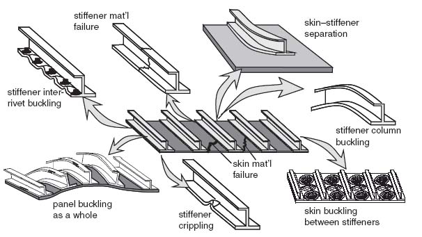
Failure modes that are specific to the individual constituents, skin and stiffeners, were examined in previous chapters. Here, a summary of all failure modes, including those pertaining to the interaction between the skin and stiffeners, is given. The most important failure modes are presented in Figure 9.4. Of these, the material strength failure modes (either for the stiffener or for the skin) are typically covered by a first-ply failure analysis (see Chapter 4) supported and modified by test results. They were also briefly invoked in the discussion on crippling (Section 8.5) and skin post-buckling (see Sections 7.1 and 7.2). Flange crippling was examined in Section 8.5. Inter-rivet buckling was discussed in Section 8.7. Panel buckling failure modes were discussed in Chapter 6 for plates and Section 8.3 for beams. Whichever buckling mode occurs first, overall buckling of the panel or buckling of the skin between stiffeners is a function of the relative stiffnesses and geometry of skin and stiffeners, and conditions ensuring precedence of one buckling mode over another are discussed in this chapter. Finally, the skin–stiffener separation mode was briefly mentioned in association with post-buckling (at the start of Chapter 7) and will be examined in detail in this chapter.
Figure 9.4 Failure modes of a stiffened panel
As might be expected, unless explicitly designed for this, failure modes do not occur simultaneously. In certain situations, designing so that some (or all) failure modes occur at the same time gives the most efficient design in the sense that no component is over-designed. This is not always true. It assumes that different components are used to take different types of loading and fail in different failure modes that are independent of one another. In general, formal optimization shows that the lightest designs are not always the ones where the critical failure modes occur simultaneously.
In view of this, knowing when one failure mode may switch to another is critical. In addition, sequencing failure modes so they occur in a predetermined sequence is also very useful for the creation of robust designs. For example, relatively benign failure modes such as crippling (as opposed to column buckling) and local buckling between stiffeners (as opposed to overall buckling) contribute to creating a damage-tolerant design, in the sense that catastrophic failure is delayed and some load sharing with components that have not yet failed occurs. One such case of finding when one failure mode changes to another was examined in Section 8.7 where the condition for switching from crippling to inter-rivet buckling was determined.
9.2.1 Local Buckling (between Stiffeners) versus Overall Panel Buckling (the Panel Breaker Condition)
As mentioned in the previous section, confining the buckling mode between stiffeners is preferable. In general it leads to lighter designs and keeps the overall panel from buckling, which, typically, leads to catastrophic failure. From a qualitative point of view, as the bending stiffness of the stiffeners increases, it becomes harder for them to bend. Then under compressive loading, for example, if the stiffeners are sufficiently stiff, the skin between the stiffeners will buckle first. The stiffeners remain straight and act as ‘panel breakers’. For a given stiffener stiffness, this behaviour can be assured if the stiffener spacing is sufficiently wide. Then, even for relatively soft stiffeners, the skin between them will buckle first. This means that the panel breaker condition will involve both the stiffness and spacing of the stiffeners compared with the skin stiffness and its overall dimensions.
There are two main scenarios to quantify this sequence of events. In the first, a non-buckling design is all that is required (no post-buckling capability). In such a case, the stiffeners must have properties such that the buckling load of the panel as a whole equals the buckling load of the skin between stiffeners. The two failure modes, local and global buckling, occur simultaneously. In the second scenario, the skin is allowed to buckle. This means that the stiffeners must stay intact and not bend, until the skin reaches the desired post-buckling load and fails.
9.2.1.1 Global Buckling = Local Buckling (Compression Loading)
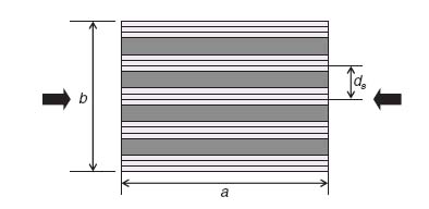
It is important to recognize that the total applied force FTOT is distributed between the skin and stiffeners according to their respective in-plane EA stiffnesses. This was expressed by Equation (8.12). With reference to Figure 9.5, the membrane stiffness EA of the skin is approximated by bA11. Note that a more accurate expression would be b(A11 − A122/A22), as is indicated by Equations (8.5) and (8.6), but the second term is neglected here, assuming the skin has at least 40% 0° plies aligned with the load so that A12 ![]() A11. If this requirement is not satisfied, the equations that follow can be modified accordingly.
A11. If this requirement is not satisfied, the equations that follow can be modified accordingly.
Figure 9.5 Stiffened skin under compression
Using Equation (8.12), the force acting on the skin alone can be determined as
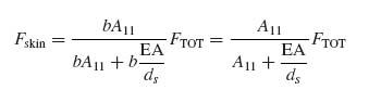
It should be emphasized that FTOT here refers to the total force on both skin and stiffeners. This is different than Equations (8.8), (8.9), (8.10), (8.11) and (8.12) where FTOT referred to the total force on the stiffener alone.
Then, the force per unit length acting on the skin alone is
(9.19) 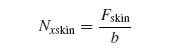
If the skin between stiffeners is assumed to be simply supported, its buckling load can be obtained from Equation (6.7):

where k is the number of half-waves into which the skin buckles, Dij are skin bending stiffnesses and ![]() is the aspect ratio a/ds.
is the aspect ratio a/ds.
Combining Equations (9.18) to (9.20) and solving for the total force FTOT gives
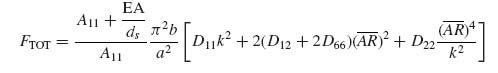
where A11 is the skin membrane stiffness and EA is the stiffener membrane stiffness.
Assuming now that the panel as a whole is simply supported all around its boundary, its buckling load will also be given by Equation (6.7):
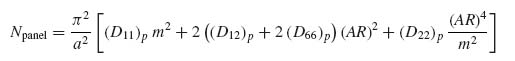
where m is the number of half-waves into which the entire panel would buckle (note that m for the overall panel and k for the skin between the stiffeners can be different) and the subscript p denotes the entire panel. The aspect ratio AR of the panel is a/b. The bending stiffnesses (Dij)p for the panel are given by Equation (9.17).
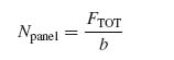
The force per unit length Npanel is given by
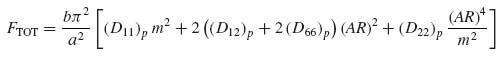
Combining Equations (9.22) and (9.23) and solving for FTOT gives
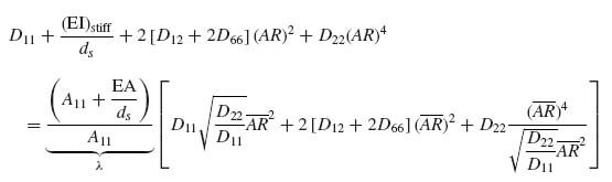
Equations (9.21) and (9.24) imply that the total load at which the skin between stiffeners buckles and the panel as a whole buckles is the same. Therefore, equating the right-hand sides of Equations (9.21) and (9.24) gives
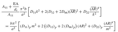
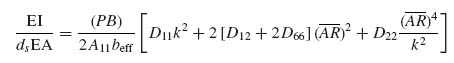
Equation (9.25) can be simplified by cancelling out common factors and using Equation (9.17) to express the panel bending stiffnesses EI. Here, it will be assumed that the stiffener has an open cross-section so its GJ is very small and does not contribute to the panel D66 value. Then, Equation (9.25) reads
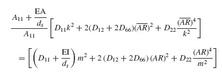
Note that, in Equation (9.26), EA and EI both refer to stiffener quantities.
Further simplification is possible if the values of k and m are approximated. As mentioned in Section 6.2, k and m are the integer values of half-waves that minimize the corresponding buckling loads (skin between stiffeners or entire panel). If k and m were continuous variables (instead of only taking integer values) differentiating the corresponding buckling expressions and setting the result equal to zero would give the values to use (see the derivation of Equation 8.45). Since they are integers, the rational expression resulting from differentiation would have to be rounded up or down to the nearest adjacent integer that minimizes the buckling load.
Differentiating the right-hand side of Equation (9.20) with respect to k and setting the result equal to zero gives
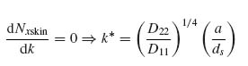
where k* denotes the continuous variable (k = k* when the right-hand side of Equation 9.27 is an integer).
Using Equation (9.27), the value of k is given by either
![]()
or
![]()
whichever of the two minimizes the right-hand side of Equation (9.20). The symbol int[x] denotes the integer obtained if x is rounded down to the next integer.
Similarly for m,
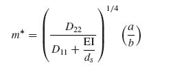
By necessity, if either of k* or m* is less than 1, the corresponding value of k or m will be set equal to 1.
Now for typical applications of panels under compression, the quantity D11 + EI/ds is greater than D22 because of the contribution of the stiffeners EI/ds and the tendency to align fibres with the load direction which would give D11 ≥ D22. So unless a/b ![]() 1 the quantity in the right-hand side of Equation (9.28) is less than 1 and m will be equal to 1.
1 the quantity in the right-hand side of Equation (9.28) is less than 1 and m will be equal to 1.
To proceed, set k = k* as obtained from Equation (9.27). Then, substituting for k and m in Equation (9.26)
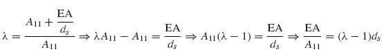
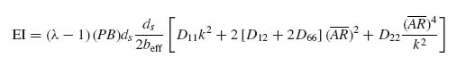
Denoting by λ the term multiplying the quantity in brackets on the right-hand side, solving for the stiffener EI, and dropping the subscript ‘stiff’, for convenience, gives the final expression:
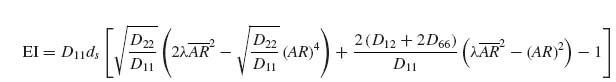
Equation (9.30) gives the minimum bending stiffness EI that the stiffeners must have in order for buckling of the skin between stiffeners to occur at the same time as overall buckling of the stiffened panel. If EI is greater than the right-hand side of Equation (9.30), the skin between stiffeners buckles first.
9.2.1.2 Stiffener Buckling = PB × Buckling of Skin between Stiffeners (Compression Loading)
This scenario covers the case where skin is allowed to post-buckle. It is assumed that the skin is loaded over the beff portion, which was determined in Section 7.1. The stiffener must stay straight all the way up to the load that fails the skin. That load is given by the buckling load of the skin between stiffeners multiplied by the post-buckling ratio PB.
Figure 9.6 Effective skin in the vicinity of a stiffener in a post-buckled stiffened panel
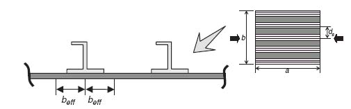
In general, when the skin has buckled the compressive load on it is not constant (see Figure 7.8 for example) and the skin strains are not constant across its width. If the skin is replaced by the beff portion shown in Figure 9.6, then the skin load is constant over beff and the strain, given by inverting Equation (8.4), is also constant. Thus, strain compatibility can be applied.
Considering a 2beff portion of skin and its corresponding stiffener as shown in Figure 9.6 and using Equation (8.12), the individual forces on skin and stiffener can be found to be
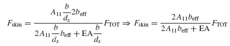
where EA is the membrane stiffness of each stiffener (= membrane modulus × cross-sectional area)
For a single stiffener, dividing the right-hand side of Equation (9.32) by the number of stiffeners given by Equation (9.4) gives
Now, the column buckling load of a stiffener is, for simply supported ends, given by Equation (8.21), repeated here for convenience:
Equating the right-hand sides of Equations (9.33) and (9.34) relates the load in each stiffener to the buckling load of that stiffener and can be solved for the total force on the panel FTOT:
Now it is postulated that final failure occurs when the required post-buckling ratio PB is reached. At that point, the force in the skin Fskin must equal the buckling load of the skin between the stiffeners multiplied by PB:
The skin buckling load Fskinbuckling is given by Equation (9.20) multiplied by the panel width b to convert the force per unit width Nxskin into force:
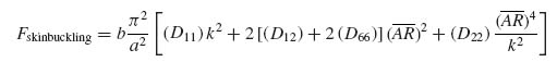
with all terms as defined before.
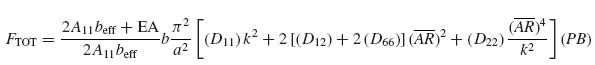
Combining Equation (9.31) with Equations (9.36) and (9.37) relates the total force to the skin buckling load:
Equations (9.35) and (9.38) can now be combined to yield the condition for column buckling of the stiffeners occurring when the final PB is reached:
which relates stiffener properties on the left-hand side with skin properties on the right-hand side.
Equation (9.39) can be further manipulated using the definition of the parameter λ that was introduced when Equation (9.29) was derived. Using that definition, it can be shown that
Introducing this result in Equation (9.39) and solving for the stiffener bending stiffness EI results in the expression
Also note that using the expression for beff, Equation (7.15), derived earlier (assuming the boundary conditions for the skin between stiffeners reasonably approximate those used in Section 7.1) the following can be shown:
(9.42) 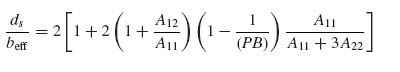
which can be substituted in Equation (9.41).
Equation (9.41) determines the minimum bending stiffness of the stiffeners so that they do not buckle until the final failure load in the post-buckling regime is reached. This would guarantee that the stiffeners will stay straight and thus act as panel breakers, all the way to the failure load of the panel. It should be noted that EI in Equation (9.41) is related to the stiffener EA through the parameter λ so the two are not entirely independent and some iterations may be needed between stiffener geometry and layup to arrive at the required bending stiffness.
9.2.1.3 Example
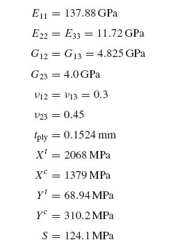
As an application of the two conditions (9.30) and (9.41) consider a skin panel with dimensions a = 508 mm and b = 762 mm loaded in compression parallel to dimension a as shown in Figure 9.7. The skin layup is [(±45)/(0/90)/(±45)] with stiffness properties given in Figure 9.7. The stiffener spacing, geometry and layup are unknown. The minimum EI for the stiffeners must be determined subject to conditions (9.30) and (9.41).
Figure 9.7 Example of stiffened panel under compression
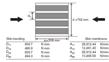
The procedure is as follows: First a value of the parameter λ is selected. Then, for that value, the stiffener spacing ds is varied between 75 and 300 mm. For each value of ds the aspect ratio (![]() ) is calculated and the corresponding buckling load of the skin between the stiffeners is determined using Equation (9.20). Finally, the minimum EI required is determined using Equations (9.30) and (9.41). When using Equation (9.41) a PB ratio of 5 is assumed. The results are shown in Figure 9.8 for two different λ values.
) is calculated and the corresponding buckling load of the skin between the stiffeners is determined using Equation (9.20). Finally, the minimum EI required is determined using Equations (9.30) and (9.41). When using Equation (9.41) a PB ratio of 5 is assumed. The results are shown in Figure 9.8 for two different λ values.
Figure 9.8 Normalized minimum bending stiffness required for stiffeners of a stiffened panel under compression (PB = 5)
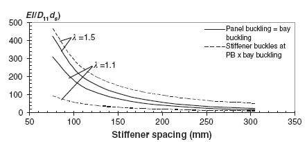
It can be seen from Figure 9.8 that the minimum bending stiffness for the stiffener decreases as the stiffener spacing increases. This is due to the fact that, as the stiffener spacing increases, the buckling load of the skin between the stiffeners decreases. This implies that the total load at which the skin buckles is lower and the corresponding load applied to the stiffeners is lower. So the stiffener requirement must be satisfied for a lower load and thus lower bending stiffness is needed.
It is also evident from Figure 9.8 that as λ decreases, the required bending stiffness for the stiffener decreases. This is because, for a given skin (and thus A11 value), the only way to decrease λ is by decreasing the stiffener EA (see Equation 9.40). But if the stiffener EA decreases, less load is absorbed by the stiffeners (see Equation 9.32) and more by the skin. Again, since the load carried by each stiffener is lower, the required bending stiffness will also be lower.
The last observation related to the trends of Figure 9.8 is that a value of λ is reached beyond which the condition that the stiffeners buckle at PB × bay buckling dominates. This is demonstrated by the fact that the continuous curve is above the dashed curve for λ = 1.1, but below the dashed curve for λ = 1.5. This means that, for a given stiffener spacing, there is a λ value between 1.1 and 1.5 at which the design driver switches from Equation (9.30) to Equation (9.41). This means that one should check both conditions, (9.30) and (9.41), and use the one that gives the more conservative results. If no post-buckling is allowed in the design, only condition (9.30) should be used.
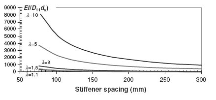
Selecting the more critical of the two conditions, for each value of λ, results in the curves of Figure 9.9. The lowest three curves (λ = 1.1, 1.5, 3.0) correspond to Equation (9.30) dominating the design and the highest two curves (λ = 5.0, 10.) correspond to Equation (9.40) dominating the design.
Figure 9.9 Normalized minimum bending stiffness of stiffeners for various λ values (PB = 5)
9.2.2 Skin–Stiffener Separation
As load is transferred between the skin and stiffeners, out-of-plane loads develop at their interface or at the flange edges. These loads develop even when the applied loads are in the plane of the skin and they can lead to separation of the stiffeners from the skin. There are two main mechanisms for the development of these out-of-plane stresses. The first is associated with the presence of any stress-free edges such as the flange edges [2–7]. Load present in one component such as the flange has to transfer to the other as the free edge is approached. The local stiffness mismatch caused by the presence of the free edge (and the differences in stacking sequence between flange and skin) creates out-of-plane stresses which are the main culprit for separation of the flange from the skin. This is shown in Figure 9.10.
Figure 9.10 Development of out-of-plane stresses at the interface between the flange and skin prior to buckling
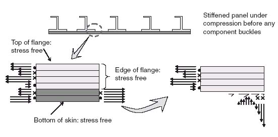
Away from the flange edge, closer to the location where the stiffener web meets the flange, a two-dimensional state of stress develops that can be determined with the use of classical laminated-plate theory once the local loads are known. A section including the flange edge and the skin below can be cut off and placed in equilibrium (bottom left part of Figure 9.10). If then the flange alone is sectioned off (bottom right of Figure 9.10), it is not in equilibrium unless out-of-plane shear and normal stresses develop at the interface between the flange and the skin. This is the only location where this can happen since the top of the flange and the right edge of the flange are, by definition, stress free. Zooming to the sectioned detail at the bottom right of Figure 9.10 gives the situation shown in Figure 9.11.
Figure 9.11 Free-body diagram of the flange
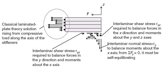
For the purposes of discussion, the skin and stiffener in Figures 9.10 and 9.11 are assumed to be under compression. A local coordinate system is established in Figure 9.11 to facilitate the discussion. As shown in Figure 9.11, to maintain force equilibrium in the y direction, an interlaminar shear stress τyz must develop at the flange–skin interface (bottom of the flange in Figure 9.11). Also, the presence of in-plane shear stresses at the left end of the flange, as predicted by the classical laminated-plate theory, leads to a net force in the x direction. In order to balance that force, an interlaminar shear stress τxz must also develop at the flange–skin interface. Finally, to balance the moments (about the bottom right corner of the flange, say), an out-of-plane normal stress σz must develop at the flange–skin interface. However, since there is no net force in the z direction in Figure 9.11, the σz stress must be self-equilibrating. Thus, it will be tensile over a portion of the region over which it acts and compressive over the remaining portion. This is why σz is shown as both tensile and compressive in Figure 9.11.
The second mechanism that gives rise to these separation stresses is associated with the skin deformation after buckling in a post-buckling situation. This is shown in Figure 9.12 based on an example from [8].
Figure 9.12 Post-buckled shape of blade-stiffened panel under compression
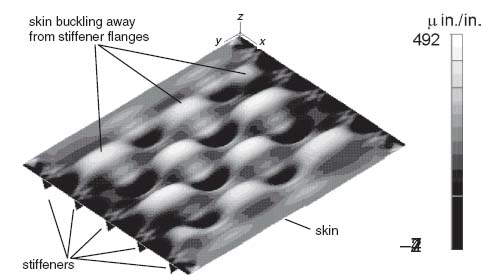
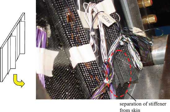
The stiffened panel of Figure 9.12 is shown with the stiffeners at the bottom so the skin deformations are more easily seen without stiffeners blocking the view. As shown in Figure 9.12 a portion of the buckling pattern has the skin moving away from the stiffeners. This would give rise to ‘peeling’ stresses at the skin–stiffener interface and could lead to skin–stiffener separation. The resulting failure for this situation is shown in Figure 9.13. The separated stiffener is highlighted with an ellipse. It is important to bear in mind that, for this mechanism to occur, buckling of the skin (under compression, shear or combined loads) is a prerequisite [9].
Figure 9.13 Skin–stiffener separation failure mode
Many different solutions to the problem of determining the stresses between the skin and stiffener given a loading situation have been proposed [2–12]. The highest accuracy is obtained with detailed finite element methods [8–12] at a relatively high computational cost. The required mesh refinement in the region (or interface) of interest makes it difficult to use this approach in a design environment where many configurations must be rapidly compared with each other for the best candidates to emerge. Simpler methods [2–6] can be used for screening candidate designs and performing a first evaluation. Once the best candidates are selected, more detailed analysis methods using finite elements can be used for more accurate predictions.
In general, solutions that calculate the stresses at the skin–stiffener interface assume a perfect bond between the stiffener flange and the skin and require the use of some out-of-plane failure criterion [13, 14] to determine when delamination starts. This can be quite conservative as a delamination starting at the skin–stiffener interface rarely grows in an unstable fashion to cause final failure. To model the presence of a delamination and to determine when it will grow, methods based on energy release rate calculations [10–12] are very useful. In what follows, only the problem of determining the out-of-plane stresses in a pristine structure will be presented.
The approach is adapted from [3, 4] and can be applied to any situation for which the loads away from the flange edge are known, irrespective of whether the structure is post-buckled or not. The situation is shown in Figure 9.14. The flange end is isolated from the rest of the stiffener and a portion of the skin below it is shown.
Figure 9.14 Geometry and coordinate systems for the skin–stiffener separation problem
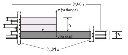
Two coordinate systems are used in Figure 9.14, one for the flange and one for the skin. They have a common origin at the end of the flange where it interfaces with the skin. The z axis (out-of-plane) for the flange is going up while it is going down for the skin. The y axis is moving away from the flange edge towards the stiffener web and the x axis is aligned with the axis of the stiffener. The stresses away from the origin of the coordinate systems, at the far left and right end in Figure 9.14, are assumed known. They would be the result of classical laminated-plate theory and/or other two-dimensional solutions. For the solution discussed here, these far-field stresses are assumed to be only in-plane stresses. This means that the three-dimensional stresses that arise in the vicinity of the flange termination die out in the far field so the known solution at the left and right ends of Figure 9.14 can be recovered. Note that out-of-plane stresses at the far field can, if present, be added following the same procedure as the one outlined below.
It is assumed that the structure shown in Figure 9.14 is long in the x direction (perpendicular to the plane of the figure) so no quantity depends on the x coordinate, that is,
![]()
With this assumption, the equilibrium equations (5.2) become
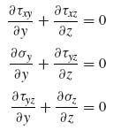
This means that the first equilibrium equation, (9.43a), uncouples from the other two. This, in turn, suggests that if one of the stresses τxy or τxz were somehow known, Equation (9.43a) could be used to determine the other. Similarly, if one of the stresses σy, τyz or σz were known, the other two could be determined from Equations (9.43b) and (9.43c).
Pursuing this line of thought, a fairly general assumption is made for τxy and σy in the form
where f(y), g(y), F(z) and G(z) are unknown functions of the respective coordinates and (σy(z))ff and (τxy(z))ff are the known far-field stresses away from the flange edge (i.e. at large positive or negative y values).
The solution remains quite general if F(z) and G(z) are assumed to be Fourier sine and cosine series. Concentrating on the flange, Equations (9.44) and (9.45) can be written as
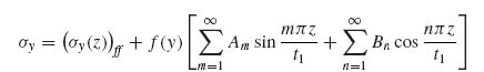
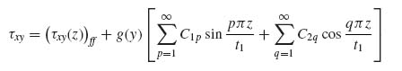
Here a simplification is introduced by truncating the infinite series in Equations (9.44a) and (9.45a) after the first term. This will give good solutions in terms of trends and will simplify the algebra considerably. Additional terms may be included for more accurate solutions. Then the two stresses in the flange have the form
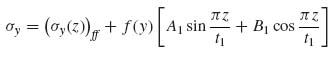
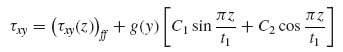
where, for simplicity, we set C1 = C11 and C2 = C21. The coefficients A1, B1, C1 and C2 and the functions f(y) and g(y) are unknown at this point.
Now use Equation (9.44b) to substitute in Equation (9.43b) to obtain
where f′ = df/dy.
Integrating Equation (9.46) with respect to z gives
(9.47) 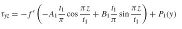
where P1(y) is an unknown function of y.
Now the top of the flange is stress free, which means that τyz(z = t1) = 0 or,
(9.48) 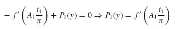
and P1(y) is determined. This would give the following expression for τyz:
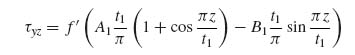
In a similar fashion, Equation (9.49) can be used to substitute for τyz in Equation (9.43c) to obtain
(9.50) 
which can be integrated with respect to z to give
where f′′ = d2f/dy2 and P2(y) is an unknown function.
Again, the requirement that the top of the flange be stress free leads to σz(z = t1) = 0 or
(9.52) 
With P2(y) known, the final expression for σz can be obtained:
(9.53) 
In a completely analogous fashion, placing Equation (9.45b) into Equation (9.43a) and solving for τxz gives
Equations (9.44b), (9.45b), (9.49), (9.51) and (9.54) determine the stresses σy, τxy, τyz, σz and τxz to within some unknown constants and the two unknown functions f and g and their derivatives. At this point the stress σx is unknown. It does not appear in the equilibrium equations (9.43a–c) and other means must be invoked for its determination.
By inverting the stress–strain equations (5.4), the following relations are obtained:
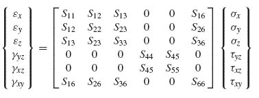
where Sij (i, j = 1–6) are compliances for the flange as a whole. They can be computed as thickness-averaged sums of the corresponding compliances for the individual plies, and the compliances of the individual plies are obtained using standard tensor transformation equations (Equations 3.8–3.10).
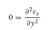
In addition, the strain compatibility relations (5.10) and (5.12) can be rewritten as
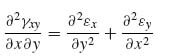
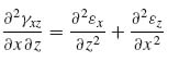
As was mentioned earlier, there is no dependence on the x coordinate so all derivatives with respect to x are zero and Equations (9.56) and (9.57) simplify to

The first of Equations (9.55) can be combined with Equations (9.58) and (9.59) to give
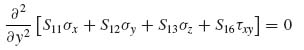
The quantity in brackets is the same for both Equations (9.60) and (9.61). The only way these two equations can be compatible with each other is if the quantity in brackets has the following form:
with G1(z) and G2(z) unknown functions of z.
Using Equation (9.62) to substitute in Equation (9.61) gives
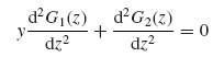
from which
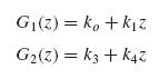
with ko, k1, k3 and k4 unknown constants.
Using this result and Equation (9.62) to solve for σx gives
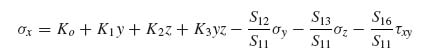
with Ko, K1, K2 and K3 new unknown constants (combinations of ko−k4).
Equation (9.63) determines σx as a function of the other stresses σy, σz and τxy which were determined earlier. The unknown coefficients Ko−K3 are determined from matching the far-field solution. That is, Equation (9.63) is evaluated for large values of y and compared with the known solution there.
At this point, all stresses in the flange have been determined to within some unknown coefficients and two unknown functions f(y) and g(y). The stresses in the skin for y > 0 are determined in a completely analogous fashion. One additional set of conditions is imposed here, namely, stress continuity at the flange–skin interface. By using an overbar to denote skin quantities, these conditions have the form
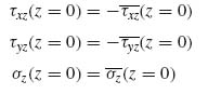
Note that a minus sign is needed in front of the shear stresses on the right-hand side to account for the orientation of the coordinate systems in Figure 9.14. As a result of Equations (9.64), the unknown functions f(y) and g(y) have to be the same for both flange and skin. In addition, the coefficients A1, B1, etc. for the skin, corresponding to the coefficients present in Equations (9.44b), (9.45b), (9.49), (9.51) and (9.54) for the flange, are also determined from Equations (9.64).
In order to determine the unknown functions f(y) and g(y), the principle of minimum complementary energy (see Section 5.4) is invoked. This means that the quantity
must be minimized. Underscores denote vectors and matrices. Overbars, as already mentioned, denote skin quantities. Specifically,
![]()
and S was given in Equation (9.55) above.
The last term of Equation (9.65) is the work term. It consists of the tractions T multiplying the prescribed displacements u*.
The stress expressions already determined are used to substitute in Equation (9.65). The x and z integrations can be carried out without difficulty because they only involve either powers or sines and cosines of the variables. Thus, after x and z integration, an expression for the energy is obtained in the form
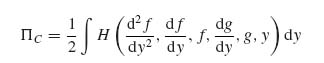
The problem has thus been recast as one in which the functions f(y) and g(y) must be determined such that the integral in the right-hand side of Equation (9.66) is minimized. This can be done by using the calculus of variations [15]. The general form of the Euler equations for f and g is as follows:
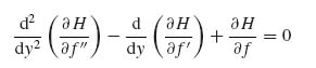
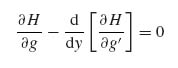
Using the detailed expression of H to substitute in Equations (9.67) and (9.68) yields the two equations:
where R1–R7 are constants obtained from the x and z integrations implied by Equation (9.65) and can be found in [2].
It should be noted that Equations (9.67a) and (9.68a) are given as homogeneous equations. In fact, Equations (9.67a) and (9.68a) would yield a nonhomogeneous term, that is, the right-hand side of Equations (9.67a) and (9.68a) is, in general, nonzero. However, it can be shown [2] that the nonhomogeneous terms affect only the far-field behaviour of the stresses which is already incorporated in the stress expressions. So the nonhomogeneous part of the solution can be neglected without loss of generality.
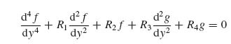
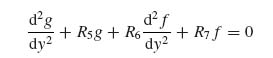
The two Equations (9.67a) and (9.68a) are coupled ordinary differential equations with constant coefficients. Following standard procedures the solutions can be written using exponentials:
where the exponents φi are solutions to
There are, in general, six solutions to Equation (9.71), but because only even powers of φ are present, they will appear in positive and negative pairs. Positive values of φ (or φ values with positive real parts) imply that f and g grow indefinitely as y increases, which implies that the interlaminar stresses containing f and g and their derivatives will tend to infinity for large values of y. This, however, is unacceptable as the interlaminar stresses must go to zero for large values of y in order for the far-field solution to be recovered. This is the reason for the negative exponents in Equations (9.69) and (9.70). It is assumed that φ1, φ2 and φ3 correspond to the positive solutions of Equation (9.71) (or those with positive real parts) so that the expressions for f and g are in terms of decaying exponentials.
One additional comment pertaining to the limits of the integral in Equation (9.66) is in order. The lower limit is zero, the edge of the flange. The upper limit is any large but finite value of y, corresponding to a point where the far-field stresses are recovered. Of course, if the flange of the stiffener is very narrow, the negative exponentials in Equations (9.69) and (9.70) have not died out and those two expressions for f and g must be modified to include the remaining three φ solutions of (9.71) which correspond to increasing exponentials. As already alluded to, some of the solutions to Equation (9.71) may be complex, in which case, expressions (9.69) and (9.70) will include complex conjugates.
Proceeding with the solution to the system of the two Equations (9.67a) and (9.68a) it can be shown that
(9.72) 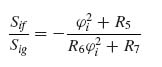
which relates the coefficients in function f(y) to those in function g(y).
At this point in the solution, the following unknowns remain: S1f, S2f, S3f, B1 and C2 in the flange and ![]() 2 in the skin. To determine these, the remaining boundary conditions, namely that the flange edge is stress free, are imposed:
2 in the skin. To determine these, the remaining boundary conditions, namely that the flange edge is stress free, are imposed:
(9.73) 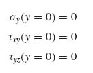
which, using the expressions for the stresses and the solution to the governing equations for f and g, become
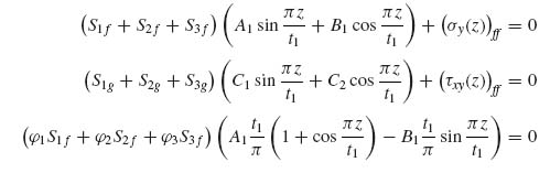
Since Equations (9.74a–c) involve sines and cosines of the variable z, the far-field stresses (σy(z))ff and (τxy(z))ff are expanded in Fourier series and the first terms used to match the corresponding terms in Equations (9.74a–c). This introduces an additional approximation in the solution, but the results are still accurate enough to give reliable trends of the behaviour.
Once Equations (9.74a–c) are solved, all unknown constants in the stress expressions are determined except for ![]() 2 in the skin. This, again, is determined by energy minimization
2 in the skin. This, again, is determined by energy minimization

which yields a linear equation for ![]() 2. The details of the algebra can be found in [2].
2. The details of the algebra can be found in [2].
The predictions of the method presented here have been compared with finite element results [2-4] and shown to be in good to excellent agreement. Discrepancies and reasons for them are discussed in the references. In what follows, the solution will be used to generate trend curves and discuss the implications for design.
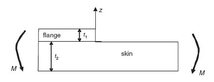
To gain insight on how different parameters affect the tendency of a stiffener to peel away from a skin, a typical flange and skin portion of a stiffened panel is isolated in Figure 9.15. The applied loading is simplified to an applied moment M. This could be the result of bending loads (e.g. pressure) applied on the panel or even post-buckling where local in-plane axial and/or shear loads are neglected.
Figure 9.15 Skin–flange configuration under bending load
The basic material properties are as follows:
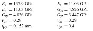
Note that, for this type of problem where out-of-plane stresses are involved, the out-of-plane stiffness properties Ez, Gxz, Gyz, νxz and νyz of the basic ply are also needed.
For the first set of results, the skin and flange layup are assumed to be the same [45/–45/–45/45]n in order to eliminate stiffness mismatch due to differences in moduli in the flange and skin. Only the thicknesses of skin and flange are allowed to vary by specifying different values of n. The normal stress σz at the interface between the skin and flange is plotted against distance from the flange edge for different values of the ratio t1/t2 in Figure 9.16. It is normalized with the maximum tensile value of σy at the far field which is given by
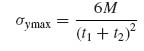
with M the applied moment per unit of stiffener length.
Figure 9.16 Normal stress as a function of distance from flange end for various thickness ratios
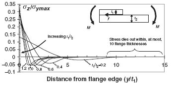
As expected from the qualitative discussion in association with Figure 9.11 at the beginning of this section, the normal stress has a maximum value at the edge of the flange and then reduces rapidly to negative values and decays to zero. The higher the value of t1/t2 the more rapidly the stress decays to zero. The distance over which the normal stress decays to zero does not exceed 10 flange thicknesses as is shown in Figure 9.16.
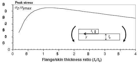
It is also apparent from Figure 9.16 that starting from low t1/t2 values and going up, the peak stress at the flange edge increases. However, this trend is not monotonic. As is shown in Figure 9.17, for the same skin and flange layups as in Figure 9.16, the highest peaks are reached for t1/t2 values between 1 and 1.5 and then decrease again. This means that flange thicknesses close to the skin thickness should be avoided because they maximize the normal stresses at the interface.
Figure 9.17 Peak normal stress at the flange edge as a function of flange to skin thickness ratio
The discussion so far has attempted to isolate the effect of geometry by keeping the layup of the flange and skin the same. Now, the thicknesses of the flange and skin are fixed to the same value and the layup is varied. This is shown in Figure 9.18 where the case of [45/–45]s flange and skin is compared with the extreme case of an all 0° flange, [04], on an all 90° skin, [904]. This is the most extreme case because it has the largest stiffness mismatch between the skin and flange. Note that the 0 direction is taken to be parallel to the y axis for this example.
Figure 9.18 Dependence of interface normal stress on layup
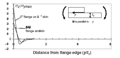
The [04] flange on [904] skin has a peak normal stress that is twice as high as the peak stress when skin and flange are both [45/–45]s. And, because the peak value is higher, the stress decays to zero faster than in the case of [45/–45]s skin and flange. An attempt to combine the effect of layup and geometry is shown in Figure 9.19 where the peak stress is plotted as a function of the ratio t1/t2 for the two layups of Figure 9.18.
Figure 9.19 Peak normal stress as a function of thickness ratio (t1/t2) for two different layup configurations
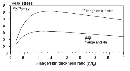
Again, the highest peaks occur for t1/t2 ratios between 1 and 1.5. In addition, the 0° flange on 90° skin has much higher peaks (as much as two times higher) than a situation where the flange and skin have the same layup. Only for t1/t2 values lower than 0.3 do the two cases approach each other but even for t1/t2 = 0.2 the 0° flange on 90° skin has 40% higher peak normal stress at the flange edge.
The results presented in Figures 9.16–9.19 were based on a case where only a bending moment M was applied. Similar results are obtained for other types of loading (but see Exercise 9.5 for some important differences). The trends can be summarized into the following recommendations or guidelines for design:
These implications for design rely heavily on the peak value of the normal stress at the flange–skin interface. This value occurs at the edge of the flange. It is important to note that the exact value at that location is not easy to determine. While the method presented in this section gives a well-defined value for the peak stress, the approximations and assumptions made in the derivation suggest that it may not be sufficiently accurate. On the other hand, finite element solutions show that the value at the edge itself is a function of the mesh size. In general, the finer the mesh near the flange edge, the higher the value. This is a well-known problem associated with free edges in composite materials [16, 17], and displacement-based formulations have difficulty in obtaining accurate stresses because the stress-free boundary condition is implemented in an average sense [17, 18]. In addition, exact anisotropic elasticity solutions for simple laminates [19, 20] have shown that, indeed, the stresses are, in general, singular at the free edge. However, in most cases, the strength of the singularity is so low that it becomes significant over a range equivalent to a few fibre diameters. In such a case, the main assumption of homogeneity in the elasticity solution breaks down and the two different constituents, fibre and matrix, must be modelled separately. As a result, the elasticity solution is no more reliable than finite element solutions or the approach presented in this section.
From a design perspective, any method that gives accurate stresses near the free edge of the flange (but not necessarily the flange edge itself) can be used to differentiate between design candidates. Configurations with higher peak values at the edge are expected to have inferior performance. Predicting the exact load at which a delamination will start requires the use of some failure criterion [13, 14] and some test results to adjust any discrepancies between the value predicted at the edge by the analysis method used and the actual test value.
The design guidelines presented in this section can now be used to revisit and upgrade the design of the stiffener cross-section that was last reviewed in Figure 8.36. The revised design is shown in Figure 9.20. The two main differences from Figure 8.36 are the stepped flange next to the skin where plies are dropped with the distance between drops at least 10 times the height of the dropped ply (or plies if more than one ply is dropped at the same location) and the requirement that the skin and flange thicknesses be different (tflange/tskin < 1 or >1.5) with layups that are, if possible, multiples of the same base layup to keep the respective in-plane stiffnesses as close as possible.
Figure 9.20 Stiffener cross-section design incorporating guidelines from this section
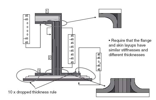
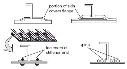
It is recognized, of course, that by using a stepped flange next to the skin the manufacturing cost increases significantly. A tradeoff between the increased cost associated with the stepped flange and the improvement in performance (and thus decreased weight) is necessary in such cases. Alternatives to the stepped flange are shown in Figure 9.21. While they all improve the performance of the skin-stiffened panel, they all carry a significant cost penalty with them.
Figure 9.21 Different options for delaying skin–stiffener separation
9.3 Additional Considerations for Stiffened Panels
9.3.1 ‘Pinching’ of Skin
With shear loads present, the skin between stiffeners goes into diagonal tension (see Section 7.2). Resolving the shear load in biaxial tension and compression as was done in Section 7.2 results in the situation shown in Figure 9.22. Only the base flanges of the stiffeners are shown in this figure for clarity.
Figure 9.22 Local tension and compression regions in skin under shear
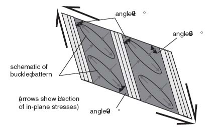
Of particular importance during testing of such configurations are the compression regions at the top left and bottom right of each bay (the term bay here refers to the section between stiffeners). Locally there, an originally rectangular piece of skin deforms such that the angle at the corners of interest is less than 90° (Figure 9.22). If the applied load is sufficiently high, this can cause the skin to fail in compression. This ‘pinching’ phenomenon is more pronounced on components isolated from the surrounding structure during, for example, testing of individual panels. In a complete structure such as a fuselage or wing skin, the conditions at the edges of the panel in Figure 9.22 are different from when it is isolated in a test fixture and the compliance of the adjacent structure relieves this phenomenon.
Pinching of skin at the corners may lead to a premature failure when testing in the laboratory. This can happen even before the skin buckles and it can be exacerbated by local eccentricities that may introduce additional bending moments in the region where the skin is under compression. For this reason special fixtures and specimen geometries have been designed to eliminate this problem [21].
9.3.2 Co-curing versus Bonding versus Fastening
The discussion in this book has mostly been confined to generating designs that meet the loads at low weights. Other than Chapter 2 and Sections 5.1.1, 5.1.2, 9.2.2 and 13.4, little attention has been paid to the cost associated with some of the designs that result from the approaches presented. The subject of skin-stiffened structure is ideal for bringing up some additional considerations relative to assembly cost and how different concepts can be traded with cost as an additional driver.
There are three major ways in which a stiffened panel can be assembled: (a) co-curing, (b) bonding and (c) fastening. There are variations or combinations of those such as co-bonding (where one or both of skin and stiffeners are staged and then cured with adhesive present), bonding and fastening, but these three major options are a good starting point for cost tradeoffs.
To discuss these approaches some basic aspects and experience-based conclusions should be laid down first:
In co-curing, the skin and stiffeners are cured at the same time. This requires detailed (and costly) tooling to accurately locate the stiffeners during cure and to ensure uniform pressure everywhere. So the nonrecurring cost associated with tooling is relatively high. The recurring cost (labour hours) per unit weight is relatively low according to item (1) above. On the other hand, the risk of something going wrong during cure of the combined skin and stiffeners is relatively high, which, according to item (5) above, adds to the cost.
In a bonded configuration, skin and stiffeners are made separately which minimizes the risk. But bonding requires the extra assembly step of skin and stiffeners thus adding to the cost. In addition, there are currently no reliable consistent nondestructive inspection methods to verify that the bond is everywhere effective and meets minimum strength requirements. This means that additional process steps ensuring proper surface preparation of the surfaces to be bonded, full coverage with adhesive, cleanliness and avoidance of contamination, etc. have to be in place to guarantee a good bondline. This adds to the cost. In some cases, to protect against defective bondlines that were missed during fabrication and inspection, it is required to demonstrate that the structure can meet limit load with a significant portion of the bondline ineffective, which adds to the weight of the structure.
Fastening of the stiffeners to the skin eliminates the problems associated with bonding and improves the post-buckling performance. However, the extra assembly time associated with fastening is a significant cost increase. In addition, the use of fasteners typically increases the weight.
It can be seen from the previous discussion that each of the three approaches has advantages and disadvantages, and deciding which approach to follow is a function of the amount of risk to be undertaken and which process steps a particular facility is more comfortable with and more efficient in. It is possible, for example, if the assembly process steps are streamlined and automated, that the cost associated with them is only a small fraction of the total and can lead to overall cost savings compared with a co-cured configuration [22].
Exercises
9.1 Assume that the stiffener used in the application in Section 8.5.3.1 is to be used on a square skin panel of dimensions 508 × 508 mm loaded in compression. The skin layup is [45/–45]s (same material as the stiffener). Determine the largest stiffener spacing (and thus the spacing that minimizes the number of stiffeners and therefore the fabrication cost) such that the overall buckling load equals the buckling load of the skin portion between the stiffeners.
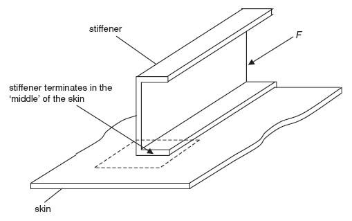
9.2 Consider the stiffener terminating somewhere on a skin as shown in the figure.
Further isolating the flange and skin portions included in the dashed rectangle above and viewing them from the side (enlarged):
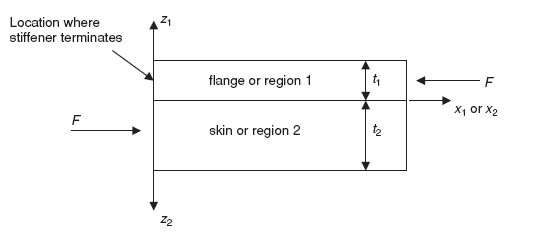
Note the following:
It is assumed that far from the terminating flange edge (i.e. for high values of x1) the classical laminated-plate theory is recovered according to which the average stress in the flange σ1 is given by
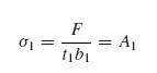
where b1 is the flange width.
It is now assumed that the normal stress σx1 in the flange is given by the following expression:
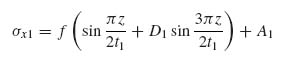
where f is an unknown function of x1 and D1 is an unknown constant.
Note that this expression can be viewed as consisting of the first few terms of a Fourier series. The requirement, of course, is that f, for large x1, tends to zero so σx1 → A1 away from the flange termination.
Use the equilibrium equations to determine the stresses τxz1 and σz1 (all other stresses are zero or close to zero in the flange). To do this you will also need to make sure that τxz1 = 0 and σz1 = 0 at the top of the flange. Also, write the corresponding stress expressions for region 2 (by analogy with region 1).
Require that τxz and σz are continuous at the flange–skin interface (i.e. the value of τxz obtained at the flange–skin interface coming from the flange equals the value of τxz obtained at the same location coming from the skin, and similarly for σz) and obtain the values of D1 and D2. (Watch out for the definition of the coordinate systems and the z direction.)
9.3 Continuing from Exercise 9.2, the function f is still unknown. To determine it you need to minimize the energy in the flange–skin system. The energy has the form
![]()
where the internal potential energy U is the sum of U1 and U2 and W is the external work. It turns out that W does not contribute to the solution so neglect it.
Now U1 is given by
![]()
where all quantities in the right-hand side should have an additional subscript 1 to denote the flange (omitted here for simplicity) and the quantities Sij are compliances (obtained from inverting the stiffness matrix for the entire flange).
The y integration only yields a constant b1, the width of the flange, since there is no dependence on y.
Without substituting for D1 (and D2) use your expressions for the stresses obtained in Exercise 9.2 and perform the z integrations in the expression for U1. Note that, because these involve sines and cosines, quite a few of the integrals are zero and you can derive simple expressions for those that are not.
Write the analogous expression for U2 and perform the z integration. Note that the y integration in the skin will also yield a constant multiplier of b1 because we are assuming that the skin–flange portion we have isolated for analysis is of width b1 both for the flange and the skin.
If you substitute in the expression for Π = U1 + U2 you will now have a long integral with respect to x only (y and z integrations already performed) which will be a function of f and its first two derivatives.
9.4 Continuing from Exercise 9.3, using the calculus of variations write down the Euler equation for this problem and derive the governing equation for f so that the energy is minimized. Write the governing equation in the form
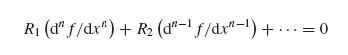
Start with R1 with the highest derivative of f, and neglect the constant term (because it does not contribute to the solution). Write down the expressions for R1, R2, ….
Solve the equation obtained writing down the solution in the form
![]()
Also write down the expression for mi.
9.5 (Continuing from Exercise 9.4) At this point, the fact that none of the stresses can increase with increasing x is invoked and only exponentials with negative real parts are used. In addition, the boundary conditions that require τxz1 = 0 and σx1 = 0 at x = 0 are invoked (the second one approximately only) and the constants C1, C2, … are determined. After that is done, one notices that at x1 = 0 at the flange–skin interface, the interlaminar shear stresses τxz1 and τxz2 are zero and only the normal stress σz1 or σz2 is nonzero. Therefore, the only stress that contributes to delamination is σz1 (or σz2 which is the same at the flange–skin interface by stress continuity).
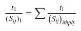
Substituting in the stress expressions and evaluating σz1 at x = z = 0 shows that
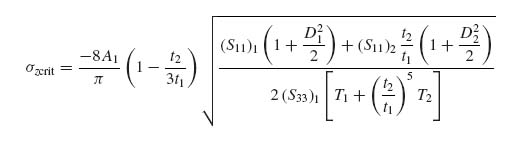
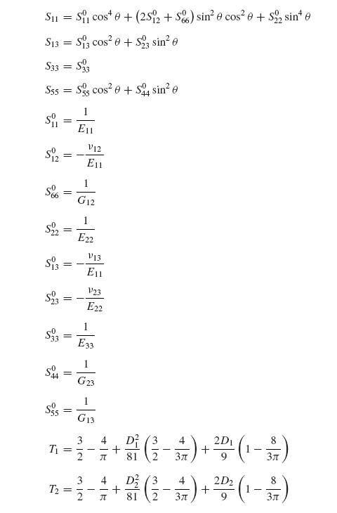
where the compliances for each laminate (flange or skin) can be obtained by averaging the compliances over all plies (springs in series):
with an analogous expression for region 2, and the compliances for each ply of orientation θ are given by the following expressions where quantities with superscript 0 refer to a 0° ply of the material being used:
A material is made available with the following properties:
It is also given that the skin at the location of interest has the following layup: [45/–45/0/90]s4.
9.6 (a) If the skin is not to exceed 4500 $ μs, determine the value of F that barely fails the skin. (b) Assume that the flange is made from one of the three layups: [0/90]sn or [45/–45]sm or [45/–45/0/90]s p. Select a value of n, m and p and plot the value of σzcrit as a function of t2/t1. Which value(s) of t2/t1 would you recommend to use in this case and why? (c) Use your results in (a) and (b) to select the lightest flange layup you should use.
References
[1] Megson, T.H.G., Aircraft Structures for Engineering Students, Elsevier, Oxford, UK, 2007, Chapter 3.
[2] Kassapoglou, C., Stress Determination at Skin-Stiffener Interfaces of Composite Stiffened Panels under Generalized Loading, Journal of Reinforced Plastics and Composites, 13, 1555–1572 (1994).
[3] Kassapoglou, C., Calculation of Stresses at Skin-Stiffener Interfaces of Composite Stiffened Panels under Shear Loads, International Journal of Solids and Structures, 30, 1491–1503 (1993).
[4] Kassapoglou, C. and DiNicola, A.J., Efficient Stress Solutions at Skin Stiffener Interfaces of Composite Stiffened Panels, AIAA Journal, 30, 1833–1839 (1992).
[5] Hyer, M.W. and Cohen, D., Calculation of Stresses and Forces between the Skin and Stiffener in Composite Panels, AIAA Paper 87-0731, 28th SDM Conference, Monterey, CA, April 1987.
[6] Cohen, D. and Hyer, M.W., Influence of Geometric Non-linearities on Skin-Stiffener Interface Stresses, AIAA Paper 88-2217, 29th SDM Conference, Williamsburg, VA, April 1988.
[7] Volpert, Y. and Gottesman, T., Skin-Stiffener Interface Stresses in Tapered Composite Panel, Composite Structures, 33, 1–6 (1995).
[8] Baker, D.J. and Kassapoglou, C., Post Buckled Composite Panels for Helicopter Fuselages: Design, Analysis, Fabrication and Testing. Presented at the American Helicopter Society International Structures Specialists' Meeting, Hampton Roads Chapter, Structures Specialists Meeting, Williamsburg, VA, 30 October–1 November 2001.
[9] Wiggenraad, J.F.M. and Bauld, N.R., Global/Local Interlaminar Stress Analysis of a Grid-Stiffened Composite Panel, Journal of Reinforced Plastics and Composites, 12, 237–253 (1993).
[10] Minguet, P.J. and O'Brien, T.K., Analysis of Test Methods for Characterizing Skin/Stringer Debonding Failures in Reinforced Composite Panels, in Composite Materials: Testing and Design ASTM STP 1274, R.B. Deo and C.R. Saff (eds), American Society for Testing and Materials, Philadelphia, PA, 1996, pp 105–124.
[11] Wang, J.T. and Raju, I.S., Strain Energy Release Rate Formulae for Skin-Stiffener Debond Modeled with Plate Elements, Engineering Fracture Mechanics, 54, 211–228 (1996).
[12] Wang, J.T., Raju, I.S. and Sleight, D.W., Composite Skin-Stiffener Debond Analyses, Using Fracture Mechanics Approach with Shell Elements, Composites Engineering, 5, 277–296 (1995).
[13] Brewer, J.C. and Lagace, P.A., Quadratic Stress Criterion for Initiation of Delamination, Journal of Composite Materials, 22, 1141–1155 (1988).
[14] Fenske, M.T., and Vizzini, A.J., The Inclusion of In-Plane Stresses in Delamination Criteria, Journal of Composite Materials, 35, 1325–1342 (2001).
[15] Hildebrandt, F.B., Advanced Calculus for Applications, Prentice Hall, Englewood Cliffs, NJ, 1976, Section 7.8.
[16] Wang, A.S.D. and Crossman, F.W., Some New Results on Edge Effect in Symmetric Composite Laminates, Journal of Composite Materials, 11, 92–106 (1977).
[17] Bauld, N.R., Goree, J.G. and Tzeng, L.-S., A Comparison of Finite-Difference and Finite Element Methods for Calculating Free Edge Stresses in Composites, Composites and Structures, 20, 897–914 (1985).
[18] Spilker, R.L. and Chou, S.C., Edge Effects in Symmetric Composite Laminates: Importance of Satisfying the Traction-Free-Edge Condition, Journal of Composite Materials, 14, 2–20 (1980).
[19] Wang, S.S. and Choi, I., Boundary-Layer Effects in Composite Laminates, Part I – Free Edge Stress Solutions and Basic Characteristics, ASME Transactions Applied Mechanics, 49, 541–548 (1982).
[20] Wang, S.S. and Choi, I., Boundary-Layer Effects in Composite Laminates, Part II – Free Edge Stress Solutions and Basic Characteristics, ASME Transactions Applied Mechanics, 49, 549–560 (1982).
[21] Farley, G.L. and Baker, D.J., In-Plane Shear Test of Thin Panels, Experimental Mechanics, 23, 81–88 (1983).
[22] Apostolopoulos, P. and Kassapoglou, C., Cost Minimization of Composite Laminated Structures – Optimum Part Size as a Function of Learning Curve Effects and Assembly, Journal of Composite Materials, 36(4), 501–518 (2002).