2

Cost of Composites: a Qualitative Discussion

Considering that cost is the most important aspect of an airframe structure (along with the weight), one would expect it to be among the best defined, most studied and most optimized quantities in a design. Unfortunately, it remains one of the least understood and ill-defined aspects of a structure. There are many reasons for this inconsistency, some of which are: (a) cost data for different fabrication processes and types of parts are proprietary and only indirect or comparative values are usually released; (b) there seems to be no well-defined reliable method to relate design properties such as geometry and complexity to the cost of the resulting structure; (c) different companies have different methods of bookkeeping the cost and it is hard to make comparisons without knowing these differences (e.g. the cost of the autoclave can be apportioned to the number of parts being cured at any given time or it may be accounted for as an overhead cost, included in the total overhead cost structure of the entire factory); (d) learning curve effects, which may or may not be included in the cost figures reported, tend to confuse the situation especially since different companies use different production run sizes in their calculations.

These issues are common to all types of manufacturing technologies and not just the aerospace sector. In the case of composites, the situation is further complicated by the relative novelty of the materials and processes being used, the constant emergence of new processes or variations thereof that alter the cost structure and the high nonrecurring cost associated with switching to the new processes that, usually, acts as a deterrent towards making the switch.

The discussion in this chapter attempts to bring up some of the cost considerations that may affect a design. This discussion is by no means exhaustive; in fact, it is limited by the lack of extensive data and generic but accurate cost models. It serves mainly to alert or sensitize a designer to several issues that affect the cost. These issues, when appropriately accounted for, may lead to a robust design that minimizes the weight and is cost competitive with the alternatives.

The emphasis is placed on recurring and nonrecurring costs. The recurring cost is the cost that is incurred every time a part is fabricated. The nonrecurring cost is the cost that is incurred once during the fabrication run.

2.1 Recurring Cost

The recurring cost includes the raw material cost (including scrap) for fabricating a specific part, the labour hours spent in fabricating the part and cost of attaching it to the rest of the structure. The recurring cost is hard to quantify, especially for complex parts. There is no single analytical model that relates specific final part attributes such as geometry, weight, volume, area or complexity to the cost of each process step and through the summation over all process steps to the total recurring cost. One of the reasons for these difficulties and, as a result, the multitude of cost models that have been proposed with varying degrees of accuracy and none of them all-encompassing, is the definition of complexity. One of the most rigorous and promising attempts to define complexity and its effect on the recurring cost of composite parts was by Gutowski et al. [1, 2].

For the case of hand layup, averaging over a large quantity of parts of varying complexity ranging from simple flat laminates to compound curvature parts with co-cured stiffeners, the fraction of total cost taken up by the different process steps is shown in Figure 2.1 (taken from Reference 3).

It can be seen from Figure 2.1 that, by far, the costliest steps are locating the plies into the mould (42%) and assembling to the adjacent structure (29%). Over the years, cost-cutting and optimization efforts have concentrated mostly on these two process steps. This is the reason for introducing automation. Robots, used for example in automated tape layup, take the cut plies and locate them automatically in the mould, greatly reducing the cost associated with that process step, improving the accuracy and reducing or eliminating human error, thereby increasing consistency and quality. Since assembly accounts for about one-third of the total cost, increasing the amount of co-curing where various components are cured at the same time reduces drastically the assembly cost. An example of this integration is shown in Figure 2.2.

These improvements as well as others associated with other process steps such as automated cutting (using lasers or water jets), trimming and drilling (using numerically controlled equipment) have further reduced the cost and improved quality by reducing the human involvement in the process. Hand layup and its automated or semi-automated variations can be used to fabricate just about any piece of airframe structure. An example of a complex part with compound curvature and parts intersecting in different directions is shown in Figure 2.3.

Further improvements have been brought to bear by taking advantage of the experience acquired in the textile industry. By working with fibres alone, several automated techniques such as knitting, weaving, braiding and stitching can be used to create a preform, which is then injected with resin. This is the resin transfer moulding (RTM) process. The raw material cost can be less than half the raw material cost of preimpregnated material (prepreg) used in hand layup or automated tape layup because the impregnation step needed to create the prepreg used in those processes is eliminated. On the other hand, ensuring that the resin fully wets all fibres everywhere in the part and that the resin content is uniform and equal to the desired resin content can be hard for complex parts and may require special tooling, complex design of injection and overflow ports and use of high pressure. It is not uncommon, for complex RTM parts to have 10–15% less strength (especially in compression and shear) than their equivalent prepreg parts due to reduced resin content. Another problem with matched metal moulding RTM is the high nonrecurring cost associated with the fabrication of the moulds. For this reason, variations of the RTM process such as vacuum-assisted RTM (VARTM) where one of the tools is replaced by a flexible caul plate whose cost is much lower than an equivalent matched metal mould or resin film infusion (RFI) where the resin is drawn into dry fibre preforms from a pool or film located under it and/or from staged plies that already have resin in them, have been used successfully in several applications (Figure 2.4). Finally, due to the fact that the process operates with resin and fibres separately, the high amounts of scrap associated with hand layup can be significantly reduced.

Introduction of more automation led to the development of automated fibre or tow placement. This was a result of trying to improve filament winding (see below). Robotic heads can each dispense material as narrow as 3 mm and as wide as 100 mm by manipulating individual strips (or tows) each 3 mm wide. Tows are individually controlled so the amount of material laid down in the mould can vary in real time. Starting and stopping individual tows also allows the creation of cutouts ‘on the fly’. The robotic head can move in a straight line at very high rates (as high as 30 m/min). This makes automated fibre placement an ideal process for laying material down to create parts with large surface area and small variations in thickness or with a limited number of cutouts. For maximum efficiency, structural details (e.g. cutouts) that require starting and stopping the machine or cutting material while laying it down should be avoided. Material scrap is very low. Convex as well as concave tools can be used since the machine does not rely on constant fibre tension, as in filament winding, to lay the material down. There are limitations with the process associated with the accuracy of starting and stopping when material is laid down at high rates and the size and shape of the tool when concave tools are used (in order to avoid interference of the robotic head with the tool). The ability to steer fibres on prescribed paths (Figure 2.5) can also be used as an advantage by transferring the loads efficiently across the part. This results in laminates where stiffness and strength are a function of location and provides an added means for optimization [4, 5].

Automated fibre placement is most efficient when making large parts. Parts such as stringers, fittings, small frames that do not have at least one sizeable side where the advantage of the high lay-down rate of material by the robotic head can be brought to bear, are hard to make and/or not cost competitive. In addition, skins with large amounts of taper and number of cutouts may also not be amenable to this process.

In addition to the above processes that apply to almost any type of part (with some exceptions already mentioned for automated fibre placement) specialized processes that are very efficient for the fabrication of specific part types or classes of parts have been developed. The most common of these are filament winding, pultrusion and press moulding using long discontinuous fibres and sheet moulding compounds.

Filament winding, as already mentioned, is the precursor to advanced fibre or tow placement. It is used to make pressure vessels and parts that can be wound on a convex mandrel. The use of a convex mandrel is necessary in order to maintain tension on the filaments being wound. The filaments are drawn from a spool without resin and are driven through a resin bath before they are wound around the mandrel. Due to the fact that tension must be maintained on the filaments, their paths can only be geodetic paths on the surface of the part being woven. This means that, for a cylindrical part, if the direction parallel to the cylinder axis is denoted as the zero direction, winding angles between 15° and 30° are hard to maintain (filaments tend to slide) and angles less than 15° cannot be wound at all. Thus, for a cylindrical part with conical closeouts at its ends, it is impossible to include 0° fibres using filament winding. 0° plies can be added by hand if necessary at a significant increase in cost. Since the material can be dispensed at high rates, filament winding is an efficient and low-cost process. In addition, fibres and matrix are used separately and the raw material cost is low. Material scrap is very low.

Pultrusion is a process where fibres are pulled through a resin bath and then through a heated die that gives the final shape. It is used for making long constant-cross-section parts such as stringers and stiffeners. Large cross-sections, measuring more than 25 × 25 cm are hard to make. Also, because fibres are pulled, if the pulling direction is denoted by 0°, it is not possible to obtain layups with angles greater than 45° (or more negative than –45°). Some recent attempts have shown it is possible to obtain longitudinal structures with some taper. The process is very low cost. Long parts can be made and then cut at the desired length. Material scrap is minimal.

With press moulding it is possible to create small three-dimensional parts such as fittings. Typically, composite fittings made with hand layup or RTM without stitching suffer from low out-of-plane strength. There is at least one plane without any fibres crossing it and thus only the resin provides strength perpendicular to that plane. Since the resin strength is very low, the overall performance of the fitting is compromised. This is the reason some RTM parts are stitched. Press moulding (Figure 2.6) provides an alternative with improved out-of-plane properties. The out-of-plane properties are not as good as those of a stitched RTM structure, but better than hand laid-up parts and the low cost of the process makes them very attractive for certain applications. The raw material is essentially a slurry of randomly oriented long discontinuous fibres in the form of chips. High pressure applied during cure forces the chips to completely cover the tool cavity. Their random orientation is, for the most part, maintained. As a result, there are chips in every direction with fibres providing extra strength. Besides three-dimensional fittings, the process is also very efficient and reliable for making clips and shear ties. Material scrap is minimal. The size of the parts to be made is limited by the press size and the tool cost. If there are enough parts to be made, the high tooling cost is offset by the low recurring cost.

There are other fabrication methods or variations within a fabrication process that specialize in certain types of parts and/or part sizes. The ones mentioned above are the most representative. There is one more aspect that should be mentioned briefly; the effect of learning curves. Each fabrication method has its own learning curve which is specific to the process, the factory and equipment used and the skill level of the personnel involved. The learning curve describes how the recurring cost for making the same part multiple times decreases as a function of the number of parts. It reflects the fact that the process is streamlined and people find more efficient ways to do the same task. Learning curves are important when comparing alternative fabrication processes. A process with a steep learning curve can start with a high unit cost but, after a sufficiently large number of parts, can yield unit costs much lower than another process, which starts with lower unit cost, but has a shallower learning curve. As a result, the first process may result in lower average cost (total cost over all units divided by the number of units) than the first.

As a rule, fabrication processes with little or no automation have steeper learning curves and start with higher unit cost. This is because an automated process has fixed throughput rates while human labour can be streamlined and become more efficient over time as the skills of the people involved improve and ways of speeding up some of the process steps used in making the same part are found. The hand layup process would fall in this category with, typically, an 85% learning curve. An 85% learning curve means that the cost of unit 2n is 85% of the cost of unit n. Fabrication processes involving a lot of automation have shallower learning curves and start at lower unit cost. One such example is the automated fibre/tow placement process with, typically, a 92% learning curve. A discussion of some of these effects and the associated tradeoffs can be found in Reference 3.

An example comparing a labour intensive process with 85% learning curve and cost of unit one 40% higher than an automated fabrication process with 92% learning curve is given here to highlight some of the issues that are part of the design phase, in particular at early stages when the fabrication process or processes have not been finalized yet.

Assuming identical units, the cost of unit n, C(n), is assumed to be given by a power law:

(2.1)

where C(1) is the cost of unit 1 and r is an exponent that is a function of the fabrication process, factory capabilities, personnel skill, etc.

If p% is the learning curve corresponding to the specific process, then

(2.2)

Using Equation (2.1) to substitute in Equation (2.2) and solving for r, it can be shown that,

(2.3)

For our example, with process A having pA = 0.85 and process B having pB = 0.92, substituting in Equation (2.3) gives rA = 0.2345 and rB = 0.1203. If the cost of unit 1 of process B is normalized to 1, CB(1) = 1, then the cost of unit 1 of process A will be 1.4, based on our assumption stated earlier, so CA(1) = 1.4. Putting it all together,

(2.4)

(2.5)

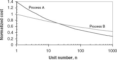
The cost as a function of n for each of the two processes can now be plotted in Figure 2.7. A logarithmic scale is used on the x axis to better show the differences between the two curves.

It can be seen from Figure 2.7 that a little after the 20th part, the unit cost of process A becomes less than that of process B suggesting that for sufficiently large runs, process A may be competitive with process B. To investigate this further, the average cost over a production run of N units is needed. If N is large enough, the average cost can be accurately approximated by:

(2.6)

and using Equation (2.1),

(2.7)

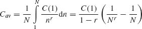
Note that to derive Equation (2.7) the summation was approximated by an integral. This gives accurate results for N > 30. For smaller production runs (N < 30) the summation in Equation (2.6) should be used. Equation (2.7) is used to determine the average cost for Process A and Process B as a function of the size of the production run N. The results are shown in Figure 2.8.

As can be seen from Figure 2.8, Process B, with automation, has lower average cost as long as less than approximately 55 parts are made (N < 55). For N > 55, the steeper learning curve of Process A leads to lower average cost for that process. Based on these results, the less-automated process should be preferred for production runs with more than 50–60 parts. However, these results should be viewed only as preliminary, as additional factors that play a role were neglected in the above discussion. Some of these factors are briefly discussed below.

Process A, which has no automation, is prone to human errors. This means that: (a) the part consistency will vary more than in Process B; and (b) the quality and accuracy may not always be satisfactory requiring repairs or scrapping of parts.

In addition, process improvements, which the equations presented assume to be continuous and permanent, are not always possible. It is likely that after a certain number of parts, all possible improvements have been implemented. This would suggest that the learning curves typically reach a plateau after a while and the cost cannot be reduced below that plateau without major changes in the process (new equipment, new process steps, etc.). These drastic changes are more likely in automated processes where new equipment is developed regularly than in a nonautomated process. Therefore, while the conclusion that a less-automated process will give lower average cost over a sufficiently large production run is valid, in reality, it may only occur under very special circumstances favouring continuous process improvement, consistent high part quality and part accuracy, etc. In general, automated processes are preferred because of their quality, consistency and potential for continuous improvement.

The above is a very brief reference to some of the major composite fabrication processes. It serves to bring some aspects to the forefront as they relate to design decisions. More in-depth discussion of some of these processes and how they relate to the design of composite parts can be found in References 6 and 7.

2.2 Nonrecurring Cost

The main components of nonrecurring cost follow the phases of the development of a program and are the following.

Design. Typically divided in stages (e.g. conceptual, preliminary and detail) it is the phase of creating the geometry of the various parts and coming up with the material(s) and fabrication processes (see Sections 5.1.1 and 5.1.2 for a more detailed discussion). For composites it is more involved than for metals because it includes detailed definition of each ply in a layup (material, orientation, location of boundaries, etc.). The design of press-moulded parts would take less time than other fabrication processes as definition of the boundaries of each ply is not needed. The material under pressure fills the mould cavity and the concept of a ply is more loosely used.

Analysis. In parallel with the design effort, it determines applied loads for each part and comes up with the stacking sequence and geometry to meet the static and cyclic loads without failure and with minimum weight and cost. The multitude of failure modes specific to composites (delamination, matrix failure, fibre failure, etc.) makes this an involved process that may require special analytical tools and modelling approaches.

Tooling. This includes the design and fabrication of the entire tool string needed to produce the parts: moulds, assembly jigs and fixtures, etc. For composite parts cured in the autoclave, extra care must be exercised to account for thermal coefficient mismatch (when metal tools are used) and spring-back phenomena where parts removed from the tools after cure tend to deform slightly to release some residual thermal and cure stresses. Special (and expensive) metal alloys (e.g. invar) with low coefficients of thermal expansion can be used where dimensional tolerances are critical. Also careful planning of how heat is transmitted to the parts during cure for more uniform temperature distribution and curing is required. All these add to the cost, making tooling one of the biggest elements of the nonrecurring cost. In particular, if matched metal tooling is used, such as for RTM parts or press-moulded parts, the cost can be prohibitive for short production runs. In such cases an attempt is made to combine as many parts as possible in a single co-cured component. An idea of tool complexity when local details of a wing-skin are accommodated accurately is shown in Figure 2.9.

Nonrecurring fabrication. This does not include routine fabrication during production that is part of the recurring cost. It includes: (a) one-off parts made to toolproof the tooling concepts; (b) test specimens to verify analysis and design and provide the database needed to support design and analysis; and (c) producibility specimens to verify the fabrication approach and avoid surprises during production. This can be costly when large co-cured structures are involved with any of the processes already mentioned. It may take the form of a building-block approach where fabrication of subcomponents of the full co-cured structure is done first to check different tooling concepts and verify part quality. Once any problems (resin-rich, resin-poor areas, locations with insufficient degree of cure or pressure during cure, voids, local anomalies such as ‘pinched’ material, fibre misalignment), are resolved, more complex portions leading up to the full co-cured structure are fabricated to minimize the risk and verify the design.

Testing. During this phase, the specimens fabricated during the previous phase are tested. This includes the tests needed to verify analysis methods and provide missing information for various failure modes. This does not include testing needed for certification (see next item). If the design has opted for large co-cured structures to minimize recurring cost, the cost of testing can be very high since it, typically, involves testing of various subcomponents first and then testing the full co-cured component. Creating the right boundary conditions and applying the desired load combinations in complex components results in expensive tests.

Certification. This is one of the most expensive nonrecurring cost items. Proving that the structure will perform as required and providing relevant evidence to certifying agencies requires a combination of testing and analysis [8–10]. The associated test program can be extremely broad (and expensive). For this reason, a building-block approach is usually followed where tests of increasing complexity, but reduced in numbers follow simpler more numerous tests, each time building on the previous level in terms of information gained, increased confidence in the design performance and reduction of risk associated with the full-scale article. In a broad level description going from the simplest to the most complex: (a) material qualification where thousands of coupons with different layups are fabricated and tested under different applied loads and environmental conditions with and without damage to provide statistically meaningful values (see Sections 5.1.3–5.1.5) for strength and stiffness of the material and stacking sequences to be used; (b) element tests of specific structural details isolating failure modes or interactions; (c) subcomponent and component tests verifying how the elements come together and providing missing (or hard to otherwise accurately quantify) information on failure loads and modes; (d) full-scale test. Associated with each test level, analysis is used to reduce test data, bridge structural performance from one level to the next and justify the reduction of specimens at the next level of higher complexity. The tests include static and fatigue tests leading to the flight test program that is also part of the certification effort. When new fabrication methods are used, it is necessary to prove that they will generate parts of consistently high quality. This, sometimes, along with the investment in equipment purchasing and training, acts as a deterrent in switching from a proven method (e.g. hand layup) with high comfort level to a new method some aspects of which may not be well known (e.g. automated fibre placement).

The relative cost of each of the different phases described above is a strong function of the application, the fabrication process(es) selected and the size of the production run. It is, therefore, hard to create a generic pie chart that would show how the cost associated with each compares. In general, it can be said that certification tends to be most expensive followed by tooling, nonrecurring fabrication and testing.

2.3 Technology Selection

The discussion in the two previous sections shows that there is a wide variety of fabrication processes, each with its own advantages and disadvantages. Trading these and calculating the recurring and nonrecurring costs associated with each selection is paramount in coming up with the best choice. The problem becomes very complex when one considers large components such as the fuselage or the wing or entire aircraft. At this stage, it is useful to define the term ‘technology’ as referring to any combination of material, fabrication process and design concept. For example, graphite/epoxy skins using fibre placement would be one technology. Similarly, sandwich skins with a mixture of glass/epoxy and graphite/epoxy plies made using hand layup would be another technology.

In a large-scale application such as an entire aircraft, it is extremely important to determine the optimum technology mix, i.e. the combination of technologies that will minimize weight and cost. This can be quite complicated since different technologies are more efficient for different types of part. For example, fibre-placed skins might give the lowest weight and recurring cost, but assembling the stringers as a separate step (bonding or fastening) might make the resulting skin/stiffened structure less cost competitive. On the other hand, using resin transfer moulding to co-cure skin and stringers in one step might have lower overall recurring cost at a slight increase in weight (due to reduced strength and stiffness) and a significant increase in nonrecurring cost due to increased tooling cost. At the same time, fibre placement may require significant capital outlays to purchase automated fibre/tow placement machines. These expenditures require justification accounting for the size of the production run, availability of capital and the extent to which capital investments already made on the factory floor for other fabrication methods have been amortized or not.

These tradeoffs and final selection of optimum technology mix for the entire structure of an aircraft are done early in the design process and ‘lock in’ most of the cost of an entire program. For this reason it is imperative that the designer be able to perform these trades in order to come up with the ‘best alternatives’. As will be shown in this section these ‘best alternatives’ are a function of the amount of risk one is willing to take, the amount of investment available and the relative importance of recurring, nonrecurring cost and weight [11–14].

In order to make the discussion more tractable, the airframe (load-bearing structure of an aircraft) is divided into part families. These are families of parts that perform the same function, have approximately the same shapes, are made with the same material(s) and can be fabricated by the same manufacturing process. The simplest division into part families is shown in Table 2.1. In what follows the discussion will include metals for comparison purposes.

Table 2.1 Part families of an airframe

Part family	Description
Skins and covers	Two-dimensional parts with single curvature
Frames, bulkheads, beams, ribs, intercostals	Two-dimensional flat parts
Stringers, stiffeners, breakers	One-dimensional (long) parts
Fittings	Three-dimensional small parts connecting other parts
Decks and floors	Mostly flat parts
Doors and fairings	Parts with compound curvature
Miscellaneous	Seals, etc.

The technologies that can be used for each part family are then determined. This includes the material (metal or composite and, if composite, the type of composite), fabrication process (built-up sheet metal, automated fibre placement, resin transfer moulding, etc.) and design concept (e.g. stiffened skin versus sandwich). In addition, the applicability of each technology to each part family is determined. This means determining what portion in the part family can be made by the technology in question. Usually, as the complexity of the parts in a part family increases, a certain technology becomes less applicable. For example, small skins with large changes in thickness across their length and width cannot be made by fibre placement and have low cost; or pultrusion cannot be used (efficiently) to make tapering beams. A typical breakdown by part family and applicability by technology is shown in Table 2.2. For convenience, the following shorthand designations are used: SMT = (built-up) sheet metal, HSM = high-speed-machined aluminium, HLP = hand layup, AFP = automated fibre placement, RTM = resin transfer moulding, ALP = automated (tape) layup, PLT = pultrusion. The numbers in Table 2.2 denote the percentage of the parts in the part family that can be made by the selected process and have acceptable (i.e. competitive) cost.

Table 2.2 Applicability of fabrication processes by part family

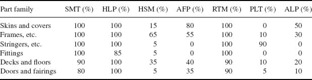
It is immediately obvious from Table 2.2 that no single technology can be used to make an entire airframe in the most cost-effective fashion. There are some portions of certain part families that are more efficiently made by another technology. While the numbers in Table 2.2 are subjective, they reflect what is perceived to be the reality of today and they can be modified according to specific preferences or expected improvements in specific technologies.

Given the applicabilities of Table 2.2, recurring and nonrecurring cost data are obtained or estimated by part family. This is done by calculating or estimating the average cost for a part of medium complexity in the specific part family made by a selected process and determining the standard deviation associated with the distribution of cost around that average as the part complexity ranges from simple to complex parts. This can be done using existing data as is shown in Figure 2.10, for technologies already implemented such as HLP or by extrapolating and approximating limited data from producibility evaluations, vendor information and anticipated improvements for new technologies or technologies with which a particular factory has not had enough experience.

In the case of the data shown in Figure 2.10, data over 34 different skin parts made with hand layup show an average (or mean) cost of 14 h/kg of finished product and a standard deviation around that mean of about 11 h/kg (the horizontal arrows in Figure 2.10 cover approximately two standard deviations). This scatter around the mean cost is mostly due to variations in complexity. A simple skin (flat, constant thickness, no cutouts) can cost as little as 1 h/kg while a complex skin (curved, with ply dropoffs, with cutouts) can cost as high as 30 h/kg. In addition to part complexity, there is a contribution to the standard deviation due to uncertainty. This uncertainty results mainly from two sources [12]: (a) not having enough experience with the process and applying it to types of part to which it has not been applied before; this is referred to as production-readiness; and (b) operator or equipment variability.

Determining the portion of the standard deviation caused by uncertainty is necessary in order to proceed with the selection of the best technology for an application. One way to separate uncertainty from complexity is to use a reliable cost model to predict the cost of parts of different complexity for which actual data are available. The difference between the predictions and the actual data is attributed to uncertainty. By normalizing the prediction by the actual cost for all parts available, a distribution is obtained the standard deviation of which is a measure of the uncertainty associated with the process in question. This standard deviation (or its square, the variance) is an important parameter because it can be associated with the risk. If the predicted cost divided by actual cost data were all in a narrow band around the mean, the risk in using this technology (e.g. HLP) for this part family (e.g. skins) would be very low since the expected cost range would be narrow. Since narrow distributions have low variances, the lower the variance, the lower the risk.

It is more convenient, instead of using absolute cost numbers to use cost savings numbers obtained by comparing each technology of interest with a baseline technology. In what follows, SMT is used as the baseline technology. Positive cost savings numbers denote cost reduction below SMT cost and negative cost savings numbers denote cost increase above SMT costs. Also, generalizing the results from Figure 2.10, it will be assumed that the cost savings for a certain technology applied to a certain part family is normally distributed. Other statistical distributions can be used and, in some cases, will be more accurate. For the purposes of this discussion, the simplicity afforded by assuming a normal distribution is sufficient to show the basic trends and draw the most important conclusions.

By examining data published in the open literature, inferring numbers from trend lines and using experience, the mean cost savings and variances associated with the technologies given in Table 2.2 can be compiled. The results are shown in Table 2.3. Note that these results reflect a specific instant in time and they comprise the best estimate of current costs for a given technology. This means that some learning curve effects are already included in the numbers. For example, HLP and RTM parts have been used fairly widely in industry and factories have come down their respective learning curves. Other technologies such as AFP have not been used as extensively and the numbers quoted are fairly high up in the respective learning curves.

Table 2.3 Typical cost data by technology by part family

For each technology/part family combination in Table 2.3, two numbers are given. The first is the cost savings as a fraction (i.e. 0.17 implies 17% cost reduction compared to SMT) and the second is the variance (square of standard deviation) of the cost savings population. Negative cost savings numbers imply increase in cost over SMT. They are included here because the weight savings may justify the use of the technology even if, on average, the cost is higher. For SMT and some HLP cases, the variance is set to a very low number, 0.0001 to reflect the fact that the cost for these technologies and part families is well understood and there is little uncertainty associated with it. This means the technology has already been in use for that part family for some time. Some of the data in Table 2.3 are highlighted to show some of the implications: (a) HLP skins have 17% lower cost than SMT skin mostly due to co-curing large pieces and eliminating or minimizing assembly; (b) ALP has the lowest cost numbers, but limited applicability (see Table 2.2); (c) the variance in some cases such as ALP decks and floors or AFP doors and fairings is high because for many parts in these families additional nonautomated steps are necessary to complete fabrication. This is typical of sandwich parts containing core where core processing involves manual labour and increases the cost. Manual labour increases the uncertainty due to the operator variability already mentioned.

Given the data in Tables 2.2 and 2.3, one can combine different technologies to make a part family. Doing that over all part families results in a technology mix. This technology mix has an overall mean cost savings and variance associated with it that can be calculated using the data from Tables 2.2 and 2.3 and using the percentages of how much of each part family is made by each technology [12, 13]. This process is shown in Figure 2.11. Obviously, some technology mixes are better than others because they have lower recurring cost and/or lower risk. An optimization scheme can then be set up [13] that aims at determining the technology mix that minimizes the overall recurring cost savings (below the SMT baseline) keeping the associated variance (and thus the risk) below a preselected value. By changing that preselected value from very small (low risk) to very high (high risk) different optimum mixes can be obtained. A typical result of this process is shown in Figure 2.12 for the case of a fuselage and wing of a 20-passenger commuter plane.

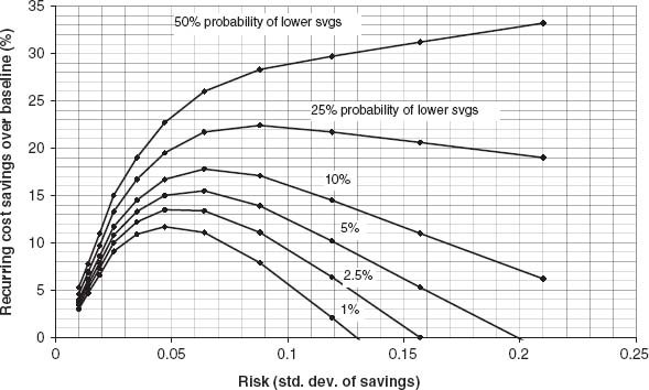
The risk is shown in Figure 2.12 on the x axis as the square root of the variance or standard deviation of the cost savings of the resulting technology mix. For each value of risk, the optimization process results in a technology mix that maximizes cost savings. Assuming that the cost savings of each technology mix is normally distributed, the corresponding probabilities that the cost savings will be lower than a specified value can be determined [13]. These different probabilities trace the different curves shown in Figure 2.12. For example, if the risk is set at 0.05 on the x axis, the resulting optimum mix has 1% probability of not achieving 11.5% savings, 2.5% probability of not achieving 13.5% savings, 5% probability of not achieving 15% savings and so on. Note that all curves, except the 50% probability curve go through a maximum. This maximum can be used for selecting the optimum technology mix to be used. For example, if a specific factory/management team is risk averse it would probably go with the 1% curve which goes through a maximum at a risk value slightly less than 0.05. The team would expect savings of at least 11.5%. A more aggressive team might be comfortable with 25% probability that the cost savings is lower and would use the 25% curve. This has a maximum at a risk value of 0.09 with corresponding savings of 22.5%. However, there is a 25% probability that this level of savings will not be met. That is, if this technology mix were to be implemented a large number of times, it would meet or exceed the 22.5% savings target only 75% of the time. It is up to the management team and factory to decide which risk level and curve they should use. It should be noted that for very high risk values, beyond 0.1, the cost saving curves eventually become negative. For example the 1% curve becomes negative at a risk value of 0.13. This means that the technology mix corresponding to a risk value of 0.13 has so much uncertainty that there is 99% probability that the cost savings will be negative, i.e. the cost will be higher than the SMT baseline.

Once a risk level is selected from Figure 2.12, the corresponding technology mix is known from the optimization process. Examples for low and high risk values are shown in Figures 2.13 and 2.14.

For the low-risk optimum mix of Figure 2.13, there is a 10% probability of not achieving 12.5% cost savings. For the high-risk optimum mix of Figure 2.14 there is a 10% probability of not achieving 7% cost savings. The only reason to go with the high-risk optimum mix is that, at higher probability values (greater than 25%) it exceeds the cost savings of the low-risk optimum mix.

A comparison of Figures 2.14 and 2.13 shows that as the risk increases, the percentage usage of baseline SMT and low-risk low-return HLP and RTM decreases while the usage of higher-risk high-return AFP and ALP increases. ALP usage doubles from 6% to 12% and AFP usage increases by a factor of almost 7, from 3% to 20%. The amount of PLT also increases (in fact doubles), but since PLT is only limited to stringers in this example, the overall impact of using PLT is quite small. It should be noted that there is a portion of the airframe denoted by ‘Misc’. These are miscellaneous parts such as seals or parts for which applicability is unclear and mixing technologies (e.g. pultruded stringers co-bonded on fibre-placed skins) might be a better option, but no data were available for generating predictions.

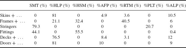
Finally, the breakdown by part family for one of the cases, the low-risk optimum mix of Figure 2.13 is shown in Table 2.4. For example, 21.1% of the frames are made by HLP, 32.4% by HSM, 40.5% by RTM and 6% by ALP. Note that SMT is only used for three quarters of the stringers and almost half the fittings. Note that these percentages are the results of the optimization mentioned earlier and do not exactly determine which parts will be made with what process, only that a certain percentage of parts for each part family is made by a certain process. It is up to the designers and manufacturing personnel to decide how these percentages can be achieved or, if not possible, determine what the best compromise will be. For example, 6% of the frames and bulkheads made by ALP would probably correspond to the pressure bulkheads and any frames with deep webs where automated layup can be used effectively.

Table 2.4 Low-risk technology mix by part family and technology

The above discussion focused on recurring cost as a driver. The optimum technology mixes determined have a certain weight and nonrecurring cost associated with them. If weight or nonrecurring cost were the drivers, different optimum technology mixes would be obtained. Also, the optimized results are frozen in time in the sense that the applicabilities of Table 2.2 and the cost figures of Table 2.3 are assumed constant. Over time, as technologies improve, these data will change and the associated optimum technology mixes will change. Results for the time-dependent problem with different drivers such as nonrecurring cost or optimum return on investment can be found in References 11 and 14.

It should be kept in mind that some of the data used in this section are subjective or based on expectations of what certain technologies will deliver in the future. As such, the results should be viewed as trends that will change with different input data. What is important here is that an approach has been developed that can be used to trade weight, recurring cost and nonrecurring cost and determine the optimum mix of technologies given certain cost data. The interested user of the approach can use his/her own data and degree of comfort in coming up with the optimum mix of technologies for his/her application.

2.4 Summary and Conclusions

An attempt to summarize the above discussion by fabrication process and to collect some of the qualitative considerations that should be taken into account during the design and analysis phases of a program using composite materials is shown in Table 2.5. For reference, sheet metal built-up structure and high-speed-machining (aluminium or titanium) are also included. This table is meant to be a rough set of guidelines and it is expected that different applications and manufacturing experiences can deviate significantly from its conclusions.

Table 2.5 Qualitative cost considerations affecting design/analysis decisions

Process	Application	Comments
Sheet metal	All airframe structure	Assembly intensive, relatively heavy. Moderate tooling costs including fit-out and assembly jigs
High-speed machining	Frames, bulkheads, ribs, beams, decks and floors. In general, parts with one flat surface that can be created via machining	Very low tooling cost. Very low recurring cost. Can generate any desired thickness greater than 0.6 mm. Moderate raw material cost due to the use of special alloys. Extremely high scrap rate (more than 99% of the raw material ends up recycled as machined chips). Limited due to vibrations to part thicknesses greater than 0.6–0.7 mm. Issues with damage tolerance (no built-in crack stoppers) repair methods and low damping; size of billet limits size of part that can be fabricated
Hand layup	All airframe structure	Weight reductions over equivalent metal of at least 15%. Recurring cost competitive with sheet metal when large amount of co-curing is used. Moderate scrap. High raw material cost. High tooling cost. Hard to fabricate 3-D fittings. Reduced out-of-plane strength (important in fittings and parts with out-of-plane loading)
Automated fibre/tow placement	Skins, decks, floors, doors, fairings, bulkheads, large ribs and beams. In general, parts with large surface area	Weight reductions similar to hand layup. Recurring cost can be less than metal baseline if the number of starts and stops for the machine are minimized (few cutouts, plydrops, etc.). Less scrap than hand layup. High tooling cost. For parts made on concave tools, limited by size of robotic head (interference with tool). Fibre steering is promising for additional weight savings but is limited by a maximum radius of curvature the machine can turn without buckling the tows
RTM	All airframe structure	Weight reductions somewhat less than hand layup due to decreased fibre volume for complex parts. Combined with automated preparation of fibre performs it can result in low recurring fabrication cost. Relatively low scrap rate. Very high tooling cost if matched metal tooling is used. Less so for vacuum-assisted RTM (half of the tool is a semi-rigid caul plate) or resin film infusion. To use unidirectional plies, some carrier or tackifier is needed for the fibres, increasing the recurring cost somewhat
Pultrusion	Constant cross-section parts: stiffeners, stringers, small beams	Weight reductions somewhat less than hand layup due to the fact that not all layups are possible (plies with 45° orientation or higher when 0 is aligned with the long axis of the part). Very low recurring cost and relatively low tooling cost compared with other fabrication processes. Reduced strength and stiffness in shear and transverse directions due to inability to generate any desired layup
Filament winding	Concave parts wound on a rotating mandrel: pressure vessels, cylinders, channels (wound and then cut)	Weight reductions somewhat less than hand layup due to difficulty in achieving the required fibre volume and due to inability to achieve certain stacking sequences. Low scrap rate, low raw material cost. Low recurring fabrication cost. Moderate tooling cost. Only convex parts wound on a mandrel where the tension in the fibres can be maintained during fabrication. Cannot wind angles shallower than geodetic lines (angles less than 15° not possible for long slender parts with 0 aligned with the long axis of the part). Reduced strength and stiffness
Press moulding	Fittings, clips, shear ties, small beams, ribs, intercostals	Weight reductions in the range 10–20% over aluminium baseline (weight savings potential limited due to the use of discontinuous fibres). Very low recurring cost with very short production cycle (minutes to a couple of hours). Low material scrap. Limited by the size of the press. Very high tooling cost for the press mould. Reduced strength due to the use of long discontinuous fibres, but good out-of-plane strength due to ‘interlocking’ of fibres

As shown in the previous section, there is no single process that can be applied to all types of parts and result in the lowest recurring and/or nonrecurring costs. A combination of processes is necessary. In many cases, combining two or more processes in fabricating a single part, thus creating a hybrid process (e.g. automated fibre-placed skins with staged pultruded stiffeners, all co-cured in one cure cycle) appears to be the most efficient approach. In general, co-curing as large parts as possible and combining with as much automation as possible seems to have the most promise for parts of low cost, high quality and consistency. Of course, the degree to which this can be done depends on how much risk is considered acceptable in a specific application and to what extent the investment required to implement more than one fabrication processes is justified by the size of the production run. These combinations of processes and process improvements have already started to pay off and, for certain applications [15], the cost of composite airframe is comparable if not lower than that of equivalent metal structure.

Exercises

2.1 Hand layup, resin transfer moulding and press moulding are considered as the candidate processes for the following part:

2.2 Hand layup, automated fibre placement and filament winding are proposed as candidate processes for the following part:

2.3 A certain composites technology is considered for implementation in a factory for the first time to make composite parts for airplanes. This technology requires new equipment that costs $1.5 million. In addition, experts estimate that the nonrecurring cost for each new part the factory makes with the new technology (design, analysis, … all the way to certification) is, on the average, $20, 000/kg of structure replaced. The technology has 25% applicability (by weight) over a structure that weighs 42, 000 kg. The experts also expect that the new technology will save 15% of the weight of the structure it replaces (which is the reason for considering the switch to the new technology; it makes it more attractive to the customer) and it will start two times more expensive than the structure it replaces which, currently, costs 3.5 h/kg. It will also go down a 90.5% learning curve. How many aircraft must they sell to get their investment back if the hourly rate (including overhead) for the factory is 150$/h in one plant and 95$/h in another? (Give two answers; one for implementing the technology in one plant and one in the other). Make a plot showing the total $ “savings” as a function of number of aircraft sold for the two different factory hourly rates. Assume that the baseline technology is already far enough down its own learning curve so its cost will not change over time. Also assume that for every kilogram saved, the customer is willing to pay an extra $250. (Note that in this simplification of the problem, the time element, inflation, cost escalation, return on investment calculations, etc. are neglected.)

References

[1] Gutowski, T.G., Hoult, D., Dillon, G., Mutter, S., Kim, E., Tse, M., and Neoh, E.T., Development of a Theoretical Cost Model for Advanced Composite Fabrication, Proc. 4th NASA/DoD Advanced Composites Technology Conf., Salt Lake City, UT, 1993.

[2] Gutowski, T.G., Neoh, E.T., and Dillon, G., Scaling Laws for Advanced Composites Fabrication Cost, Proc. 5th NASA/DoD Advanced Composites Technology Conf., Seattle, WA, 1994, pp. 205–233.

[3] Apostolopoulos, P., and Kassapoglou, C., Cost Minimization of Composite Laminated Structures – Optimum Part Size as a Function of Learning Curve Effects and Assembly, Journal of Composite Materials, 36(4), 501–518 (2002).

[4] Tatting, B., and Gürdal, Z., Design and Manufacture of Elastically Tailored Tow-Placed Plates, NASA CR 2002 211919, August 2002.

[5] Jegley, D., Tatting, B., and Gürdal, Z., Optimization of Elastically Tailored Tow-Placed Plates with Holes, 44th AIAA/ASME/ASCE/AHS Structures, Structural Dynamics and Materials Conf., Norfolk VA, 2003, also paper AIAA-2003-1420.

[6] 1st NASA Advanced Composites Technology Conf., NASA CP 3104, Seattle WA, 1990.

[7] 2nd NASA Advanced Composites Technology Conf., NASA CP 3154, Lake Tahoe, NV, 1991.

[8] Abbott, R., Design and Certification of the All-Composite Airframe. Society of Automotive Engineers Technical Paper Series – Paper No 892210; 1989.

[9] Whitehead, R.S., Kan, H.P., Cordero, R. and Saether, E.S., Certification Testing Methodology for Composite Structures: Volume I – Data Analysis. Naval Air Development Center Report 87042-60(DOT/FAA/CT-86-39); 1986.

[10] Whitehead, R.S., Kan, H.P., Cordero, R. and Saether, E.S., Certification Testing Methodology for Composite Structures: Volume II – Methodology Development. Naval Air Development Center Report 87042-60 (DOT/FAA/ CT-86-39); 1986.

[11] Kassapoglou, C., Determination of the Optimum Implementation Plan for Manufacturing Technologies – The case of a Helicopter Fuselage, Journal of Manufacturing Systems, 19, 121–133 (2000).

[12] Kassapoglou, C., Selection of Manufacturing Technologies for Fuselage Structures for Minimum Cost and Low Risk: Part A – Problem Formulation, Journal of Composites Technology and Research, 21, 183–188 (1999).

[13] Kassapoglou, C., Selection of Manufacturing Technologies for Fuselage Structures for Minimum Cost and Low risk: Part B – Solution and Results, Journal of Composites Technology and Research, 21, 189–196 (1999).

[14] Sarkar, P. and Kassapoglou, C., An ROI-Based Strategy for Implementation of Existing and Emerging Technologies, Spring Research Conf. on Statistics in Industry and Technology, Minneapolis-St Paul, MN, June 1999. Also IEEE Transactions on Engineering Management, 48, 414–427 (1999).

[15] McGettrick, M., and Abbott, R., To MRB or not to be: Intrinsic Manufacturing Variabilities and Effects on Load Carrying Capacity, Proc. 10th DoD/NASA/FAA Conf. on Fibrous Composites in Structural Design, Hilton Head, SC, 1993, pp. 5–39.