
Chapter 8
Dynamic Range Control
U. Zölzer and E. Gerat
The dynamic range of a signal is defined as the logarithmic ratio of maximum to minimum signal amplitude and is given in decibels. The dynamic range of an audio signal lies between 40 and 120 dB. Dynamic range control of audio signals is used in many applications to match the dynamic behavior of the audio signal to different requirements. While recording, dynamic range control protects the AD converter from overload or it is used in the signal path to optimally use the full amplitude range of a recording system. For suppressing low‐level noise, so‐called noise gates are used so that the audio signal is passed through only from a certain level onward. While reproducing music and speech in a car, a shopping center, restaurant, or inside a disco, the dynamics have to match the special noise characteristic of the environment. Therefore the signal level is measured from the audio signal and a control signal is derived which then changes the signal level to control the loudness of the audio signal. This loudness control is adaptive to the input level. The combination of level measurement and adaptive signal level adjustment is called dynamic range control.
8.1 Basics
Figure 8.1 shows a block diagram of a system for dynamic range control. After measuring the input level ![]() , the output level
, the output level ![]() is affected by multiplying the delayed input signal
is affected by multiplying the delayed input signal ![]() by a factor
by a factor ![]() according to
according to
The delay of the signal ![]() compared with the control signal
compared with the control signal ![]() allows predictive control of the output signal level. This multiplicative weighting is carried out with corresponding attack and release time. Multiplication leads, in terms of a logarithmic level representation of the corresponding signals, to the addition of the weighting level
allows predictive control of the output signal level. This multiplicative weighting is carried out with corresponding attack and release time. Multiplication leads, in terms of a logarithmic level representation of the corresponding signals, to the addition of the weighting level ![]() to the input level
to the input level ![]() giving the output level
giving the output level
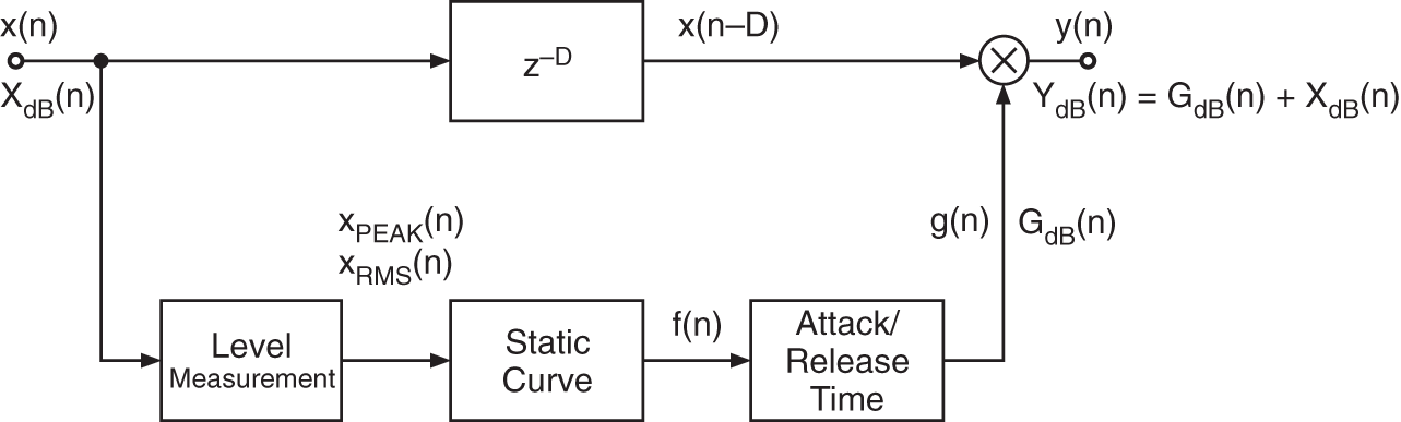
Figure 8.1 System for dynamic range control.
8.2 Static Curve
The relationship between input level and weighting level is defined by a static level curve ![]() . An example of such a static curve is given in Fig. 8.2. Here, the output level and the weighting level are given as functions of the input level.
. An example of such a static curve is given in Fig. 8.2. Here, the output level and the weighting level are given as functions of the input level.
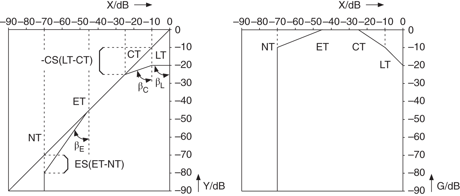
Figure 8.2 Static curve with the parameters: LT = limiter threshold; CT = compressor threshold; ET = expander threshold; and NT = noise gate threshold.
With the help of a limiter, the output level is limited when the input level exceeds the limiter threshold (LT). All input levels above this threshold lead to a constant output level. The compressor maps a change of input level on a certain smaller change of output level. In contrast to a limiter, the compressor increases the loudness of the audio signal. The expander increases changes in the input level to larger changes in the output level. With this, an increase of the dynamics for low levels is achieved. The noise gate is used to suppress low‐level signals, for noise reduction, and is also used for sound effects like truncating the decay of room reverberation. Every threshold used in particular parts of the static curve is defined as the lower limit for the limiter and compressor and upper limit for the expander and noise gate.
In the logarithmic representation of the static curve, the compression factor R (ratio) is defined by the ratio of the input level change ![]() to the output level change
to the output level change ![]() , as given by
, as given by


Figure 8.3 Compressor curve (compressor ratio CR/compressor slope CS).
With the help of Fig. 8.3, the straight line equation ![]() and the compression factor
and the compression factor
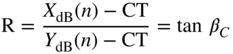
are obtained, where the angle ![]() is defined as shown in Fig. 8.2. The relationship between the ratio R and the slope S can also be derived from Fig. 8.3 and is expressed as
is defined as shown in Fig. 8.2. The relationship between the ratio R and the slope S can also be derived from Fig. 8.3 and is expressed as
Typical compression factors are
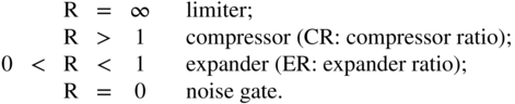
The transition from logarithmic to linear representation leads, from Eq. (8.4), to
where ![]() and
and ![]() are the linear levels and
are the linear levels and ![]() denotes the linear compressor threshold. Rewriting Eq. (8.8) gives the linear output level
denotes the linear compressor threshold. Rewriting Eq. (8.8) gives the linear output level
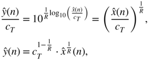
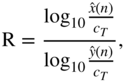
as a function of input level. The control factor ![]() can be calculated by the quotient
can be calculated by the quotient

With the help of tables and interpolation methods, it is possible to determine the control factor without taking logarithms and antilogarithms. The implementation described as follows, however, makes use of the logarithm of the input level and calculates the control level ![]() with the help of the straight line equation. The antilogarithm leads to the value
with the help of the straight line equation. The antilogarithm leads to the value ![]() which gives the control factor
which gives the control factor ![]() with corresponding attack and release times (see Fig. 8.1).
with corresponding attack and release times (see Fig. 8.1).
To further smoothen the transition between the compressed (or expanded) and uncompressed portions of the static curve at the threshold level, the width ![]() of the knee (angle at the threshold) can be adjusted. A width set to zero will give a hard knee while a larger width will set what is called a soft knee. It consists of a range centered on the threshold level with a variable width, as shown in Fig. 8.4. This allows a more transparent dynamic range control operation. The knee portion of the static curve is replaced by a piecewise continuous function
of the knee (angle at the threshold) can be adjusted. A width set to zero will give a hard knee while a larger width will set what is called a soft knee. It consists of a range centered on the threshold level with a variable width, as shown in Fig. 8.4. This allows a more transparent dynamic range control operation. The knee portion of the static curve is replaced by a piecewise continuous function
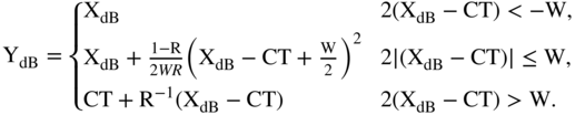
The make‐up gain is an additional gain used to compensate the level loss produced by the compression operation. It allows the generation of a sound perceived to be louder without the distortions induced by the clipping of the audio signal.
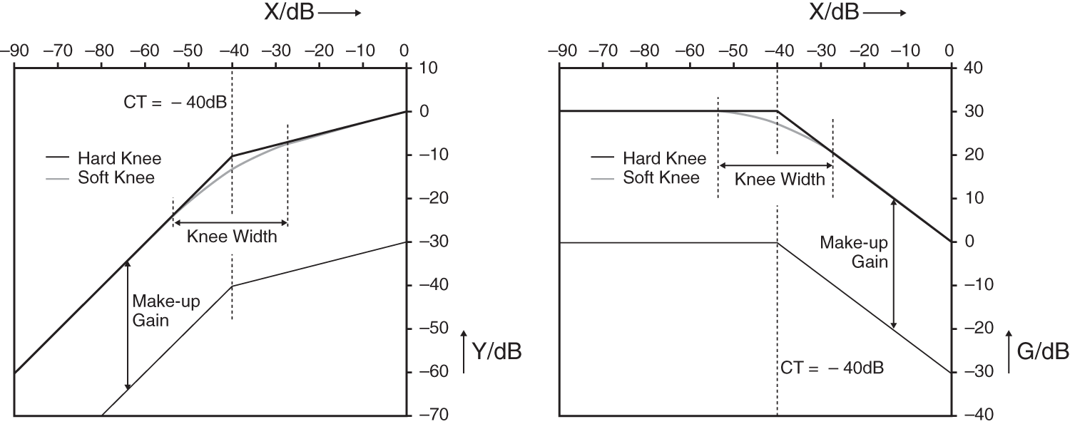
Figure 8.4 Static curve and gain mapping curve of a compressor with soft and hard knees and make‐up gain.
8.3 Dynamic Behavior
In addition to the static curve of dynamic range control, the dynamic behavior in terms of attack and release times plays a significant role in sound quality. The rapidity of dynamic range control depends also on the measurement of PEAK and RMS values [McN84, Sti86].
8.3.1 Level Measurement
Level measurements [McN84] can be performed with the systems shown in Figs. 8.5 and 8.9. For PEAK measurement, the absolute value of the input is compared with the peak value ![]() . If the absolute value is greater than the peak value, the difference is weighted with the coefficient AT (attack time) and added to
. If the absolute value is greater than the peak value, the difference is weighted with the coefficient AT (attack time) and added to ![]() . For this attack case
. For this attack case ![]() , we get the difference equation (see Fig. 8.5)
, we get the difference equation (see Fig. 8.5)
with the transfer function
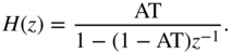
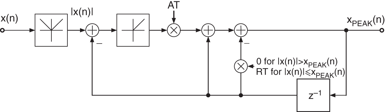
Figure 8.5 PEAK measurement.
If the absolute value of the input is smaller than the peak value ![]() (the release case), the new peak value is given by
(the release case), the new peak value is given by
with the release time coefficient RT. The difference signal of the input will be muted by the nonlinearity such that the difference equation for the peak value is given according to Eq. (8.14). For the release case, the transfer function
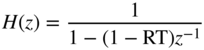
is valid. For the attack case, the transfer function (8.13) with coefficient AT is used, and for the release case, the transfer function (8.15) with the coefficient RT is used. The coefficients (see Section 8.3.3) are given by
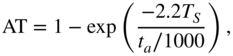
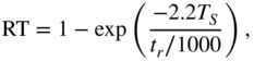
where the attack time ![]() and the release time
and the release time ![]() are given in msec (
are given in msec (![]() sampling interval). With this switching between filter structures, one achieves fast attack responses for increasing input signal amplitudes and slow decay responses for decreasing input signal amplitudes.
sampling interval). With this switching between filter structures, one achieves fast attack responses for increasing input signal amplitudes and slow decay responses for decreasing input signal amplitudes.
A first variation for peak detection is the branched peak detector that has two different branches of operation, as shown in Fig. 8.6. For the attack case AC when ![]() and the release case RC when
and the release case RC when ![]() , the operations are given by
, the operations are given by
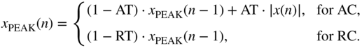
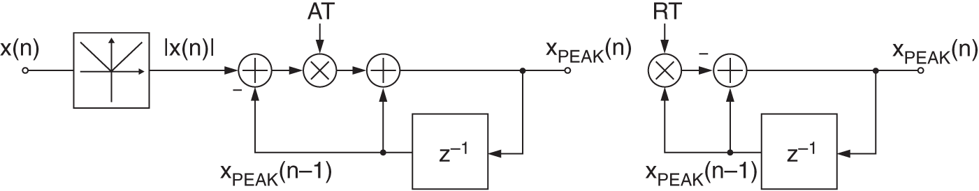
Figure 8.6 Block diagrams of the attack and release parts of the branched peak level detector.
One further variation of the peak detector is the so‐called decoupled peak level detector, which is presented in Fig. 8.7. It computes an auxiliary signal ![]() based on the release time and then feeds this signal to an attack filter, as given by
based on the release time and then feeds this signal to an attack filter, as given by
This detector adds a small onset to the release time, as shown in Fig. 8.8. This leads to the release time approximately equal to ![]() and is therefore always bigger than the attack time. This can be useful to avoid artifacts arising from release times that are too short [Gia12].
and is therefore always bigger than the attack time. This can be useful to avoid artifacts arising from release times that are too short [Gia12].
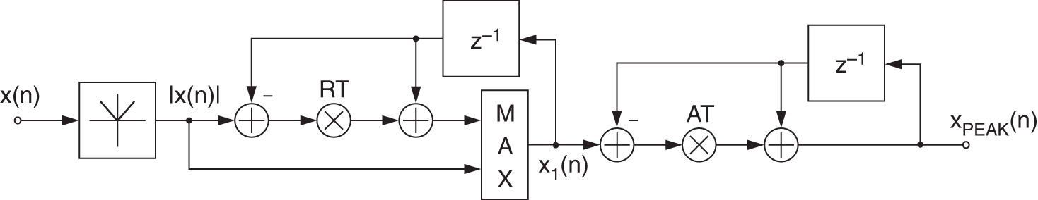
Figure 8.7 Block diagram of the decoupled peak level detector.
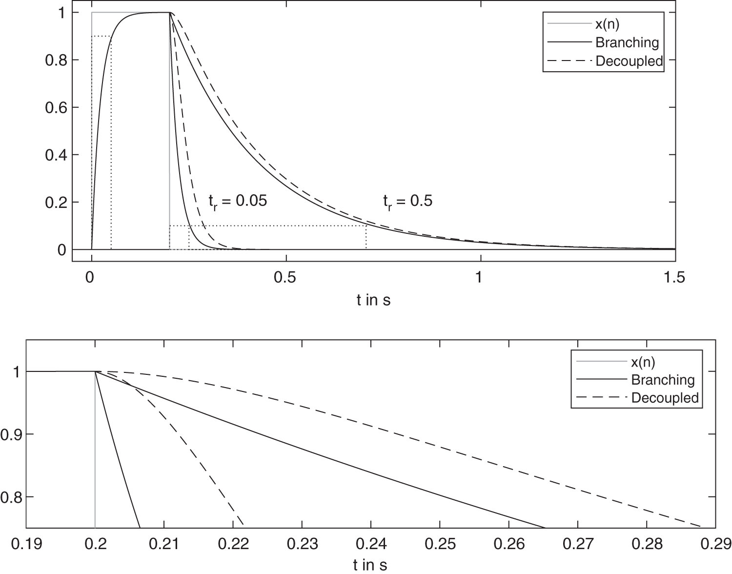
Figure 8.8 Attack and release behavior of branching and decoupled peak level detectors.
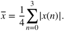
The computation of the RMS value
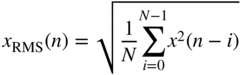
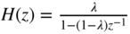
over ![]() input samples can be achieved by a recursive formulation. The RMS measurement shown in Fig. 8.9 uses the square of the input and performs averaging with a first‐order lowpass filter. The averaging coefficient
input samples can be achieved by a recursive formulation. The RMS measurement shown in Fig. 8.9 uses the square of the input and performs averaging with a first‐order lowpass filter. The averaging coefficient
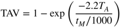
is determined according to the time constant calculation discussed in Section 8.3.3, where ![]() is the averaging time in msec. The difference equation is given by
is the averaging time in msec. The difference equation is given by
with the transfer function
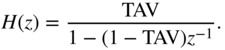
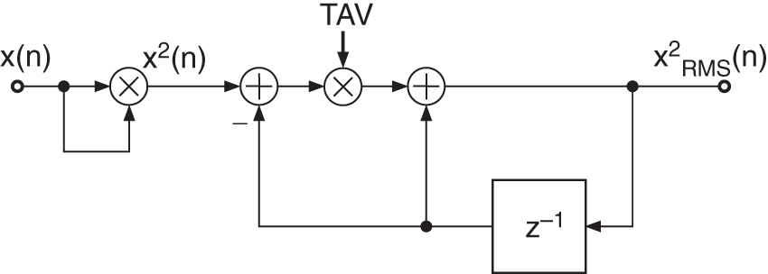
Figure 8.9 RMS measurement (TAV = averaging coefficient).
8.3.2 Gain Factor Smoothing
Attack and release times can be implemented by the system shown in Fig. 8.10 [McN84]. The attack coefficient AT or release coefficient RT is obtained by comparing the input control factor with the previous one. A small hysteresis curve determines whether the control factor is in the attack or release status and hence gives the coefficient AT or RT. The system also serves to smooth the control signal. The difference equation is given by
with ![]() or
or ![]() and the corresponding transfer function leads to
and the corresponding transfer function leads to
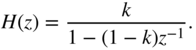
Figure 8.10 Implementing attack and release times or gain factor smoothing.
8.3.3 Time Constants
If the step response of a continuous‐time system is
then sampling (step‐invariant transform) the step response gives the discrete‐time step response
The Z‐transform leads to
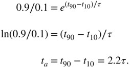
With the definition of attack time ![]() , we derive
, we derive
The relationship between attack time ![]() and the time constant
and the time constant ![]() of the step response is obtained as follows:
of the step response is obtained as follows:
Hence, the pole is calculated as
A system for implementing the given step response is obtained by the relationship between the Z‐transform of the impulse response and the Z‐transform of the step response:
The transfer function can now be written as
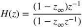
with the pole ![]() adjusting the attack, release, or averaging time. For the coefficients of the corresponding time constant filters, the attack case is given by Eq. (8.16), the release case by Eq. (8.17), and the averaging case by Eq. (8.22). Figure 8.11 shows an example where the dotted lines mark the
adjusting the attack, release, or averaging time. For the coefficients of the corresponding time constant filters, the attack case is given by Eq. (8.16), the release case by Eq. (8.17), and the averaging case by Eq. (8.22). Figure 8.11 shows an example where the dotted lines mark the ![]() and
and ![]() times.
times.
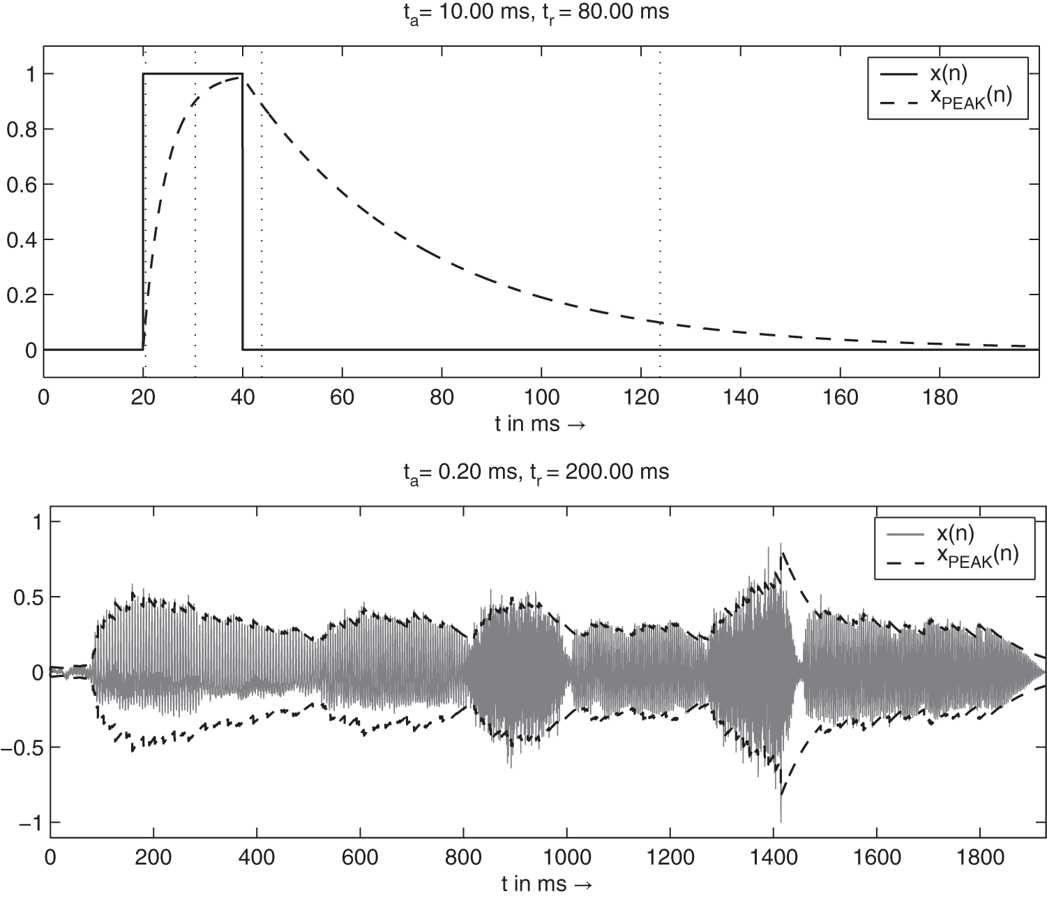
Figure 8.11 Attack and release behavior for time constant filters.
8.4 Implementation
The programming of a system for dynamic range control is described in the following sections.
8.4.1 Limiter
The block diagram of a limiter is presented in Fig. 8.12. The signal ![]() is determined from the input with variable attack and release times. The logarithm to the base 2 of this peak signal is taken and compared with the limiter threshold. If the signal is above the threshold, the difference is multiplied by the negative slope of the limiter LS. After this, the antilogarithm of the result is taken. The obtained control factor
is determined from the input with variable attack and release times. The logarithm to the base 2 of this peak signal is taken and compared with the limiter threshold. If the signal is above the threshold, the difference is multiplied by the negative slope of the limiter LS. After this, the antilogarithm of the result is taken. The obtained control factor ![]() is then smoothed with a first‐order lowpass filter (SMOOTH). If the signal
is then smoothed with a first‐order lowpass filter (SMOOTH). If the signal ![]() lies below the limiter threshold, the signal
lies below the limiter threshold, the signal ![]() is set to
is set to ![]() . The delayed input
. The delayed input ![]() is multiplied by the smoothed control factor
is multiplied by the smoothed control factor ![]() to give the output
to give the output ![]() .
.
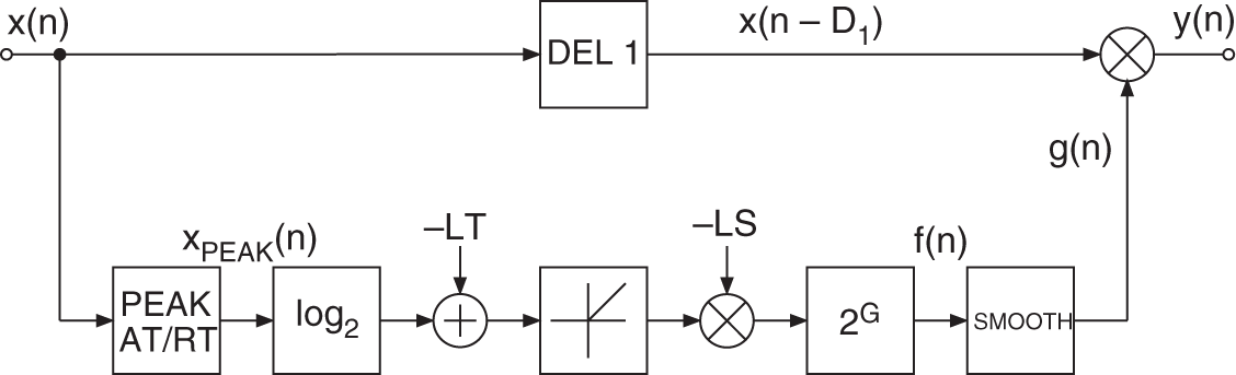
Figure 8.12 Limiter.
8.4.2 Compressor
Feedback implementation
A DRC system can be implemented in a feedback form, as shown in Fig. 8.13, where level sensing is performed on the output signal ![]() . A delay has to be introduced in the feedback side‐chain path. The gain is then applied to the input signal
. A delay has to be introduced in the feedback side‐chain path. The gain is then applied to the input signal ![]() .
.
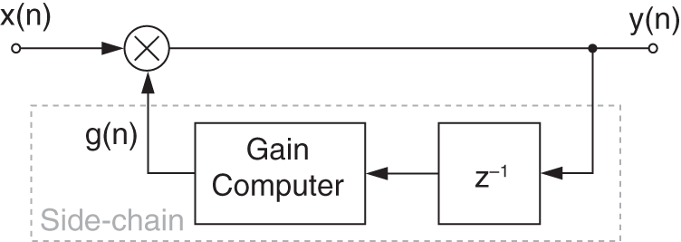
Figure 8.13 Feedback DRC System.
Ducking
Ducking consists of using a second signal ![]() as input to the side‐chain of the DRC system, as shown in Fig. 8.14. This has various applications, for example, in the case of background music playing and an announcement has to be made. The level of the music can be automatically reduced by sensing the level of the speaker and thus applying a negative gain to the music (compression). This effect is also widely used in modern music production to give a stronger feeling of energy to the kick drum. In this case, the kick drum is used as a side‐chain signal to periodically attenuate the rest of the instruments.
as input to the side‐chain of the DRC system, as shown in Fig. 8.14. This has various applications, for example, in the case of background music playing and an announcement has to be made. The level of the music can be automatically reduced by sensing the level of the speaker and thus applying a negative gain to the music (compression). This effect is also widely used in modern music production to give a stronger feeling of energy to the kick drum. In this case, the kick drum is used as a side‐chain signal to periodically attenuate the rest of the instruments.
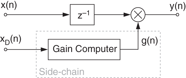
Figure 8.14 Ducking DRC system.
Lookahead
The lookahead consists of introducing a delay in the direct path to sense the level prior to applying it, as shown in Fig. 8.15. It is useful when applied on transients or fast changing signals, because it predicts the variations and reduces (or avoids) the time needed to react to changes in the signal dynamic. When realized offline, the delay introduced can be compensated, but in real‐time, the delay is equal to the lookahead time. Given a lookahead time ![]() in ms, the number of samples is given by
in ms, the number of samples is given by ![]() .
.
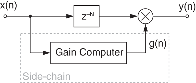
Figure 8.15 DRC system with a lookahead of  samples.
8.4.3 Compressor, Expander, Noise Gate
The block diagram of a compressor/expander/noise gate is shown in Fig. 8.16. The basic structure is similar to the limiter. In contrast to the limiter, the logarithm of the signal ![]() is taken and multiplied by 0.5. The obtained value is compared with three thresholds to determine the operating range of the static curve. If one of the three thresholds is crossed, the resulting difference is multiplied by the corresponding slope (CS, ES, NS) and the antilogarithm of the result is taken. A following first‐order lowpass filter provides the attack and release times.
is taken and multiplied by 0.5. The obtained value is compared with three thresholds to determine the operating range of the static curve. If one of the three thresholds is crossed, the resulting difference is multiplied by the corresponding slope (CS, ES, NS) and the antilogarithm of the result is taken. A following first‐order lowpass filter provides the attack and release times.
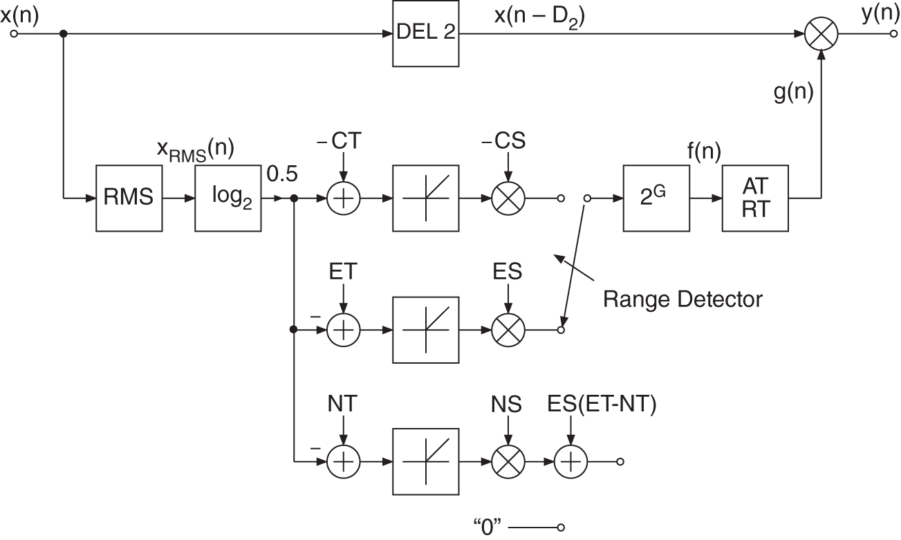
Figure 8.16 Compressor/expander/noise gate.
8.4.4 Combination System
A combination of a limiter that uses PEAK measurement and a compressor/expander/noise gate that is based on RMS measurement, is presented in Fig. 8.17. The PEAK and RMS values are measured simultaneously. If the linear threshold of the limiter is crossed, the logarithm of the peak signal ![]() is taken and the upper path of the limiter is used to calculate the characteristic curve. If the limiter threshold is not crossed, the logarithm of the RMS value is taken and one of the three lower paths is used. The additive terms in the limiter and noise gate paths result from the static curve. After going through the range detector, the antilogarithm is taken. The sequence
is taken and the upper path of the limiter is used to calculate the characteristic curve. If the limiter threshold is not crossed, the logarithm of the RMS value is taken and one of the three lower paths is used. The additive terms in the limiter and noise gate paths result from the static curve. After going through the range detector, the antilogarithm is taken. The sequence ![]() is smoothed with a SMOOTH filter in the limiter case, or weighted with corresponding attack and release times of the relevant operating range (compressor, expander, or noise gate). By limiting the maximum level, the dynamic range is reduced. As a consequence, the overall static curve can be shifted up by a gain factor. Figure 8.18 demonstrates this with a gain factor equal to 10 dB. This static parameter value is directly included in the control factor
is smoothed with a SMOOTH filter in the limiter case, or weighted with corresponding attack and release times of the relevant operating range (compressor, expander, or noise gate). By limiting the maximum level, the dynamic range is reduced. As a consequence, the overall static curve can be shifted up by a gain factor. Figure 8.18 demonstrates this with a gain factor equal to 10 dB. This static parameter value is directly included in the control factor ![]() .
.
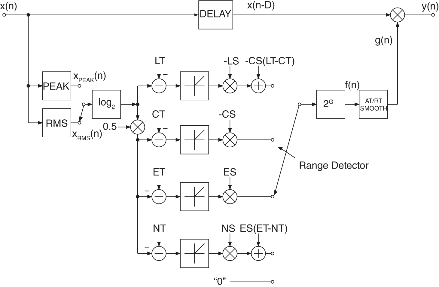
Figure 8.17 Limiter/compressor/expander/noise gate.
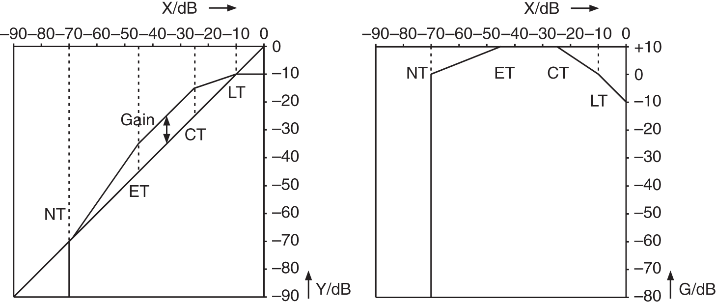
Figure 8.18 Shifting the static curve by a gain factor.
As an example, Fig. 8.19 illustrates the input ![]() , the output
, the output ![]() , and the control factor
, and the control factor ![]() of a compressor/expander system. It is observed that signals with high amplitude are compressed and those with low amplitude are expanded. An additional gain of 12 dB shows the maximum value of 4 for the control factor
of a compressor/expander system. It is observed that signals with high amplitude are compressed and those with low amplitude are expanded. An additional gain of 12 dB shows the maximum value of 4 for the control factor ![]() . The compressor/expander system operates in the linear region of the static curve if the control factor is equal to 4. If the control factor is between 1 and 4, the system operates as a compressor. For control factors lower than 1, the system works as an expander (
. The compressor/expander system operates in the linear region of the static curve if the control factor is equal to 4. If the control factor is between 1 and 4, the system operates as a compressor. For control factors lower than 1, the system works as an expander (![]() and
and ![]() ). The compressor is responsible for increasing the loudness of the signal whereas the expander increases the dynamic range for signals of small amplitude.
). The compressor is responsible for increasing the loudness of the signal whereas the expander increases the dynamic range for signals of small amplitude.
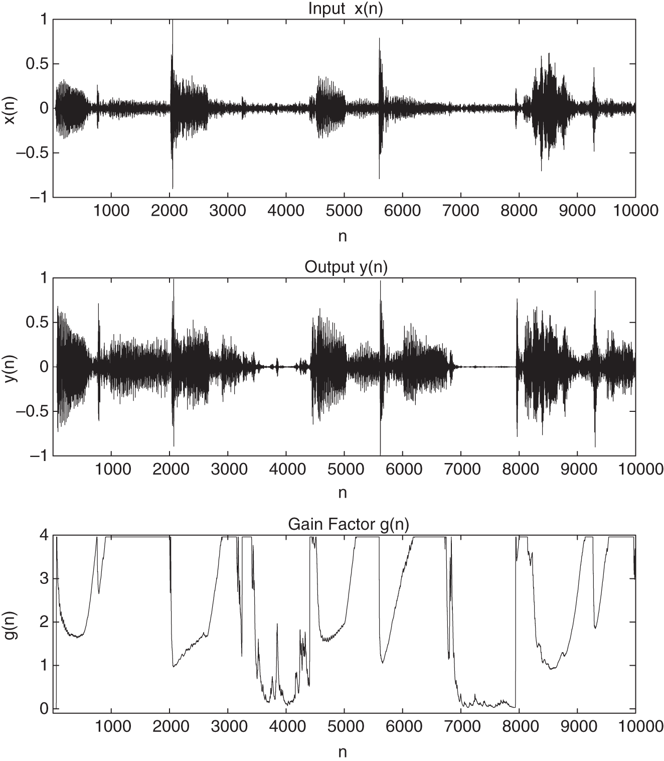
Figure 8.19 Signals  ,
,  , and
, and  for dynamic range control.
8.5 Realization Aspects
8.5.1 Sampling Rate Reduction
To reduce the computational complexity, downsampling can be carried out after calculating the PEAK/RMS value (see Fig. 8.20). As the signals ![]() and
and ![]() are already band limited, they can be directly downsampled by taking every second or fourth value of the sequence. This downsampled signal is then processed by taking its logarithm, calculating the static curve, taking the antilogarithm, and filtering with corresponding attack and release time with reduced sampling rate. A following upsampling by a factor of 4 is achieved by repeating the output value four times. This procedure is equivalent to upsampling by a factor 4 followed by a sample‐and‐hold transfer function.
are already band limited, they can be directly downsampled by taking every second or fourth value of the sequence. This downsampled signal is then processed by taking its logarithm, calculating the static curve, taking the antilogarithm, and filtering with corresponding attack and release time with reduced sampling rate. A following upsampling by a factor of 4 is achieved by repeating the output value four times. This procedure is equivalent to upsampling by a factor 4 followed by a sample‐and‐hold transfer function.
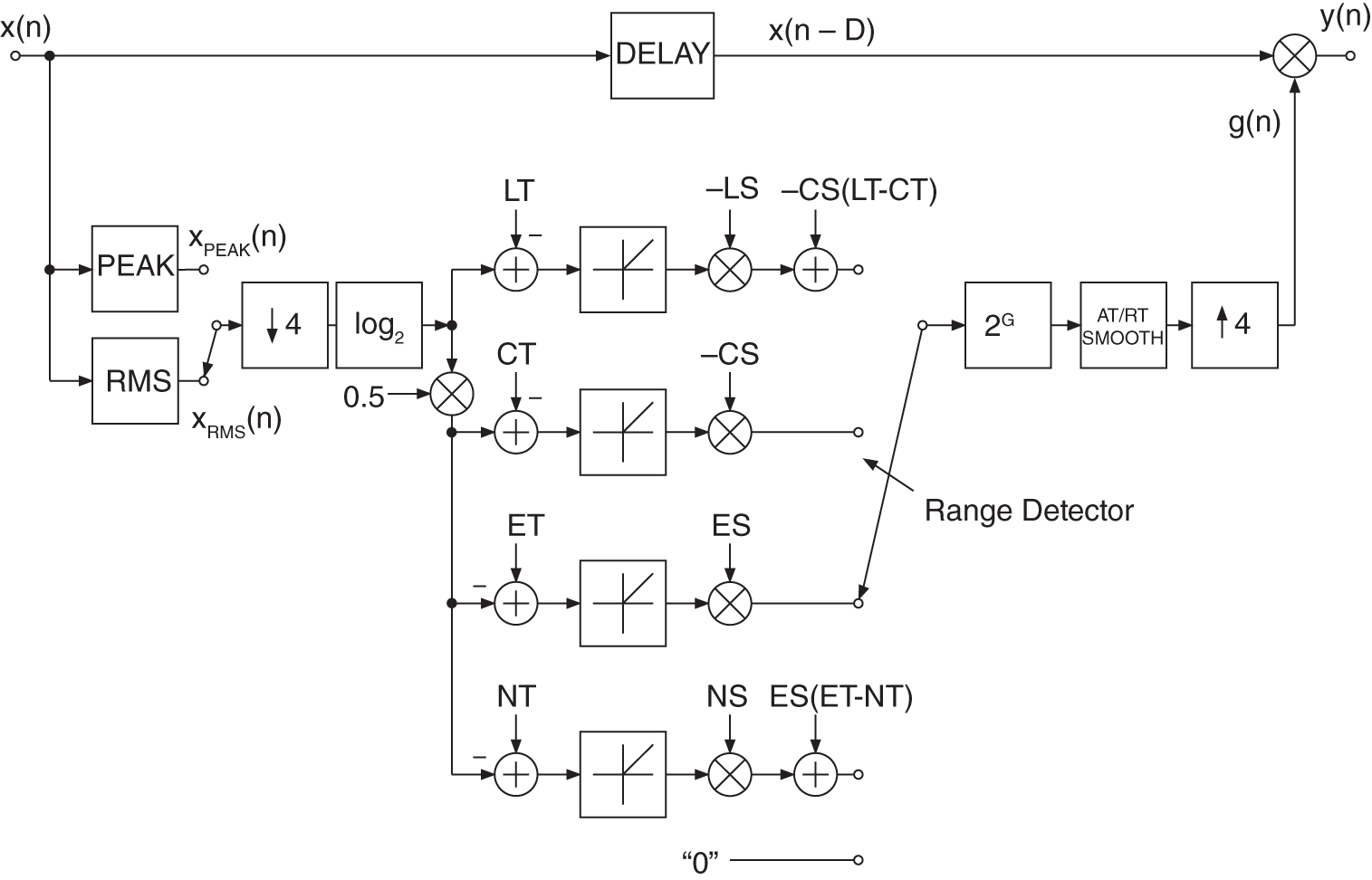
Figure 8.20 Dynamic system with sampling rate reduction.
The nesting and spreading of partial program modules over four sampling periods is shown in Fig. 8.21. The modules PEAK/RMS (i.e. PEAK/RMS calculation) and MULT (delay of input and multiplication with ![]() ) are performed every input sampling period. The number of processor cycles for PEAK/RMS and MULT are denoted by Z1 and Z3, respectively. The modules LD(x), CURVE,
) are performed every input sampling period. The number of processor cycles for PEAK/RMS and MULT are denoted by Z1 and Z3, respectively. The modules LD(x), CURVE, ![]() , and SMO have a maximum number of processor cycles of Z2 and are processed consecutively in the given order. This procedure is repeated every four sampling periods. The total number of processor cycles per sampling period for the complete dynamics algorithm results from the sum of all three modules.
, and SMO have a maximum number of processor cycles of Z2 and are processed consecutively in the given order. This procedure is repeated every four sampling periods. The total number of processor cycles per sampling period for the complete dynamics algorithm results from the sum of all three modules.
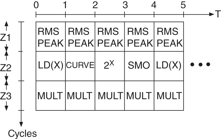
Figure 8.21 Nesting technique.
8.5.2 Curve Approximation
In addition to taking the logarithm and antilogarithm, other simple operations like comparisons and addition/multiplication occur in calculating the static curve. The logarithm of the PEAK/RMS value is taken as follows:
First, the mantissa is normalized and the exponent is determined. The function ![]() is then calculated by a series expansion. The exponent is simply added to the result.
is then calculated by a series expansion. The exponent is simply added to the result.
The logarithmic weighting factor ![]() and the antilogarithm
and the antilogarithm ![]() are given by
are given by
Here, ![]() is a natural number and
is a natural number and ![]() is a fractional number. The antilogarithm
is a fractional number. The antilogarithm ![]() is calculated by expanding the function
is calculated by expanding the function ![]() in a series and multiplication by
in a series and multiplication by ![]() . A reduction of computational complexity can be achieved by directly using tables for log and antilog.
. A reduction of computational complexity can be achieved by directly using tables for log and antilog.
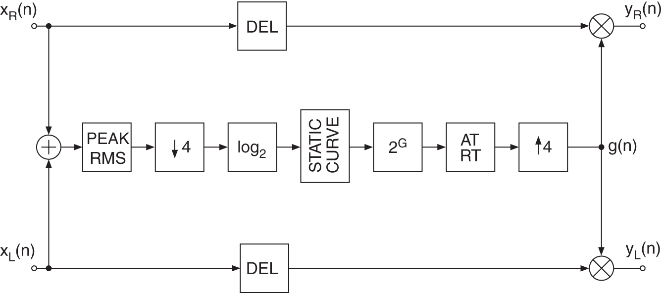
Figure 8.22 Stereo dynamic system.
8.5.3 Stereo Processing
For stereo processing, a common control factor ![]() is needed. If different control factors are used for both channels, limiting or compressing one of the two stereo signals causes a displacement of the stereo balance. Figure 8.22 shows a stereo dynamic system in which the sum of the two signals is used to calculate a common control factor
is needed. If different control factors are used for both channels, limiting or compressing one of the two stereo signals causes a displacement of the stereo balance. Figure 8.22 shows a stereo dynamic system in which the sum of the two signals is used to calculate a common control factor ![]() . The following processing steps of measuring the PEAK/RMS value, downsampling, taking logarithm, calculating static curve, taking antilogarithm attack and release time, and upsampling with a sample‐and‐hold function remain the same. The delay (DEL) in the direct path must be the same for both channels.
. The following processing steps of measuring the PEAK/RMS value, downsampling, taking logarithm, calculating static curve, taking antilogarithm attack and release time, and upsampling with a sample‐and‐hold function remain the same. The delay (DEL) in the direct path must be the same for both channels.
8.6 Multiband DRC
A multiband DRC system consists of several DRC devices applied on different portions of the frequency range. The signal is split into bands (usually 3 to 5) with a complementary filter bank and each band is treated separately with it own DRC device (usually a compressor), as shown in Fig. 8.23. Multiband compressors are useful when only a specific frequency region of the signal has to be treated. Especially at the mastering stage where the mix is already done, each instrument can not be treated on its own anymore. It also prevents common DRC artifacts that occur over a wider frequency range. The level is measured on each band and is used for the gain computation of the corresponding DRC device [Dut11]. A problem of multiband compressors is that the signal is split into bands even when the device is not active. This can cause filtering problems, such as phase cancellation or shifting, making the effect not fully transparent even when deactivated. Also important to notice is that such systems are relatively expensive to compute and can lead to CPU overload when heavily used on systems that are too weak.
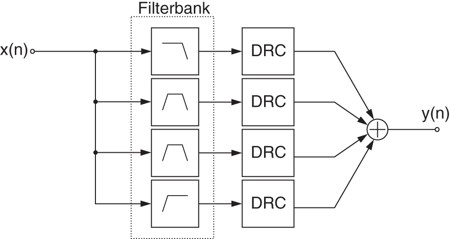
Figure 8.23 Multiband DRC system.
8.7 Dynamic Equalizers
Dynamic equalizers are very similar to multiband DRC systems, but are in their own way more transparent. The filters for a dynamic equalizer are placed in series like a regular equalizer, but the sensing can be performed in parallel, as shown in Fig. 8.24. The levels of several band‐limited signals are sensed and are used to control the gain of a peak (or shelving) filter. The control can be positive and work as an expander (the gain of the filter is proportional to the gain which exceeds the threshold), or can also be negative and work as a compressor (the filter gain is inverse proportional to the gain exceeding the threshold) [Wis09, Väl16]. A corresponding frequency response at a specific time instant ![]() is shown in Fig. 8.25.
is shown in Fig. 8.25.
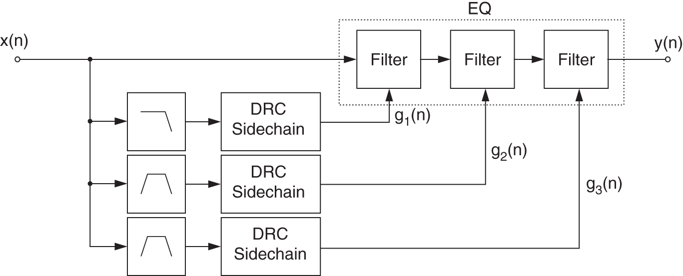
Figure 8.24 Dynamic EQ system.
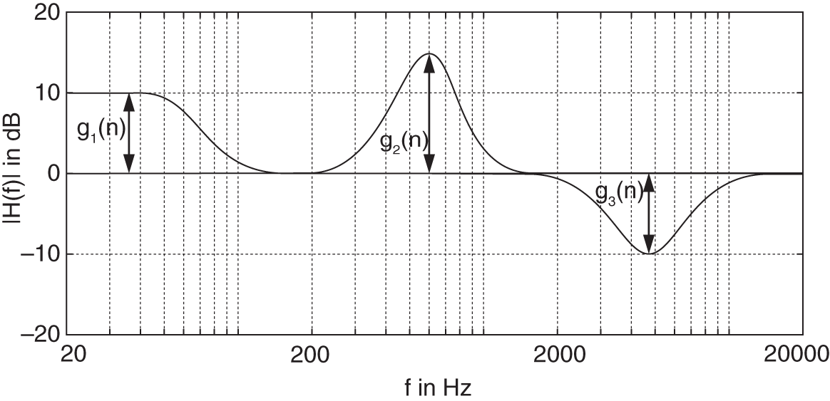
Figure 8.25 Frequency response of a dynamic equalizer at sample  .
.
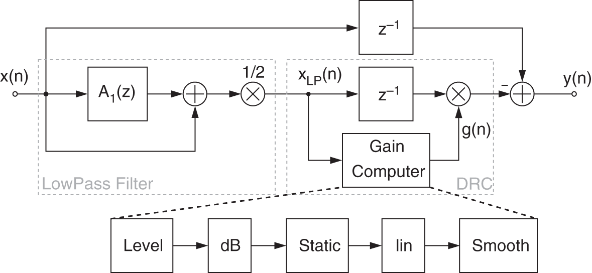
Figure 8.26 Block diagram of a low‐shelving dynamic filter.
A further approach, shown in Figs. 8.26 and 8.27, implements a dynamic shelving and peak filter based on an allpass filter decomposition for parametric equalization [Zöl08]. This implementation takes advantage of the lowpass and bandpass signal generated at the first stage to compute the level used later at the DRC stage.

Figure 8.27 Block diagram of a peak dynamic filter.
8.8 Source‐filter DRC
8.8.1 Introduction
Source‐filter separation and processing [Arf11] has been extensively used to extract the so‐called spectral envelope (filter coefficients) and the source signal from an audio signal. When applying the spectral envelope to the source signal again, the filtering operation will perfectly reconstruct the original. In the case of a speech signal, the spectral envelope has the advantage to provide a good representation of its formants. The idea of using the extracted formants to re‐synthesize voice has been expressed for a long time in [Sla62] and is nowadays used in applications such as Vocoders [Nag09] or artificial speech models [Kad07].
The system proposed here will apply some dynamic processing on the error signal (source signal) to affect the re‐synthesized result. However, too drastic modifications of the source signal can generate artifacts at the re‐synthesis stage. One of the applications presented here aims to reduce background noise and is especially effective when applied to speech recordings.
Source‐filter separation [Arf11], as shown in Fig. 8.28, uses linear predictive coding and decoding (LPC) by generating a prediction ![]() of the input signal
of the input signal ![]() with an adaptive FIR filter
with an adaptive FIR filter ![]() of order
of order ![]() . This filter estimates a spectral envelope of the input
. This filter estimates a spectral envelope of the input ![]() . The difference between the predicted signal and the input is called the prediction error
. The difference between the predicted signal and the input is called the prediction error ![]() and represents the source signal. The prediction error
and represents the source signal. The prediction error ![]() can be seen as a whitened version of
can be seen as a whitened version of ![]() . For speech signals, the prediction error (source signal) represents an excitation signal similar to the sound emitted by the vocal cords, which will be filtered by the vocal tract to give the spectral shape of the speech signal. Further dynamic range processing of the prediction error will lead to a processed source/error
. For speech signals, the prediction error (source signal) represents an excitation signal similar to the sound emitted by the vocal cords, which will be filtered by the vocal tract to give the spectral shape of the speech signal. Further dynamic range processing of the prediction error will lead to a processed source/error ![]() , which is then fed to the LPC decoding as shown in Fig. 8.28 to reconstruct the processed output
, which is then fed to the LPC decoding as shown in Fig. 8.28 to reconstruct the processed output ![]() .
.
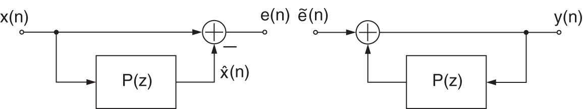
Figure 8.28 Source‐filter separation and processing using linear predictive coding (analysis) and decoding (synthesis).
The prediction filter ![]() of order
of order ![]() used in the analysis and synthesis is updated at every new incoming sample using a buffer of the
used in the analysis and synthesis is updated at every new incoming sample using a buffer of the ![]() past samples from
past samples from ![]() . The filter coefficients
. The filter coefficients ![]() are updated according to the least‐mean‐square (LMS) method given by
are updated according to the least‐mean‐square (LMS) method given by
for ![]() , where
, where ![]() is the filter coefficient index and
is the filter coefficient index and ![]() corresponds to the step size of the adaption. The predicted signal
corresponds to the step size of the adaption. The predicted signal ![]() is calculated using
is calculated using
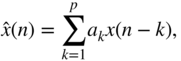
which represents FIR filtering of the input ![]() with the previously estimated filter coefficients. The transfer function for coding (analysis) is given by
with the previously estimated filter coefficients. The transfer function for coding (analysis) is given by
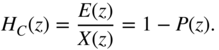
The decoder for the re‐synthesis uses the inverse transfer function of the coder given by
This filter uses the coefficients calculated by the prediction filter ![]() and performs as an all‐pole filter. From an implementation point of view, this is simply using the filter in a feedback loop, as depicted in Fig. 8.28.
and performs as an all‐pole filter. From an implementation point of view, this is simply using the filter in a feedback loop, as depicted in Fig. 8.28.
8.8.2 Combination with DRC
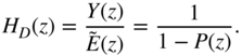
In this particular system, the error signal will be processed by a DRC system to influence the re‐synthesized signal ![]() , as depicted in Fig. 8.29. DRC produces generally a quite transparent effect. Therefore, the processed error signal will not be affected too drastically, so the reconstructed signal will be less prompt to artifacts arising from imperfect reconstruction.
, as depicted in Fig. 8.29. DRC produces generally a quite transparent effect. Therefore, the processed error signal will not be affected too drastically, so the reconstructed signal will be less prompt to artifacts arising from imperfect reconstruction.
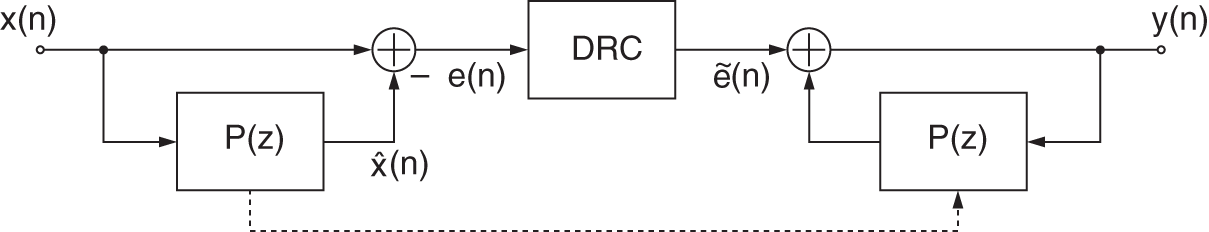
Figure 8.29 Block diagram of the combined systems LPC and DRC.
8.8.3 Applications
Denoising
Dynamic range control has been one of the first tools used to denoise audio signals. As an example, a noise gate or expander attenuates the input signal when its level goes below a defined threshold. By setting this threshold right above the background noise level, the parts where no signal of interest is present will see their level reduced, thus denoised. This denoising method is, by definition, effective only when the energy of the input signal is low in the case of a speech signal when the speaker is not speaking or pausing between words.
Figure 8.30 Error signals  and
and  before and after dynamic range expansion, respectively.
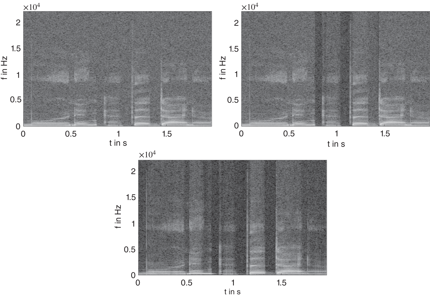
Figure 8.31 Spectrograms of a female singing voice with white noise (30 dB SNR; top left, input; top right, expanded input; bottom, denoised output).
In this denoising application, an expander is used as a DRC block, because it tends to be less prompt to artifacts than a noise gate. The expander chosen in this application is composed of a peak level detector [Gia12]. Because the error signal carries out most of the background noise, the expander threshold parameter can be set to a few dBs above the noise level (see Fig. 8.30). The pulse train remains, whereas the noise in between pulses is slightly reduced. Moreover, the silent part sees its background noise reduced as well, because the level is located below the expander threshold. For this application, the time constants of the expander have been set to a very fast attack ![]() ms to leave the transients and pulses untouched and a slower release
ms to leave the transients and pulses untouched and a slower release ![]() ms to avoid artifacts. A ratio
ms to avoid artifacts. A ratio ![]() has been chosen to drastically reduce the quieter sounds, thus the background noise. In this particular case, the threshold has been set up manually using prior knowledge of the noise level. However, an adaptive threshold may be applied for non‐stationary noise situations. It is worth mentioning that for high noise levels (that cover the speech), the presented algorithm will see its performances reduced drastically because its fundamental principle is to increase the level differences between parts of the signal. As mentioned in [Arf11], LPC can be parameterized so that the error signal resembles a whispering effect. This means that the resonant part of the voice is removed resulting in a combination of plosives, noise and pulse sequences. Removing the background noise from such a signal results in denoising the re‐synthesized signal. To obtain an excitation signal with such properties, filter orders in the range
has been chosen to drastically reduce the quieter sounds, thus the background noise. In this particular case, the threshold has been set up manually using prior knowledge of the noise level. However, an adaptive threshold may be applied for non‐stationary noise situations. It is worth mentioning that for high noise levels (that cover the speech), the presented algorithm will see its performances reduced drastically because its fundamental principle is to increase the level differences between parts of the signal. As mentioned in [Arf11], LPC can be parameterized so that the error signal resembles a whispering effect. This means that the resonant part of the voice is removed resulting in a combination of plosives, noise and pulse sequences. Removing the background noise from such a signal results in denoising the re‐synthesized signal. To obtain an excitation signal with such properties, filter orders in the range ![]() are most suitable (with
are most suitable (with ![]() kHz).
kHz).
The top left plot in Fig. 8.31 shows the spectrogram of a female singing voice with white noise (30 dB SNR). The top right plot spectrogram in Fig. 8.31 shows the effect of an expander applied as denoiser. In the case of the presence of stationary low‐colored background noise in a signal, it will be contained in the error signal ![]() as well, as the separation by the LPC is whitening the signal. By denoising the error signal with an expander, the re‐synthesized signal
as well, as the separation by the LPC is whitening the signal. By denoising the error signal with an expander, the re‐synthesized signal ![]() will also be denoised in parts where voicing is happening. This effect is visible on the spectrogram shown in the lower plot of Fig. 8.31, where an attenuation of the background noise is occurring without altering the original signal.
will also be denoised in parts where voicing is happening. This effect is visible on the spectrogram shown in the lower plot of Fig. 8.31, where an attenuation of the background noise is occurring without altering the original signal.
Transient Control
The error signal obtained by the source–filter separation contains the transients of the original sound. Because transients are sudden burst of energy, the prediction filter is not fast enough to predict them. This arises from to the weighted update of the filter coefficients (![]() ). Moreover, transients are generally broadband. This character makes them prompt not to be modeled by the filter, and therefore are present in the error signal.
). Moreover, transients are generally broadband. This character makes them prompt not to be modeled by the filter, and therefore are present in the error signal.
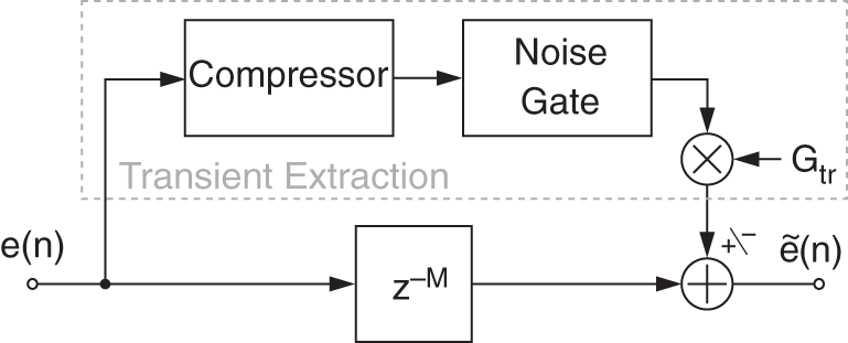
Figure 8.32 Block diagram of the DRC block for transient control.
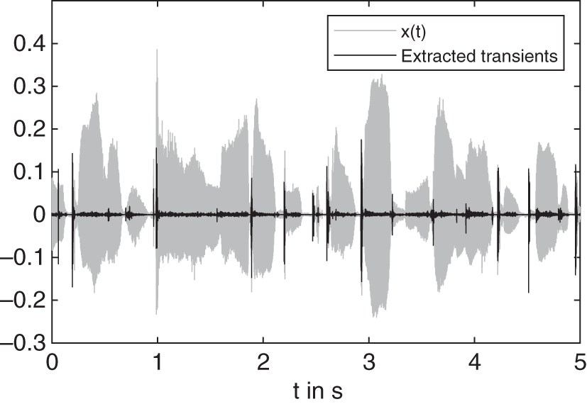
Figure 8.33 Input signal  and the corresponding extracted transients.
Once transients are extracted, it is possible to choose the amount to re‐inject into the error signal before the re‐synthesis. For this matter, a gain ![]() controlling the amount of transient to add or cancel (by phase inversion) is placed, as shown in Fig. 8.32. One of the problems occurring frequently when recording speech is the presence of too strong transients or clipping. This can arise from the air flow hitting the microphone membrane when pronouncing a plosive. Reducing transients may be used to reduce this effect (pop filtering). Traditionally, compressors are used to overcome such problems. Nevertheless, it is also considered that the attack portion of sounds conveys brightness character, so increasing the transients may also give a brighter effect to the re‐synthesized signal. Depending on the desired effect, being able to control the amount of transients in a sound is useful. This property makes the error a good pre‐processing step to extract transients. Processing it with a compressor can achieve a complete transient extraction.
controlling the amount of transient to add or cancel (by phase inversion) is placed, as shown in Fig. 8.32. One of the problems occurring frequently when recording speech is the presence of too strong transients or clipping. This can arise from the air flow hitting the microphone membrane when pronouncing a plosive. Reducing transients may be used to reduce this effect (pop filtering). Traditionally, compressors are used to overcome such problems. Nevertheless, it is also considered that the attack portion of sounds conveys brightness character, so increasing the transients may also give a brighter effect to the re‐synthesized signal. Depending on the desired effect, being able to control the amount of transients in a sound is useful. This property makes the error a good pre‐processing step to extract transients. Processing it with a compressor can achieve a complete transient extraction.
An example of extracted transients is shown in Fig. 8.33 and the corresponding spectrograms are visible in Fig. 8.34. Selecting a slower attack time will allow for the transient portion of the sound to pass through before the compressor starts clamping. However, if the attack time is too slow, then too big a portion of the transient may pass through. A noise gate is cascaded after the expander to fully remove the non‐transients parts (see Fig. 8.32).
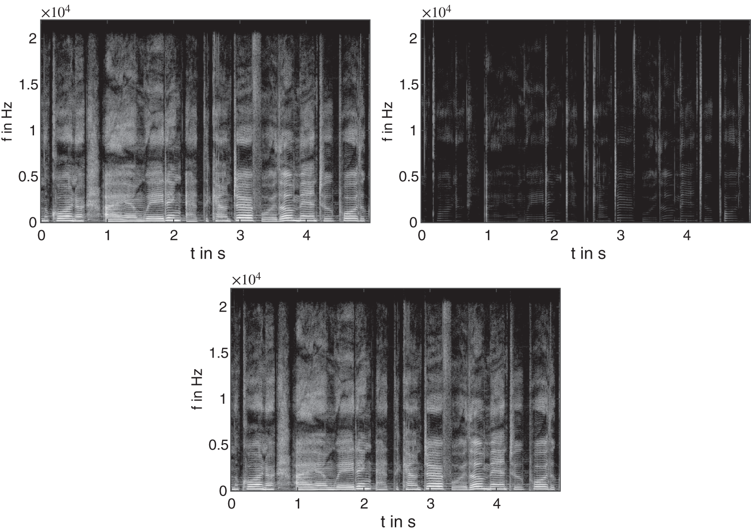
Figure 8.34 Spectrogram of a female singing voice (top left, input; top right, extracted transients; bottom, output with attenuated transients).
8.9 JS Applet – Dynamic Range Control
The applet shown in Fig. 8.35 demonstrates dynamic range control. It is designed for a first insight into the perceptual effects of dynamic range control of an audio signal. You can adjust the characteristic curve with two control points. You can choose between two predefined audio files from our web server (audio1.wav or audio2.wav) or your own local WAV file to be processed [Gui05].
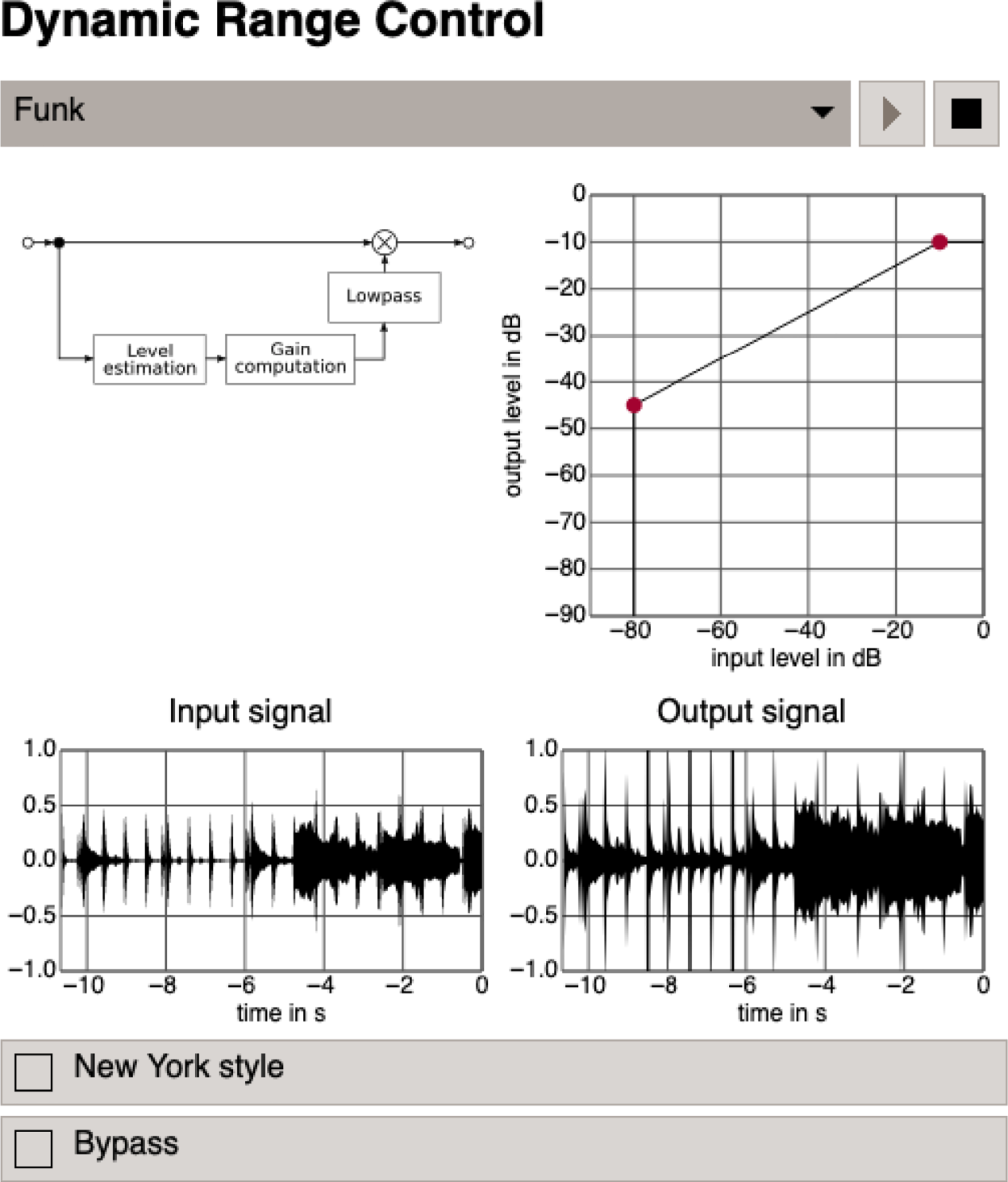
Figure 8.35 JS applet – dynamic range control.
8.10 Exercises
1. Lowpass Filtering for Envelope Detection
Generally, envelope computation is performed by lowpass filtering the input signal's absolute value or its square.
- Sketch the block diagram of a recursive first‐order lowpass
 .
. - Sketch its step response. What characteristic measure of the envelope detector can be derived from the step response and how?
- Typically, the lowpass filter is modified to use a non‐constant filter coefficient
 . How does
  depend on the signal? Sketch the response to a rect‐signal of the lowpass filter thus modified.
2. Discrete‐time Specialties of Envelope Detection
Taking absolute value or squaring are nonlinear operations. Hence care must be taken when using them in discrete‐time systems as they introduce harmonics the frequency of which may violate the Nyquist bound. This can lead to unexpected results, as a simple example shall illustrate. Consider the input signal ![]() .
.
- Sketch
 , and
, and  for different values of
  .
. - Determine the value of the envelope after perfect lowpass filtering, i.e. averaging,
 . Note: As the input signal is periodical, it is sufficient to consider one period, e.g.
- Similarly, determine the value of the envelope after averaging
 .
.
3. Dynamic Range Processors
Sketch the characteristic curves mapping input level to output level and input level to gain for, and describe briefly the application of:
- limiter;
- compressor;
- expander; and
- noise gate.
References
- [Arf11] D. Arfib, F. Keiler, U. Zölzer, and V. Verfaille: Source‐Filter Processing, chapter 8, pages 279–320. John Wiley and Sons, Ltd, 2011.
- [Dut11] P. Dutilleux, K. Dempwolf, M. Holters, and U. Zölzer: Nonlinear Processing, chapter 4, pages 101–138. John Wiley and Sons, Ltd, 2011.
- [Gia12] D. Giannoulis, M. Massberg, and J.D. Reiss: Digital dynamic range compressor design ‐ a tutorial and analysis. Journal of the Audio Engineering Society, 60(6):399–408, 2012.
- [Gui05] M. Guillemard, C. Ruwwe, U. Zölzer: J‐DAFx ‐ Digital Audio Effects in Java, Proc. 8th Int. Conference on Digital Audio Effects (DAFx‐05), Madrid, Spain, pp.161–166, 2005.
- [Kad07] Manjunath D. Kadaba: Artificial speech synthesis using LPC In Audio Engineering Society Convention 122, May 2007.
- [McN84] G.W. McNally: Dynamic Range Control of Digital Audio Signals, J. Audio Eng. Soc., Vol. 32, No. 5, pp. 316–327, 1984.
- [Nag09] F. Nagel, S. Disch, and N. Rettelbach: A phase vocoder driven bandwidth extension method with novel transient handling for audio codecs. In Audio Engineering Society Convention 126, May 2009.
- [Sla62] F.H. Slaymaker and R.A. Houde. Speech compression by analysis‐synthesis. J. Audio Eng. Soc, 10(2):144–148, 1962.
- [Sti86] E. Stikvoort: Digital Dynamic Range Compressor for Audio, J. Audio Eng. Soc., Vol. 34, No. 1/2, pp. 3–9, 1986.
- [Väl16] V. Välimäki and J.D. Reiss: All about audio equalization: Solutions and frontiers. Applied Sciences, 6(5), 2016.
- [Wis09] D.K. Wise: Concept, design, and implementation of a general dynamic parametric equalizer. Journal of the Audio Engineering Society, 57(1/2):1–28, January 2009.
- [Zöl08] U. Zölzer: Digital Audio Signal Processing. John Willey and Sons, 2008.