
Chapter 10
Nonlinear Processing
M. Holters and L. Köper
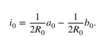
10.1 Fundamentals
Linear systems—filters—play an important role in audio signal processing. Linearity here means that the superposition property holds: denote the output of a system excited with input signals ![]() and
and ![]() with
with ![]() and
and ![]() , respectively. If the system maps the superposition of the input signals
, respectively. If the system maps the superposition of the input signals ![]() to the corresponding superposition
to the corresponding superposition ![]() at the output (for any
at the output (for any ![]() ), it is considered linear. Systems that do not fulfill this property are accordingly called nonlinear. One important consequence of linearity, when combined with time invariance, is that systems can be fully described in the frequency domain by their transfer function. Therefore, frequency components present in the input signal can be amplified or attenuated and phase‐shifted, but no new components can appear in the output. This is not the case for nonlinear systems, where in particular, components at multiples of the input frequency (harmonics) can appear. Figure 10.1 visualizes this important difference.
), it is considered linear. Systems that do not fulfill this property are accordingly called nonlinear. One important consequence of linearity, when combined with time invariance, is that systems can be fully described in the frequency domain by their transfer function. Therefore, frequency components present in the input signal can be amplified or attenuated and phase‐shifted, but no new components can appear in the output. This is not the case for nonlinear systems, where in particular, components at multiples of the input frequency (harmonics) can appear. Figure 10.1 visualizes this important difference.
We have already seen nonlinear systems, namely the dynamic range controllers of Chapter 8. However, when only considering short time spans (in relation to the attack and release times), they can be approximated by simply scaling the signal, a linear operation. This chapter, however, will focus on nonlinear systems where such an approximation is not fruitful.
An important distinction between nonlinear systems is whether they only act on the current input signal value (static, memoryless, or stateless system) or also contain an internal state (dynamic or stateful system). The latter can exhibit arbitrary behavior, while the former are more restricted and allow some general observations. We therefore first focus on static nonlinear systems.
A static nonlinear system can be described by a single function ![]() mapping input to output by
mapping input to output by
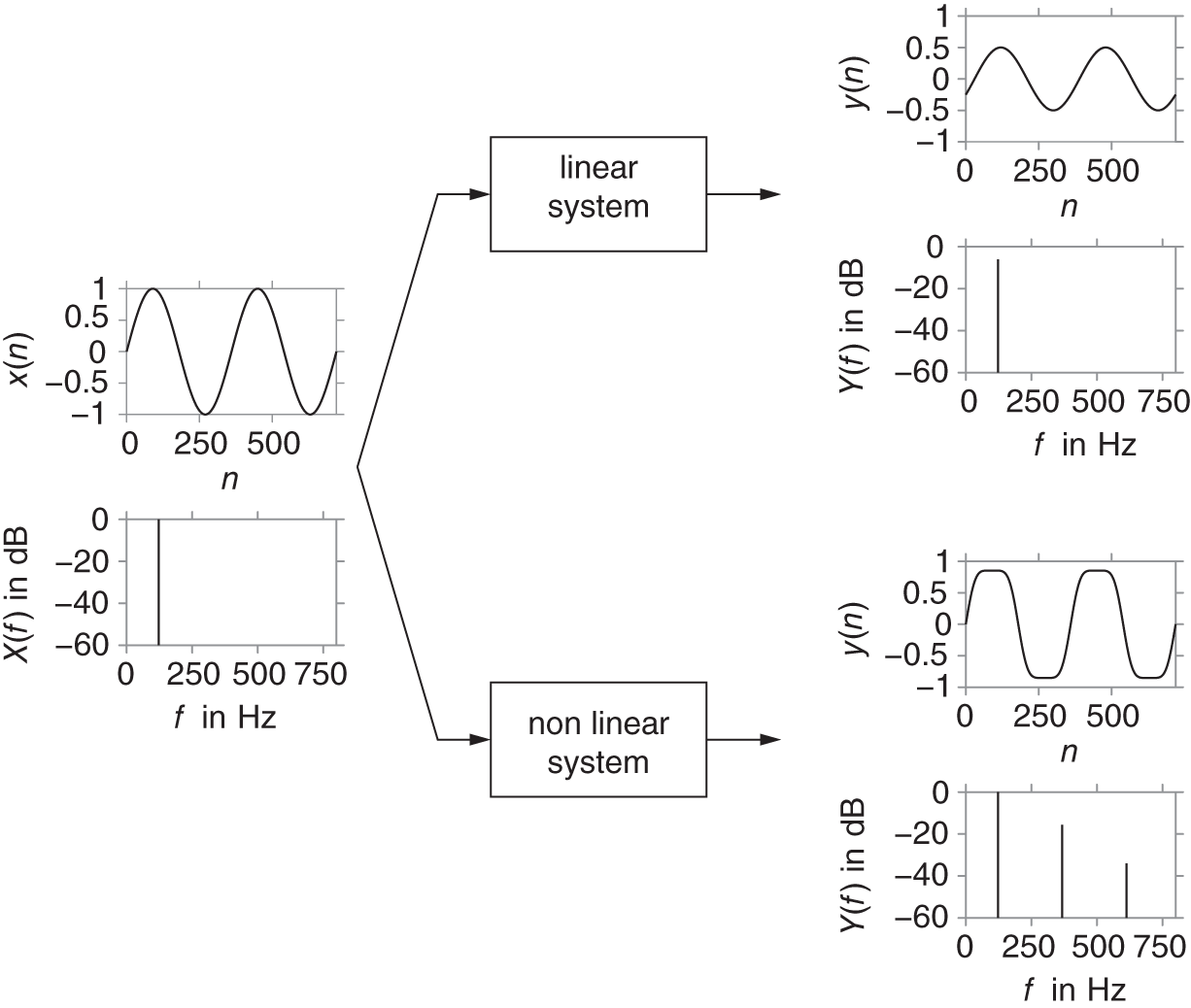
Figure 10.1 Comparison of a linear system and a nonlinear system when excited with a single sinusoid.
Now obviously, if ![]() is periodic with period
is periodic with period ![]() , then so is
, then so is ![]() . In particular, for a sinusoidal input
. In particular, for a sinusoidal input ![]() of frequency
of frequency ![]() , because the output
, because the output ![]() has period
has period ![]() , from Fourier theory we obtain that it can be decomposed as
, from Fourier theory we obtain that it can be decomposed as
i.e. it consists of sinusoids at multiples of the input frequency ![]() . While the DC component
. While the DC component ![]() is usually ignored, the component at
is usually ignored, the component at ![]() is referred to as the fundamental and the remaining components are called its harmonics.
is referred to as the fundamental and the remaining components are called its harmonics.
In contexts where a linear system is desired, the effect of a nonlinearity is therefore also called harmonic distortion. It is commonly measured by the total harmonic distortion (THD)
the ratio of the combined power of all harmonics to the total signal power (without the DC component). Usually, the THD is given in dB. While it quantifies the deviation from linearity for systems that should ideally be linear, it is of little use to characterize systems which are intentionally nonlinear, as the relative levels of the different harmonics have a strong influence on the resulting timbre.
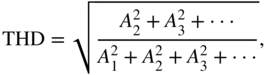
Typical audio signals of interest comprise more than a single sinusoid. Single note tones of musical instruments consist of a fundamental and its harmonics themselves. Any new components introduced by a static nonlinear system will still be harmonics, so the tonal quality remains, the appearance of new harmonics or amplification of existing ones will only make the sound brighter or even harsher. For input signals containing more than a single sinusoid and its harmonics, however, additional components appear spaced by the differences of the input signal frequencies. An example is given in Fig. 10.2, where the same static nonlinear system is excited with a single sinusoid at 261.63 Hz (C4, top), two sinusoids at 261.63 Hz and 392 Hz (C4 and G4, middle), and 261.63 Hz, 329.63 Hz and 392 Hz (C4, E4, and G4, i.e. Cmajor, bottom). As is apparent, additional components in the input signal quickly yield a very dense output spectrum. For that reason, intentional nonlinear processing is usually limited to single notes or chords with very few notes (e.g. power chords on an electric guitar).
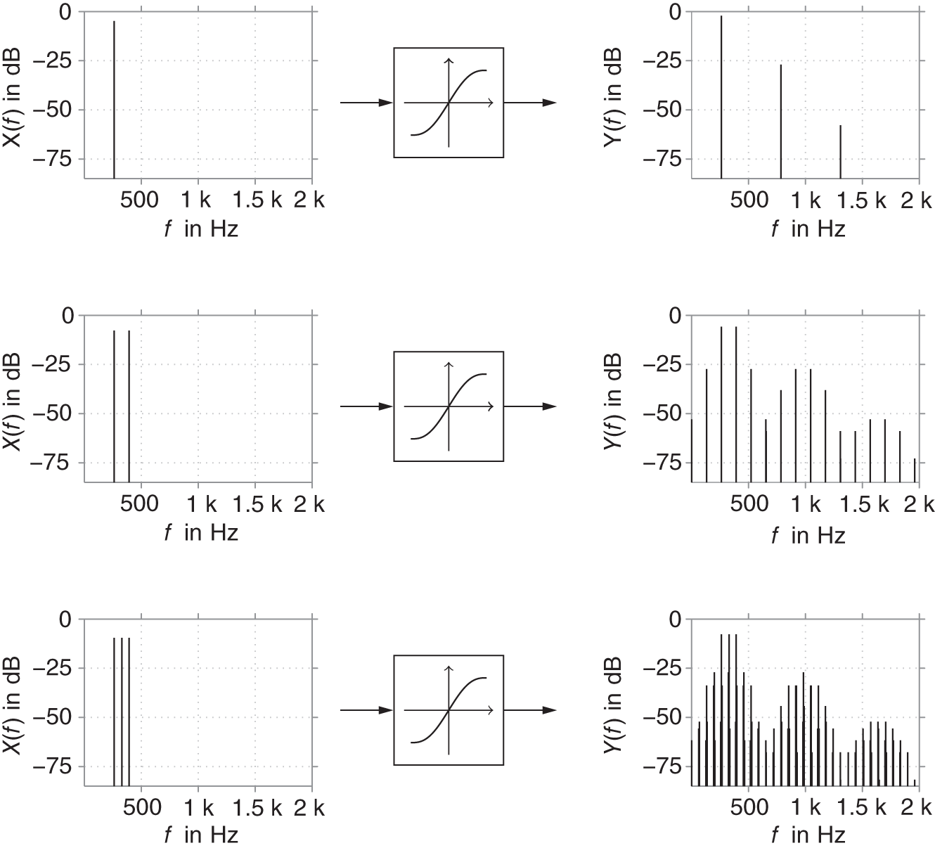
Figure 10.2 Effect of a static nonlinearity on a single sinusoid, two sinusoids, and three sinusoids.
10.2 Overdrive, Distortion, Clipping
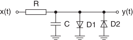
Overdrive, distortion, and clipping effects are heavily used in many kinds of musical devices. The terms overdrive and distortion are by no means exactly defined. However, most musicians will agree by defining overdrive as a soft saturating amplification of low‐level signals, which results in an operating point in the linear as well as nonlinear regions of the characteristic curve of the overdrive. A distortion effect will mainly be used in its nonlinear region. This leads to a harsher sound with a lot of harmonic frequency content. To design and analyze such effects, an understanding of the underlying nonlinear processing is crucial. A very basic clipping circuit can be obtained by connecting antiparallel diodes to the signal path. Figure 10.3 illustrates a soft‐clipping lowpass filter using only two additional diodes.
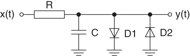
Figure 10.3 First‐order diode clipper.
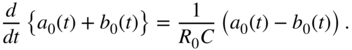
By disregarding the diodes, the transfer function of the linear lowpass filter can simply be found to be
with the corresponding differential equation
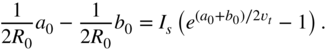
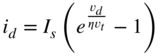
However, including the nonlinearity, which is introduced by the diodes, to the transfer function is not straightforward. The nonlinear relation of the voltage over and the current through the diode can be obtained using Shockley's law:
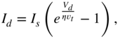
with ![]() as the current through,
as the current through, ![]() the voltage over the diode,
the voltage over the diode, ![]() as the reverse saturation current,
as the reverse saturation current, ![]() as thermal voltage, and
as thermal voltage, and ![]() as quality factor. Applying Kirchoff's voltage and current laws to the circuit from Fig. 10.3 and assuming identical diodes, a first‐order nonlinear differential equation,
as quality factor. Applying Kirchoff's voltage and current laws to the circuit from Fig. 10.3 and assuming identical diodes, a first‐order nonlinear differential equation,
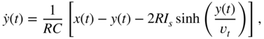
can be derived.
Although this equation describes the system in its entirety, implementing it into a digital processing unit cannot be done easily, because the nonlinear differential equation needs to be solved numerically for each and every time step. This computational effort even increases for more complicated systems. Hence, the question arises whether the system can be somehow separated into a linear and a nonlinear part. Looking at the system from Fig. 10.3, the most intuitive idea is to apply first a linear lowpass filter and afterwards a nonlinear mapping function. Figure 10.4 shows such a system. The discrete input signal ![]() is filtered by a linear lowpass filter and afterwards fed into the nonlinearity. Note that this separation into a linear stateful filter and a static nonlinear mapping function does not perfectly recreate the dynamic behavior of nonlinear stateful filters such as in Eq. (10.7). However, many nonlinear systems can be sufficiently approximated by approaches based on Fig. 10.4.
is filtered by a linear lowpass filter and afterwards fed into the nonlinearity. Note that this separation into a linear stateful filter and a static nonlinear mapping function does not perfectly recreate the dynamic behavior of nonlinear stateful filters such as in Eq. (10.7). However, many nonlinear systems can be sufficiently approximated by approaches based on Fig. 10.4.
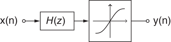
Figure 10.4 Combination of linear filtering and nonlinear static mapping.
As shown for the simple example in Fig. 10.3, nonlinear processing of such dynamic systems is very tedious. Hence, we will focus on the use of static nonlinear mapping functions to create overdrive and distortion effects. A simple soft clipping characteristic curve [Sche80] is given by the equation
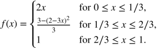
A corresponding hard clipping characteristic curve
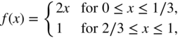
can be obtained by removing the quadratic term from the soft‐clipping equation. Figure 10.5 shows both soft‐ and hard clipping mapping functions corresponding to Eq. (10.8) and Eq. (10.9) in symmetrical application ![]() for
for ![]() . The output signal for such a system given a sinusoidal input of 1 kHz and an amplitude of 0.8 V is depicted in Fig. 10.6. Applying such symmetrical nonlinear functions to a sinusoidal input signal resolves into an output signal which contains only odd harmonics of the original signal. Furthermore, hard clipping nonlinearities will produce a higher harmonic frequency content compared with the smoother soft‐clipping nonlinearity. However, if the characteristic curve is asymmetric, e.g. Eq. (10.8) with
. The output signal for such a system given a sinusoidal input of 1 kHz and an amplitude of 0.8 V is depicted in Fig. 10.6. Applying such symmetrical nonlinear functions to a sinusoidal input signal resolves into an output signal which contains only odd harmonics of the original signal. Furthermore, hard clipping nonlinearities will produce a higher harmonic frequency content compared with the smoother soft‐clipping nonlinearity. However, if the characteristic curve is asymmetric, e.g. Eq. (10.8) with ![]() for
for ![]() , the output signal will contain both even and odd harmonics. Stateful nonlinear filters might also add non‐harmonic frequency content to the signal. This is, for example, the case if looking at self‐oscillating systems.
, the output signal will contain both even and odd harmonics. Stateful nonlinear filters might also add non‐harmonic frequency content to the signal. This is, for example, the case if looking at self‐oscillating systems.
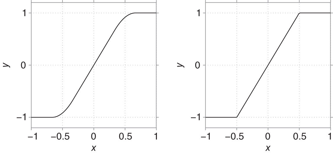
Figure 10.5 Static characteristic curve of a symmetrical soft‐clipping (left) and hard clipping (right) nonlinearity.
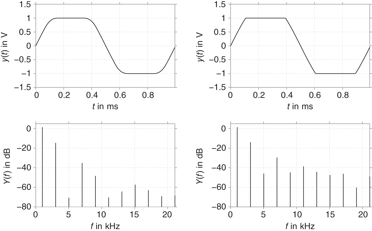
Figure 10.6 Output signal for sinusoidal input with soft‐clipping (left) and hard clipping (right) nonlinearity.
Another nonlinear processing technique similar to clipping is called wavefolding. It also uses a nonlinear static mapping function, but instead of saturating the input signal, some parts of the input signal are folded back onto itself. The name wavefolding has its origin in the early days of electronic sound synthesis. A wavefolder takes a sine or cosine wave as an input and produces an output wave with high harmonic frequency content [Roa79]. The wavefolding process is depicted in Fig. 10.7. Using the upper linear mapping function, the signal can be inverted. Applying this inversion only to certain parts of the input signal results in an output signal similar to that shown at the bottom of Fig. 10.7. The resulting output signal has a high amount of harmonic frequency content. Because the input signal to such wavefolders is typically a sinusoid with no harmonic frequency content, this technique is often used for additive synthesis.
Figure 10.7 Wavefolding using nonlinear static mapping functions.
10.3 Nonlinear Filters
Describing nonlinear systems as a combination of linear filters and static nonlinear mapping functions is sufficient for many applications. However, sometimes it is necessary to implement the nonlinearities directly into the filter, which results in a stateful nonlinear filter. For example, by adding saturating nonlinearities, a digital filter can be constructed that has a more ‘analog’‐like sound [Ros92]. The stability of these nonlinear systems cannot be as easily determined as for linear systems. We have to take into account the fact that the pole locations are now dependent on the state of the filter. Therefore, stability analysis will make use of the instantaneous pole locations of the filter. We will investigate a stateful nonlinear filter by looking at a second‐order filter [Cho20], as depicted in Fig. 10.8. The difference equation for the output can be directly constructed from the block diagram with
Transforming the difference equation into the frequency domain, the transfer function
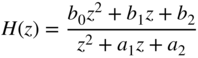
is obtained. This leads to the pole locations
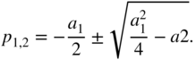
For further analysis, it is helpful to bring the system into a state‐space representation. Therefore we define the states to be the outputs of the delay blocks. This leads to the discrete‐time state‐space system:
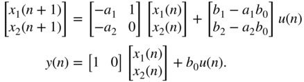
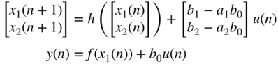
Note that the stability of this linear system requires all eigenvalues of the system matrix to have a magnitude smaller than one. A nonlinear version of this filter can be achieved by inserting nonlinear mapping functions, as mentioned in Section 10.2, into the filter. The nonlinear blocks are put directly behind the delay blocks. The output equation changes to
The nonlinear state‐space model results in
with
Because the poles of this nonlinear system are dependent on the state of the system, stability can be analyzed by looking at the instantaneous pole locations of the filter. Stability can be assured if all possible instantaneous pole locations have a magnitude strictly smaller than one. Therefore, the Lyapunov stability [Che04] of the system can be analyzed. Note that the Lyapunov stability is more restrictive than the BIBO stability, because a Lyapunov stable system will only have poles inside the unit circle for any given point in time. A system is considered Lyapunov stable if the eigenvalues for the Jacobian of the discrete‐time system matrix have magnitudes strictly smaller than one. The Jacobian of the nonlinear state‐space system yields
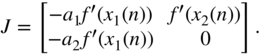
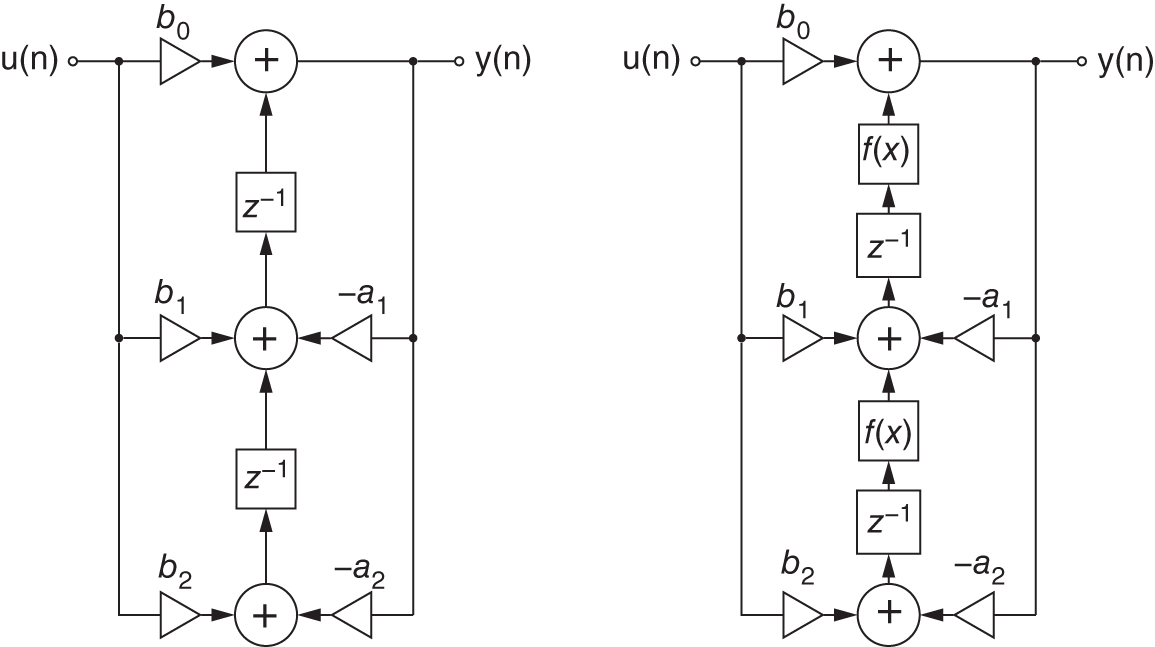
Figure 10.8 Linear (left) and nonlinear (right) second‐order filter.
Consequently, there are two restrictions for the system to be stable. The backward coefficients have the same restriction as for the linear system with ![]() for real poles and
for real poles and ![]() for conjugate complex poles. Furthermore, the first derivative of the nonlinear mapping function must not exceed a value of one at all operating points. Many nonlinear saturating functions fulfill this requirement. For example, a hyperbolic tangent, as in Fig. 10.9, can be used.
for conjugate complex poles. Furthermore, the first derivative of the nonlinear mapping function must not exceed a value of one at all operating points. Many nonlinear saturating functions fulfill this requirement. For example, a hyperbolic tangent, as in Fig. 10.9, can be used.
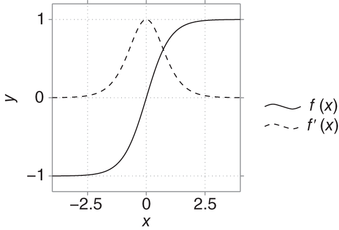
Figure 10.9 Hyperbolic tangent mapping function.
To illustrate the characteristics of such nonlinear filters, we take the second‐order filter from Fig. 10.8 as an example. The filter coefficients are set to ![]() ,
, ![]() ,
, ![]() , and
, and ![]() , which results in a lowpass configuration of the filter. The frequency response of the linear filter can be seen in Fig. 10.10. In this example, we will use a linear sinesweep with amplitude 1 and a frequency range from
, which results in a lowpass configuration of the filter. The frequency response of the linear filter can be seen in Fig. 10.10. In this example, we will use a linear sinesweep with amplitude 1 and a frequency range from ![]() to
to ![]() as an input signal to the filters. The output signal over time and frequency can be seen in the waterfall representations shown in Fig. 10.11 and Fig. 10.12. The lowpass behavior of the filters can be observed in both figures because the higher frequencies of the sinesweep receive a higher attenuation. The nonlinear filter additionally produces filtered harmonics of the input signal. This feature can be used to create sounds with a more analog‐like feel like saturated transistor or tube stages.
as an input signal to the filters. The output signal over time and frequency can be seen in the waterfall representations shown in Fig. 10.11 and Fig. 10.12. The lowpass behavior of the filters can be observed in both figures because the higher frequencies of the sinesweep receive a higher attenuation. The nonlinear filter additionally produces filtered harmonics of the input signal. This feature can be used to create sounds with a more analog‐like feel like saturated transistor or tube stages.
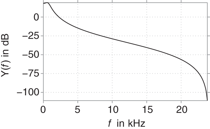
Figure 10.10 Frequency response of linear second‐order filter.
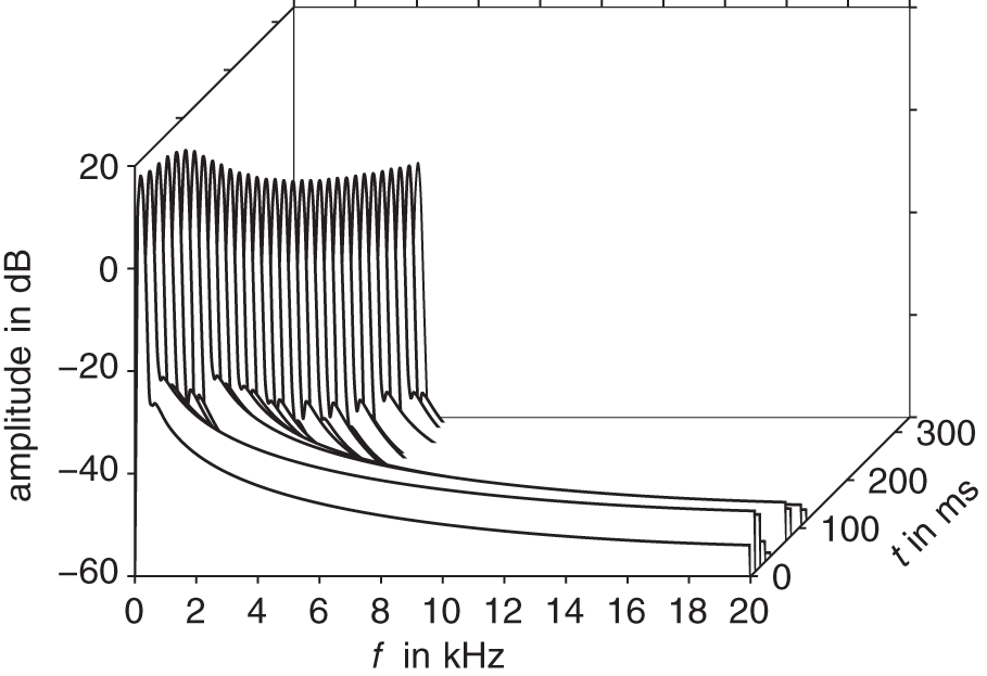
Figure 10.11 Waterfall presentation of a linear filtered sinesweep.
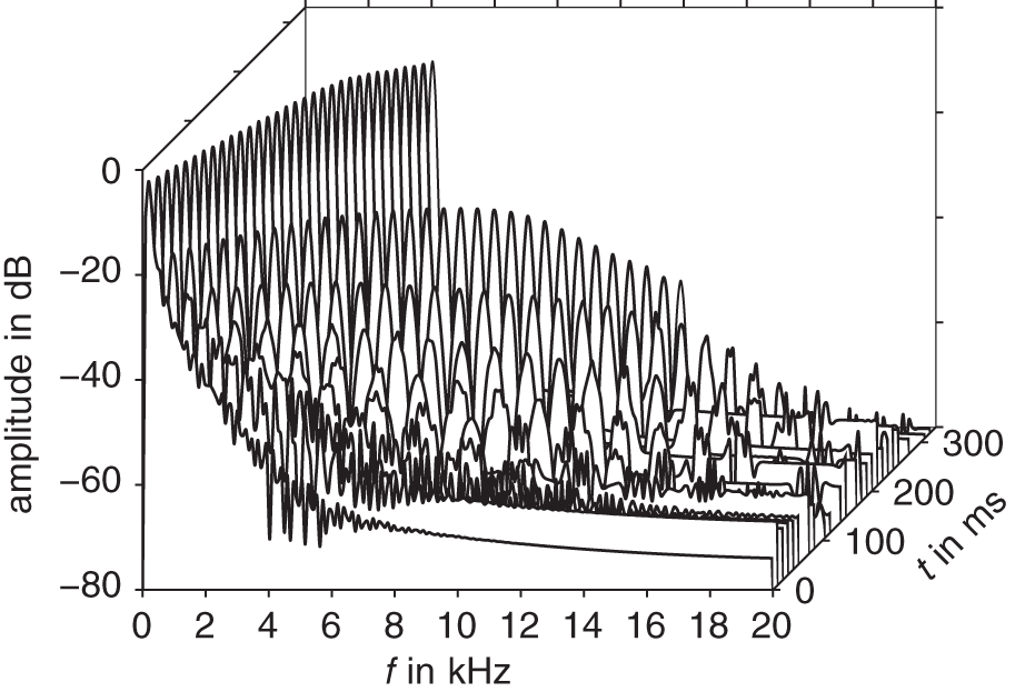
Figure 10.12 Waterfall presentation of a nonlinear filtered sinesweep.
10.4 Aliasing and its Mitigation
So far, we have ignored one important aspect of nonlinear processing: the newly introduced signal components, especially higher harmonics, may exceed the Nyquist limit at half the sampling frequency. This will result in aliasing distortion, which is typically undesired. We may first observe that when considering a continuous‐time input signal ![]() , the order of sampling and applying a static nonlinear mapping
, the order of sampling and applying a static nonlinear mapping ![]() may be reversed: First applying
may be reversed: First applying ![]() gives
gives ![]() , which, after sampling with sampling rate
, which, after sampling with sampling rate ![]() , results in
, results in ![]() . However, by first sampling, we get
. However, by first sampling, we get ![]() , which is then mapped to the same
, which is then mapped to the same ![]() . This holds true even if
. This holds true even if ![]() is not band limited to
is not band limited to ![]() .
.
As an extreme case, we consider the mapping function ![]() , which corresponds to applying an infinite gain and then hard clipping to the range
, which corresponds to applying an infinite gain and then hard clipping to the range ![]() . Applied to a sinusoidal input, the output becomes a square wave. Figure 10.13a depicts the corresponding spectrum for an input frequency of 1318.5 Hz (the note E6). As the harmonics only decay slowly with frequency, their level above the Nyquist limit of 22.05 kHz (marked by a vertical line) for the common sampling rate of
. Applied to a sinusoidal input, the output becomes a square wave. Figure 10.13a depicts the corresponding spectrum for an input frequency of 1318.5 Hz (the note E6). As the harmonics only decay slowly with frequency, their level above the Nyquist limit of 22.05 kHz (marked by a vertical line) for the common sampling rate of ![]() is still significant. Consequently, the sampled signal of Fig. 10.13b contains many and strong aliased components. These will be audible as both a noise floor and inharmonic tones.
is still significant. Consequently, the sampled signal of Fig. 10.13b contains many and strong aliased components. These will be audible as both a noise floor and inharmonic tones.
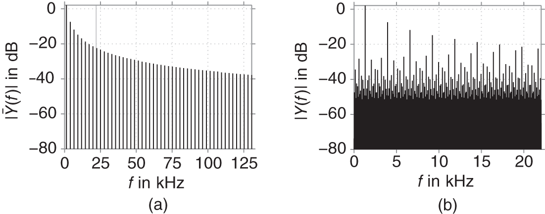
Figure 10.13 Spectra of (a) continuous‐time signal  with a marker at the Nyquist frequency 22.05 kHz and (b) sampled signal
 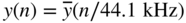 .
.
The conceptually simplest approach to reducing this aliasing distortion is to increase the sampling rate. Typically, the input signal will be upsampled before and downsampled to the original sampling rate after the nonlinearity, where the resampling includes appropriate interpolation and decimation filters. A corresponding system is shown in Fig. 10.14. The effectiveness of this method depends on how fast the harmonics decay with frequency and obviously the oversampling factor ![]() . For the example above, the spectra obtained by oversampling with different factors
. For the example above, the spectra obtained by oversampling with different factors ![]() are shown in Fig. 10.15.
are shown in Fig. 10.15.
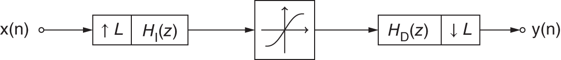
Figure 10.14 Operation of a nonlinear system at a sampling frequency increased by factor  , where
  and
and  denote the interpolation and decimation filter, respectively.
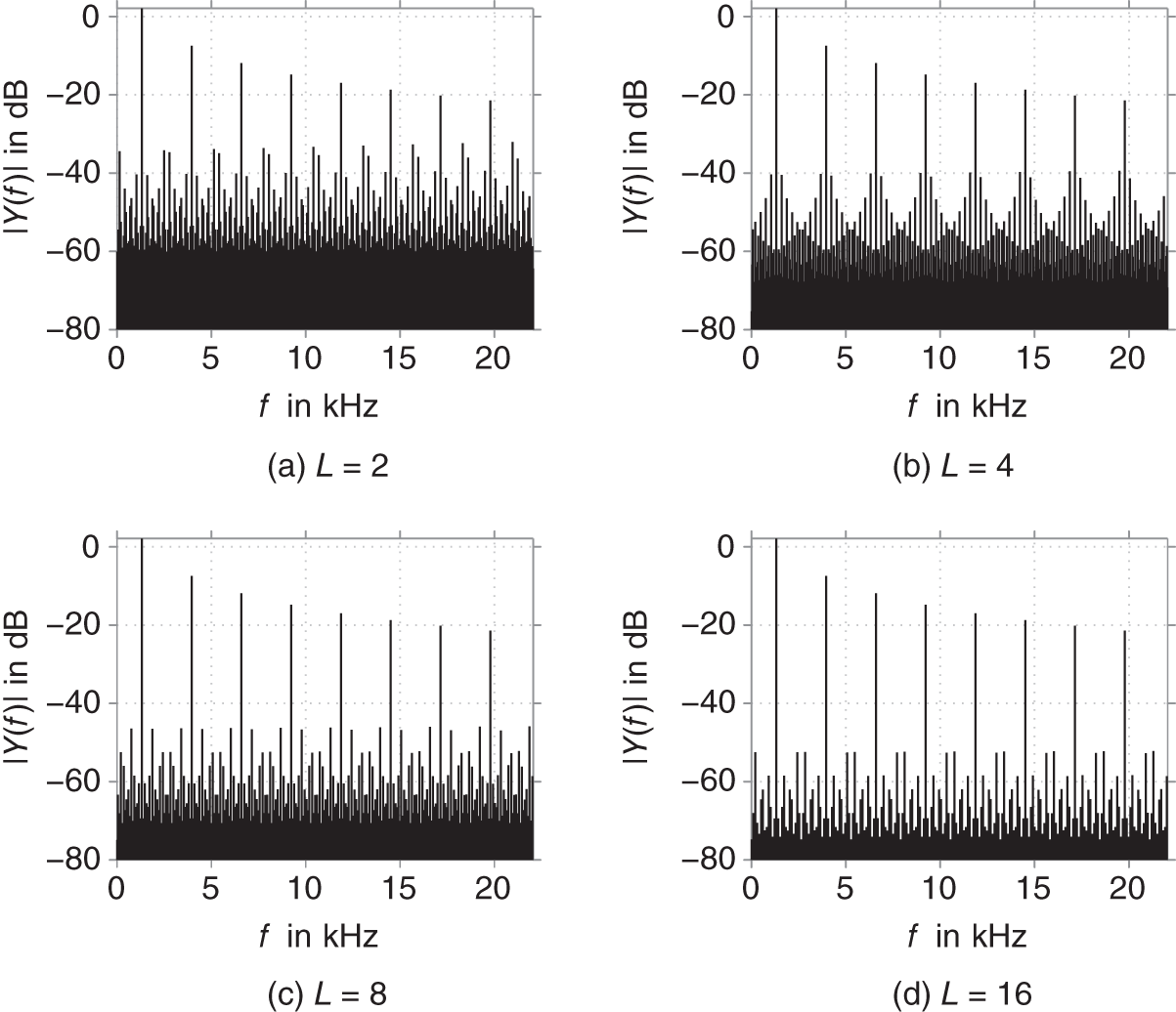
Figure 10.15 Spectra of  for different values of
  .
.
It is clearly visible that with increasing ![]() , the aliasing distortion gets reduced. For less extreme nonlinear systems, the harmonics typically decay faster and the effect of oversampling will be even more pronounced.
, the aliasing distortion gets reduced. For less extreme nonlinear systems, the harmonics typically decay faster and the effect of oversampling will be even more pronounced.
However, owing to increasing computational costs, the oversampling factor usually cannot be made arbitrarily large. Therefore, various other strategies to reduce the aliasing distortion have been developed, e.g. [Esq15, Esq16a, Esq16b, Mul17]. In the case of a memoryless nonlinear system, an attractive approach is based on approximating a continuous‐time system [Par16, Bil17a, Bil17b], which will be explained in the following. Perfect aliasing suppression can be obtained by carrying out the processing in the continuous‐time domain, i.e. by converting the input signal to its continuous representation, applying the nonlinearity to it, and then sampling it after appropriate lowpass filtering. While theoretically perfect, this is clearly impractical. However, by crude approximation of this process, we can obtain a practical implementation that can considerably lower the aliasing distortion.
First, we replace the exact continuous‐time representation of the input signal by a piecewise linear approximation:
To this we apply the nonlinear mapping to obtain
Before sampling this, we need to apply a lowpass to suppress frequency content above the Nyquist limit. In the simplest case, we average over one sampling interval (corresponding to convolution with a rect), i.e.
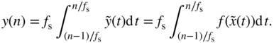
Now we apply integration by substitution and rewrite as
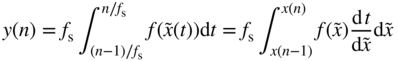
and exploit the fact that, thanks to the piecewise linear approximation,
is easy to compute. We thus obtain

Finally, by the fundamental theorem of calculus, we may rewrite to
where ![]() denotes the antiderivative of
denotes the antiderivative of ![]() . The method is therefore also referred to as antiderivative antialiasing. If the antiderivative cannot be derived in closed form, it can be precomputed numerically and tabulated.
. The method is therefore also referred to as antiderivative antialiasing. If the antiderivative cannot be derived in closed form, it can be precomputed numerically and tabulated.
Assuming evaluation of ![]() to be approximately as expensive as evaluation of
to be approximately as expensive as evaluation of ![]() and when memorizing
and when memorizing ![]() to be used as
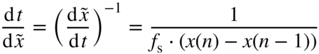
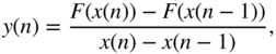
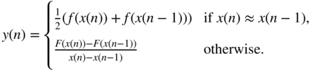
to be used as ![]() in the next time step, the antialiased system only requires two additional subtractions and one additional division compared with the non‐antialiased system. There is one minor complication though, namely, when
in the next time step, the antialiased system only requires two additional subtractions and one additional division compared with the non‐antialiased system. There is one minor complication though, namely, when ![]() , the denominator of Eq. (10.25) becomes nearly (or even exactly) zero, which will result in numerical problems. In the limit
, the denominator of Eq. (10.25) becomes nearly (or even exactly) zero, which will result in numerical problems. In the limit ![]() , Eq. (10.25) reduces to
, Eq. (10.25) reduces to ![]() or equally
or equally ![]() . Thus, one could use either of those in case
. Thus, one could use either of those in case ![]() , but as will be explained momentarily, their mean
, but as will be explained momentarily, their mean ![]() is the most consistent choice. So to summarize, antiderivative antialiasing is given by
is the most consistent choice. So to summarize, antiderivative antialiasing is given by
While the approach thus derived is attractive owing to its simplicity, the interpolation and decimation filters are far from the ideal brick‐wall filters. This will lead to both an unwanted lowpass filtering of the desired signal components and an imperfect suppression of the image spectra. To first analyze the unwanted lowpass filtering, we consider the effect of applying the antiderivative antialiasing to a linear system, choosing in particular ![]() . With
. With ![]() , we find
, we find
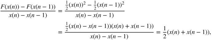
which equals our choice for the ![]() case, thereby justifying it. We notice that the antialiasing introduces a half‐sample delay and the expected lowpass filtering. Concerning the imperfect suppression of the image spectra, note that the frequency response of the rect filter has zeros at the multiples of the sampling rate
case, thereby justifying it. We notice that the antialiasing introduces a half‐sample delay and the expected lowpass filtering. Concerning the imperfect suppression of the image spectra, note that the frequency response of the rect filter has zeros at the multiples of the sampling rate ![]() , i.e. those components that would be aliased to DC are suppressed perfectly. Components that are aliased to low frequencies still see very high suppression. However, components just above the Nyquist limit are only attenuated by a meager 3 dB, leaving strong aliased components at high frequencies.
, i.e. those components that would be aliased to DC are suppressed perfectly. Components that are aliased to low frequencies still see very high suppression. However, components just above the Nyquist limit are only attenuated by a meager 3 dB, leaving strong aliased components at high frequencies.
These effects can be seen in Fig. 10.16a, where the same example of ![]() excited with a sine at 1318.5 Hz as before is now subject to antiderivative antialiasing. Compared with Fig. 10.13b, one clearly sees that the aliasing distortion at low frequencies is greatly reduced, while the strongest components at high frequencies see almost no reduction. At the same time, the desired signal components undergo a slight lowpass filtering, as can be seen from the comparison to their desired levels marked by crosses.
excited with a sine at 1318.5 Hz as before is now subject to antiderivative antialiasing. Compared with Fig. 10.13b, one clearly sees that the aliasing distortion at low frequencies is greatly reduced, while the strongest components at high frequencies see almost no reduction. At the same time, the desired signal components undergo a slight lowpass filtering, as can be seen from the comparison to their desired levels marked by crosses.
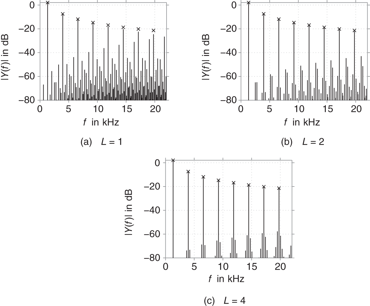
Figure 10.16 Spectra of output obtained with antiderivative antialiasing for different values of  , where crosses mark the desired harmonics.
As the antiderivative antialiasing works especially well at low frequencies, it is beneficial to combine it with oversampling to effectively broaden the frequency range of satisfactory aliasing suppression in addition to the aliasing reduction by the oversampling itself. The results obtained from two‐ and four‐times oversampling are shown in Fig. 10.16b and Fig. 10.16c. Compared with the case of oversampling alone (Fig. 10.15a and Fig. 10.15b), the effectiveness of antiderivative antialiasing is obvious.
While the piecewise linear interpolation is required to make the integration by substitution feasible in Eq. (10.22), alternatives for the decimation filter are possible. In [Par16], a tri filter is explored, while [Bil17a, Bil17b] view Eq. (10.25) as a discrete‐time approximation of differentiating the antiderivative ![]() and explore using higher‐order antiderivatives and different differentiation schemes. This allows to strike different balances between computational complexity, aliasing suppression, and alteration of the desired signal components.
and explore using higher‐order antiderivatives and different differentiation schemes. This allows to strike different balances between computational complexity, aliasing suppression, and alteration of the desired signal components.
Unfortunately, antiderivative antialiasing is only applicable to memoryless nonlinear systems. In [Hol20], an extension to a class of stateful systems is proposed. However, it is limited to systems which can be written in a particular way where all nonlinear functions only depend on a single scalar input. An alternative approach is discussed in [Mul17], where the system output is calculated not only based on the system state, but also its derviative, which enables an additional smoothing that can reduce aliasing. In particular, it can achieve high suppression of the harmonics around the sampling rate but has little effect on even higher harmonics. It is therefore mainly effective for nonlinear systems with relatively quickly decaying harmonics.
10.5 Virtual Analog Modeling
Constructing nonlinear systems directly in the digital domain is a sound and flexible method. However, oftentimes there is a need to create a digital model taken from existing analog circuits. The field of virtual analog modeling provides many different approaches and techniques for creating suitable digital models from analog reference circuits. There are a variety of different approaches, which all can be categorized into three different model types: blackbox models, graybox models, and whitebox models. A blackbox model is based solely on the input and output data of the analog circuit. In whitebox modeling approaches, all information regarding the analog circuit is known and can be used. This includes input and output data as well as voltage and current relations on each and every point in the circuit. A graybox model is something in between these two by having access to more information than just input and output data, but limited nonetheless. In this chapter, we will give a brief introduction of the most commonly used whitebox modeling approaches i.e. wave digital filters and state‐space modeling. Although we will not give a detailed analysis of the graybox and blackbox modeling approaches, we will provide a brief reference to some of the most used techniques. A commonly applied graybox modeling approach is the use of Wiener–Hammerstein models. These models divide the overall model into several linear and nonlinear parts. This approach is similar to that shown in Fig. 10.4, where we separated a nonlinear filter into a linear filter with a subsequent static nonlinearity. This and similar graybox modeling approaches are applied successfully in [Kem08, Eic16, Fra13]. In the domain of blackbox modeling, only input and output data are available for the model construction. To model such kinds of time‐series data, certain artificial neural network structures can be used. The most common one is the recurrent neural network, which is fruitfully used in [Wri19]. In [Par19], a neural network is combined with a whitebox state‐space modeling approach.
10.5.1 Wave Digital Filters
Wave digital filters can be used to transform an analog circuit from the Kirchhoff domain to the so‐called wave domain. This representation allows efficient and precise modeling of linear as well as nonlinear analog circuits. A circuit element is described in the wave domain by an incident and a reflected wave with a corresponding port resistance. A port is characterized by its port voltage ![]() and its port current
and its port current ![]() . The corresponding wave variables are constructed with a linear combination of port voltage and current with the port resistance as a parameter. The incident and reflected wave are defined as [Fet86]
. The corresponding wave variables are constructed with a linear combination of port voltage and current with the port resistance as a parameter. The incident and reflected wave are defined as [Fet86]
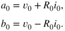
This can be written into matrix notation as
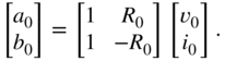
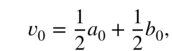
Solving now Eq. (10.29) for ![]() and
and ![]() , the port voltages and currents can respectively be obtained from the wave variables with
, the port voltages and currents can respectively be obtained from the wave variables with
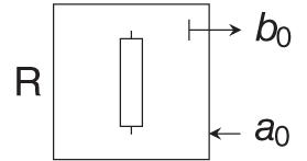
With these definitions, circuit elements can now be transformed from Kirchhoff to wave domain. Rather than covering all possible circuit elements in the wave domain, we restrict ourselves to the most common ones to give a brief overview and a basic understanding. We start with the simple example of transforming a resistor into the wave domain. A resistor is described in Kirchhoff domain by Ohm's law:
Combining this with Eq. (10.30a) and Eq. (10.30b) and solving for the reflected wave ![]() yields
yields

This is the so‐called unadapted form of a resistor in the wave domain. Most elements can be adapted by parameterizing the port resistance ![]() to a suitable value. In this case, we can set
to a suitable value. In this case, we can set ![]() and we obtain
and we obtain ![]() as the adapted form of a resistor in the wave domain [Wer16].
as the adapted form of a resistor in the wave domain [Wer16].
Similar to this derivation, we can obtain the wave‐domain representation of a capacitor. Starting with the differential equation
we can use (Eqs. 10.30a) and (10.30b) to obtain a differential equation depending on the wave variables with
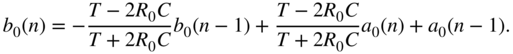
Going further, the continuous time differential equation needs to be discretized. Many discretization schemes might by used here, all with certain advantages and drawbacks. Here we choose one of the most common ones with the trapezoidal rule:
where ![]() is the corresponding differential equation and
is the corresponding differential equation and ![]() the sampling interval. After discretization with the trapezoidal rule, the difference equation for the reflected wave in the time domain yields [Wer16]
the sampling interval. After discretization with the trapezoidal rule, the difference equation for the reflected wave in the time domain yields [Wer16]
This unadapted form can be adapted as well by setting the port resistance to ![]() , which results in the adapted wave‐domain representation
, which results in the adapted wave‐domain representation
Note that instead of applying the trapezoidal rule in the time domain, we could also transform the differential equation to the frequency domain and use the bilinear transform for discretization, which will ultimately lead to the same result.
Other algebraic or reactive elements can be derived similarly. Table 10.1 comprises the wave‐domain representation of the most common linear circuit elements.
Table 10.1 Wave domain representation of common linear circuit elements
| Element | Port resistance | Wave equation |
|---|---|---|
 | ||
 | ||
 | ||
 | not adaptable | |
 | not adaptable |
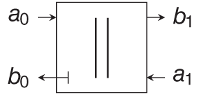
Table 10.2 Parallel and series adaptors
| Element | Port resistance | Wave equation |
|---|---|---|
 |  | |
 |  | |
 |  | |
 |  |
As an example for a nonlinear circuit element, we will derive a wave‐domain representation of a simple diode. An ideal diode can be described by Shockley's law given in Eq. (10.6). For the sake of simplicity, we will set the ideality factor to ![]() . Transforming Shockley's law into the wave domain, we obtain
. Transforming Shockley's law into the wave domain, we obtain
For use in a wave digital filter, the wave equation should be given in explicit form. However, owing to the exponential, Eq. (10.38) cannot be simply brought into an explicit formulation. Luckily we can bring Eq. (10.38) into a form which can be explicitly solved for the reflected wave ![]() if we make use of the Lambert w function
if we make use of the Lambert w function ![]() . The resulting wave equation yields
. The resulting wave equation yields
with ![]() as the Lambert w function[Wer16].
as the Lambert w function[Wer16].
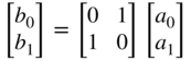
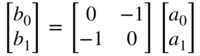
Another important element of wave digital filters is the adaptor. Adaptors are used to connect wave digital filter elements with each other. This can be done in a series or a parallel connection. In a two‐port parallel connection, the voltage and current relations can be easily obtained with
Inserting again the definition of the wave variables, we can construct an unadapted wave equation for a two‐port parallel adaptor
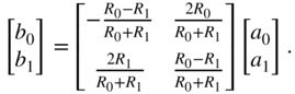
Choosing ![]() for both port resistances, an adapted form can be found with
for both port resistances, an adapted form can be found with
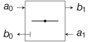
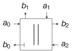
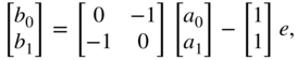
The wave equation for a two‐port series adaptor can be obtained similarly by using ![]() and
and ![]() as voltage and current relations.
as voltage and current relations.
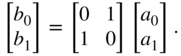
For many applications, adaptors will be needed which have more than two ports. Most commonly used are three‐port adaptors. Furthermore, three‐port adaptors can also be used as building blocks for N‐port adaptors [Wer16]. Consequently, we will only deal with the derivation of three‐port series or parallel adaptors.
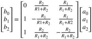
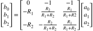
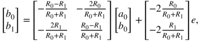
The voltage and current relations of a three‐port parallel adaptor are given by
This can be brought similarly to the two‐port adaptor in an adapted wave equation
with the adapted port resistance ![]() . All adapted wave equations for two‐port as well as for three‐port series and parallel adaptors can be found in Table 10.2.
. All adapted wave equations for two‐port as well as for three‐port series and parallel adaptors can be found in Table 10.2.
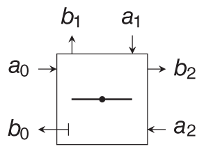
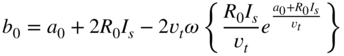
We will conclude this section with a simple example of how to construct a wave digital filter model from a given circuit schematic. An easy nonlinear circuit can be seen in Fig. 10.17. It comprises an asymmetrical second‐order diode clipper. The wave digital filter structure of this circuit can be seen on the left‐hand side of Fig. 10.18. Constructing such a wave digital filter structure underlies certain restrictions and building rules to make the filter realizable. These restrictions can be best understood if we introduce the concept of connection tree structures for wave digital filters. The structure of Fig. 10.18 can be transformed into a tree‐based topology. This structure comprises several elements, namely the root, the leaves, and adaptors. The corresponding connection tree of the wave digital filter can be seen on the right‐hand side of Fig. 10.18. The root of a wave digital filter has no upward facing connections to other elements, an adaptor has one upward facing connection and one or more downward faced ports, and a leaf is an element containing only one upwards facing connection. A non‐adaptable element, such like a voltage source, should always be the root of the connection tree. It is not allowed to be placed as a leaf or adaptor. This can lead to complications if the analog circuit contains more than one non‐adaptable element. For voltage and current sources, this can be solved by combining the source with its adjacent adaptor. The voltage source can be absorbed into a series connection resulting into a two‐port block with the wave equation
where ![]() is the source voltage. This wave equation can be adapted by setting
is the source voltage. This wave equation can be adapted by setting ![]() yielding the adapted wave equation
yielding the adapted wave equation
which can now be used as an adaptor in the connection tree. Going further, the nonlinear elements are also restricting the construction of the wave digital filter. Note that we restricted ourselves in this example to a circuit with only one nonlinear element. The reason for this is that a nonlinear element should always be placed at the root of the wave digital filter. Constructing a filter with more nonlinear elements runs into several problems, whose solutions are a major research area in wave digital filter design. One approach of dealing with multiple nonlinear or non‐adaptable elements is the use of so‐called ![]() ‐type adaptors, which have successfully been implemented to model these kinds of circuits [Wer16]. For the sake of simplicity, we will stick with our simple example in Fig. 10.17. One major advantage of using binary connection trees, like that from Fig. 10.18, is that there is no possibility the graph can have a delay free loop. This property directly assures realizable wave digital filter structures. From the tree structure in Fig. 10.18, a realizable signal flow graph can be derived, which can finally be used to compute the output signal of the wave digital filter.
‐type adaptors, which have successfully been implemented to model these kinds of circuits [Wer16]. For the sake of simplicity, we will stick with our simple example in Fig. 10.17. One major advantage of using binary connection trees, like that from Fig. 10.18, is that there is no possibility the graph can have a delay free loop. This property directly assures realizable wave digital filter structures. From the tree structure in Fig. 10.18, a realizable signal flow graph can be derived, which can finally be used to compute the output signal of the wave digital filter.
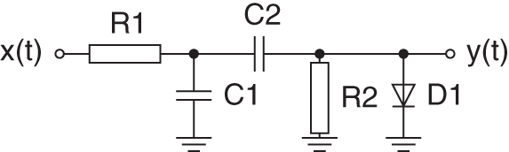
Figure 10.17 Second‐order diode clipper.
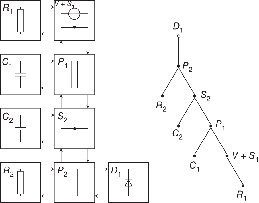
Figure 10.18 Wave digital filter structure of second‐order diode clipper with corresponding connection tree.
10.5.2 State‐space Approaches
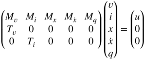
One of the most used approaches in the domain of virtual analog modeling is to derive a nonlinear state‐space model from any given circuit schematic. This can be done very systematically by using, for example, the nodal DK method proposed by David Yeh in [Yeh10]. The resulting nonlinear state‐space model has the form
with ![]() as input vector,
as input vector, ![]() as output vector, and
as output vector, and ![]() and
and ![]() as the voltage over and current through the nonlinear circuit elements. The matrices
as the voltage over and current through the nonlinear circuit elements. The matrices ![]() ,
, ![]() ,
, ![]() ,
, ![]() ,
, ![]() ,
, ![]() ,
, ![]() ,
, ![]() ,
, ![]() describe the dynamics of the system and
describe the dynamics of the system and ![]() is a nonlinear function containing all voltage–current relations of the nonlinear elements. In comparison to the nodal‐DK method, we will derive the state‐space model with an approach introduced in [Hol15]. We will start with the description of individual circuit elements. Any circuit element will be described with the equation
is a nonlinear function containing all voltage–current relations of the nonlinear elements. In comparison to the nodal‐DK method, we will derive the state‐space model with an approach introduced in [Hol15]. We will start with the description of individual circuit elements. Any circuit element will be described with the equation
where ![]() ,
, ![]() are the port voltages and currents,
are the port voltages and currents, ![]() ,
, ![]() are the element's state and state derivative vectors, respectively,
are the element's state and state derivative vectors, respectively, ![]() is the auxiliary vector,
is the auxiliary vector, ![]() the source vector, and
the source vector, and ![]() the element's nonlinear voltage–current relationship. The coefficient matrices of common circuit elements are given in Table 10.3.
the element's nonlinear voltage–current relationship. The coefficient matrices of common circuit elements are given in Table 10.3.
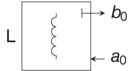
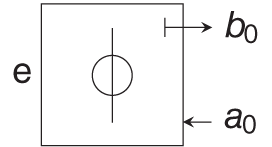
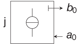
Table 10.3 Coefficient matrices and nonlinear functions of common circuit elements
| Element | |||||||
|---|---|---|---|---|---|---|---|
| Voltage source | |||||||
| Current source | |||||||
| Resistor | |||||||
| Capacitor |  |  |  | ||||
| Inductor |  |  | |||||
| Diode |  |
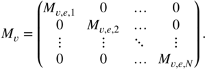
A description of the whole circuit can be now achieved by combining all individual coefficient matrices, nonlinear functions as well as voltage, current, state, state derivative, and source vectors into one system. The vectors are simply stacked like ![]() . The coefficient matrices are combined into one block diagonal matrix with the form
. The coefficient matrices are combined into one block diagonal matrix with the form
The nonlinear functions are collected in the vector
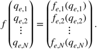
Going further, all constraints introduced by the circuit's elements can be described by
Applying now Kirchhoff's voltage and current laws, the circuit topology can be incorporated with the additional equations ![]() and
and ![]() , where the matrices
, where the matrices ![]() and
and ![]() are derived using standard network analysis techniques. This leads to the nonlinear differential equation system:
are derived using standard network analysis techniques. This leads to the nonlinear differential equation system:
From this point, it is possible to derive a continuous‐time state‐space model, and with subsequent discretization, a discrete‐time model. However, the equation system can also be directly discretized. For that, we decide to use the trapezoidal integration rule for time discretization:
where ![]() is the sampling interval,
is the sampling interval, ![]() the discrete approximation of the state at time
the discrete approximation of the state at time ![]() , and
, and ![]() the exact solution for
the exact solution for ![]() . With the introduction of canonical states,
. With the introduction of canonical states,
we can make use of the substitutions
and the definitions ![]() and
and ![]() to construct a discrete‐time system of the form
to construct a discrete‐time system of the form
where ![]() ,
, ![]() ,
, ![]() , and
, and ![]() are the discrete‐time values at time
are the discrete‐time values at time ![]() . This discrete‐time equation system cannot be solved uniquely; however, a general solution can be obtained with
. This discrete‐time equation system cannot be solved uniquely; however, a general solution can be obtained with
Here, ![]() is an arbitrary vector depending on the chosen solution with as many entries as
is an arbitrary vector depending on the chosen solution with as many entries as ![]() . Finally, we can extract from
. Finally, we can extract from ![]() and
and ![]() only the quantities of interest resulting into a nonlinear state‐space system like in Eqs. (10.47a) to (10.47d):
only the quantities of interest resulting into a nonlinear state‐space system like in Eqs. (10.47a) to (10.47d):
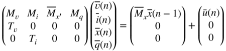
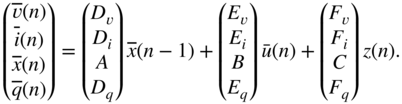
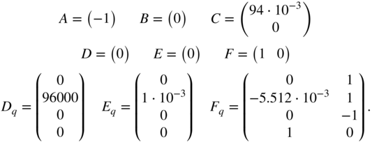
We will demonstrate this approach using again the example from the clipping circuit in Fig. 10.3. By ordering the circuit elements as voltage source, resistor, capacitor, first diode, and second diode, the following coefficient matrices can be found:
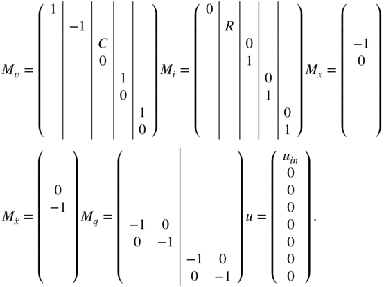
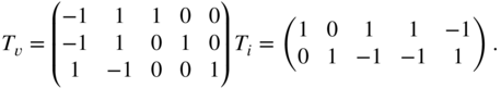
The matrices ![]() and
and ![]() can be constructed using
can be constructed using ![]() and
and ![]() yielding
yielding
After time discretization with a sampling rate of ![]() kHz, we can derive
kHz, we can derive

In the next step, the equation system from Eq. (10.56a) needs to be solved. The general solution of a system of the form ![]() , which has no unique solution, can be constructed by using the nullspace
, which has no unique solution, can be constructed by using the nullspace ![]() of
of ![]() in conjunction with one particular solution
in conjunction with one particular solution ![]() ,
,
where ![]() is an arbitrary vector. From this general solution, we can directly obtain the system matrices
is an arbitrary vector. From this general solution, we can directly obtain the system matrices ![]() ,
, ![]() ,
, ![]() ,
, ![]() ,
, ![]() ,
, ![]() . The matrices
. The matrices ![]() ,
, ![]() , and
, and ![]() can be extracted from
can be extracted from ![]() ,
, ![]() , and
, and ![]() , i.e. we can take the third row of the matrices, which corresponds to the voltage over the capacitor. The resulting matrices yield
, i.e. we can take the third row of the matrices, which corresponds to the voltage over the capacitor. The resulting matrices yield
The output of the nonlinear state‐space system can now be computed by finding a suitable ![]() , which is consistent with (Eqs. 10.58c) and (10.58d). This vector can then be used to solve the linear part of the system comprising (Eqs. 10.58a) and (10.58b). Note that the coefficient matrices might also have different values, owing to the non‐uniqueness of the nonlinear equation system from Eq. (10.56a). Consequently, the coefficient matrices depend on the chosen particular solution and the nullspace.
, which is consistent with (Eqs. 10.58c) and (10.58d). This vector can then be used to solve the linear part of the system comprising (Eqs. 10.58a) and (10.58b). Note that the coefficient matrices might also have different values, owing to the non‐uniqueness of the nonlinear equation system from Eq. (10.56a). Consequently, the coefficient matrices depend on the chosen particular solution and the nullspace.
10.6 Exercises
1. Fundamentals
- What can be said about the output of a memoryless nonlinear system excited with a periodic input?
- Let
 be a static nonlinear mapping excited with
  . Compute the Fourier coefficients of the resulting output
  . What can be said about the THD?
2. Overdrive, Distortion, Clipping
- Derive the nonlinear differential equation for the first‐order diode clipper assuming identical diodes. Hint:
 ,
,  .
.
- What is the difference between soft‐ and hard clipping nonlinearities? How can they be used to create a distortion or overdrive effect?
3. Nonlinear Filters
- How can we extend a linear filter design to give it a more natural sound?
- What is the difference to linear filters regarding the stability?
4. Aliasing and its Mitigation
- Assume a nonlinear system introducing harmonics rolling off with frequency by approximately
 . When operated at a sampling rate of 44.1 kHz, the aliasing distortion is deemed too high. By what factor, approximately, is the aliasing distortion present below 22.05 kHz reduced when doubling the sampling rate?
 - Apply antiderivative antialiasing to the memoryless systems described by the mapping functions of (Eqs. 10.8) and (10.9).
5. Virtual Analog Modeling
- Give an overview of the three main modeling approaches.
- How is a circuit element modeled in the wave domain? State the connection between the wave and Kirchhoff domains.
References
- [Bil17a] S. Bilbao, F. Esqueda, J.D. Parker, and V. Välimäki: Antiderivative antialiasing for memoryless nonlinearities. IEEE Signal Processing Letters, 24(7):1049–1053, 2017.
- [Bil17b] S. Bilbao, F. Esqueda, and V. Välimäki: Antiderivative antialiasing, lagrange interpolation and spectral flatness. In 2017 IEEE Workshop on Applications of Signal Processing to Audio and Acoustics (WASPAA), pages 141–145, New Paltz, NY, USA, Oct 2017.
- [Che04] G. Chen: Stability of nonlinear systems. Encyclopedia of RF and Microwave Engineering, pp 4881–4896, 2004.
- [Cho20] J. Chowdbury: Stable structures for nonlinear biquad filters. In Proceedings of the 23rd International Conference on Digital Audio Effects (DAFx‐20), pages 94–100, Vienna, Austria, 2020.
- [Eic16] F. Eichas and U. Zölzer: Virtual analog modeling of guitar amplifiers with Wiener‐Hammerstein models. In 44th Annual Convention on Acoustics, Munich, Germany, 2018.
- [Esq15] F. Esqueda, V. Välimäki, and S. Bilbao: Aliasing reduction in soft‐clipping algorithms. In Proc. 23rd European Signal Process. Conf. (EUSIPCO), pages 2059–2063, Nice, France, 2015.
- [Esq16a] F. Esqueda, V. Välimäki, and S. Bilbao: Antialiased soft clipping using an integrated bandlimited ramp. In Proceedings of the 24th European Signal Processing Conference (EUSIPCO), pages 1043–1047, Budapest, Hungary, 2016.
- [Esq16b] F. Esqueda, S. Bilbao, and V. Välimäki: Aliasing reduction in clipped signals. IEEE Transactions on Signal Processing, 64(20):5255–5267, 2016.
- [Mul17] R. Muller and Thomas Helie: Trajectory anti‐aliasing on guaranteed‐passive simulation of nonlinear physical systems. In Proceedings of the 20th International Conference on Digital Audio Effects (DAFx‐17), pages 87–94, Edinburgh, UK, 2017.
- [Par16] J.D. Parker, V. Zavalishin, and E. Le Bivic: Reducing the aliasing of nonlinear waveshaping using continuous‐time convolution. In Proceedings of the 19th International Conference on Digital Audio Effects (DAFx‐16), pages 137–144, Brno, Czech Republic, 2016.
- [Par19] J.D. Parker, F. Esqueda, and A. Bergner: Modelling of nonlinear state‐space systems using a deep neural network. In Proceedings of the 22nd International Conference on Digital Audio Effects (DAFx‐ 19), Birmingham, UK, 2019.
- [Fet86] A. Fettweis: Wave digital filters: Theory and practice. In Proceedings of the IEEE, volume 74, 1986.
- [Fra13]Fractal Audio Systems: Multipoint iterative matching and impedance correction technology, 2013.
- [Hol15] M. Holters and U. Zölzer: A generalized method for the derivation of non‐linear state‐space models from circuit schematics. In Proceedings of the 23rd European Signal Processing Conference (EUSIPCO), Nice, France, 2015.
- [Hol20] M. Holters: Antiderivative antialiasing for stateful systems. Applied Sciences, 10(1), 2020.
- [Kem08] C. Kemper: Musical instrument with acoustic transducer. “https://www.google.com/patents/US20080134867”, 2008.
- [Roa79] C. Roads: A tutorial on Non‐Linear Distortion or Waveshaping Synthesis. Computer Music Journal, Vol. 3, No. 2, pp. 29–34, 1979.
- [Ros92] D. Rossum: Making digital filters sound “analog”. ICMC, pp 30–33, 1980.
- [Sche80] M. Schetzen: The Volterra and Wiener Theories of Nonlinear Systems. Robert Krieger Publishing, 1980.
- [Wer16] K. J. Werner: Virtual Analog Modeling Of Audio Circuits Using Wave Digital Filters. PhD thesis, 2016.
- [Wri19] A Wright, E. Damskägg, and V. Välimäki: Real‐time black‐box mod‐ elling with recurrent neural networks. In Proceedings of the 22nd International Conference on Digital Audio Effects (DAFx‐19), Birmingham, UK, 2019.
- [Yeh10] D.T. Yeh, J.S. Abel, and J.O. Smith: Automated physical modeling of nonlinear audio circuits for realtime audio effects part I: Theoretical development. IEEE Trans. Audio, Speech and Language Process., 18(4):728–737, 2010.