2
Baseband Digital Transmission: Problems 16 to 26
2.1. Problem 16 – Entropy and information to signal source coding
We consider the problem of long-distance transmission over low cost electric cable of a compressed information source S from a video signal compression ystem. The compression system used makes sure that the source S delivers words s a a dictionary with only five words: [s1, s2, s3, s4, s5] . The probabilities of issuing symbols are given in Table 2.1.
Table 2.1. Probability of emission of source S
| s | s1 | s2 | s3 | s4 | s5 |
| Pr(s) | 0.11 | 0.19 | 0.40 | 0.21 | 0.09 |
The symbols are delivered by the source with a rate of 13.5 × 10⁶ symbols per second.
- 1) Determine the entropy H (S) of the source S. Deduce the entropy rate per second. What would be the efficiency η1 of a fixed-length code C1, its length L1, and the bitrate per second, denoted D1?
- 2) Construct the Huffman code C2 generating the codeword Si associated with each of the symbols si
NOTE.– In the design of the code C2, the coding suffix associated with the element of lower probability will be systematically set to 1.
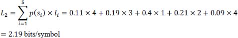
Deduce the average length L2 of the codeword C2, its efficiency η2 and the bitrate per second D2
- 3) It is considered here that the source S delivers the following time sequence SS of symbols s:
Deduce the corresponding sequence SB of bits obtained at the output of the Huffman coding C2 . SB is of the form { ⋯⋯ bk–1, bk, bk+1 ⋯⋯}. What do you observe?
- 4) The transmitter constructs a baseband signal supporting the transmitted information bits.
- a) It first uses a bipolar encoder (called CODBip) of RZ type, with amplitude V and duration Tb. Draw a graph of the signal portion associated with SB transmitted by this CODBip encoder. What are the problems encountered in reception?
NOTE.– Both here and also in question b), we will consider, at the start of the sequence, that the parity flip-flop of the number of “1” is equal to 1.
- b) It then uses an encoder (called CODHDB) of HDB-2 type. Draw a graph of the signal portion associated with SB transmitted by this CODHDB encoder. Are some problems solved now and why?
- c) What is the approximate bandwidth of the signal emitted by the bipolar or HDB-2 code to encode the S source? (We can rely on the properties of the power spectral density Γ (f) of the signal transmitted). To transmit this source of information on this type of cable, is there a good fit?
- a) It first uses a bipolar encoder (called CODBip) of RZ type, with amplitude V and duration Tb. Draw a graph of the signal portion associated with SB transmitted by this CODBip encoder. What are the problems encountered in reception?
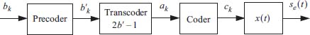
- 5) We want to reduce the bandwidth of the transmitted signal. Thus, it is desired to use an information-to-signal coder of partial response linear encoder type. This encoder will be very simple, of the form 1 – D2 (here D is the delay operator of Tb, time slice allocated to the transmission of a binary symbol). The signal x (t) which carries the symbols ck is of NRZ type, amplitude V/2 and duration Tb.
The following SBB binary sequence will be used for the rest of this problem:

- a) This type of encoder needs to be preceded by an appropriate precoder. Why?
- b) Describe the relationship between the pre-encoder output (giving the symbols
 ) and its input bk.
 - c) Describe the relationship between the encoder output (producing the symbols ck) and its input ak
- d) Represent graphically, the signal portion associated with SBB transmitted by this whole partial response coder (for a pulse amplitude modulation of duration Tb). It will be necessary to first determine the sequence obtained at the output of the precoder (it will be assumed that the two symbols
 not known at the beginning of the sequence are zero).
 - e) What is the approximate bandwidth of the signal emitted by this partial response linear code to encode the source S ? Have we gained any bandwidth reduction?
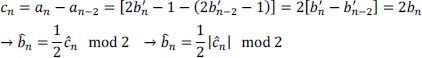
- 6) For this partial response linear code, how does decoding produce the symbols bk from ck? Justify your answer. What happens to the reconstructed binary information
 if a transmission error occurs for one of the symbols ĉk reconstructed on reception?
Solution of problem 16
- 1) Entropy H (S)

Entropy bitrate:
Fixed-length code C1 (length L1): we have five symbols to encode, hence: L1 = 3 bits.
Efficiency:
Bitrate of code C1:
- 2) Huffman code C2.
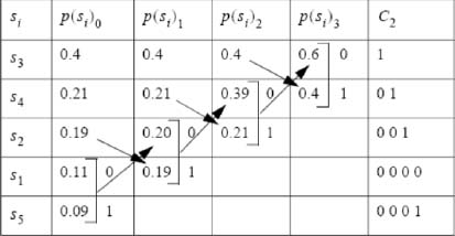
Average length of the codewords:
Efficiency of code C2
Bitrate of code C2:
- 3) Sequence S B of bits obtained at the output of the Huffman coding.
| SS | s2 | s5 | s3 | s4 | s3 | s3 | s2 | s3 | s5 | s4 |
| SB(s) | 011 | 0001 | 1 | 01 | 1 | 1 | 001 | 1 | 0001 | 01 |
More bits are observed at zero than at one and, in addition, we have sequences of three consecutive zeros from time to time.
- 4) Information for baseband signal encoding.
- a) Bipolar CODBip encoder of RZ type (see the graph in Table 2.4). The problems encountered in reception are related to the difficulties of getting a correct clock recovery in some cases, here three consecutive zeros, because the encoder produces no pulse for duration 3T.
- b) CODHDB coder of HDB-2 type: look at the graph in Table 2.4.
Sequences of three consecutive zeros are replaced by sequences of type “ 0 0 V” or “B 0V “ and thus, we can have a maximum duration of 2T without impulse.
- c) The power spectral density of the RZ bipolar code is given by:
The zeros of IRZ (f) occur every 1/Tb, so its bandwidth is 1/Tb. It is substantially the same for the HDB-n code (here HDB-2).
Furthermore, in the vicinity of the frequency f = 0, the power is zero, this code can therefore be used for long-distance cable transmission. However, the presence of long sequences of zeros is detrimental to the clock recovery, therefore we use the code HDB – n.
- 5) Partial response code (PRC).
- a) Yes, it is necessary to use a pre-encoder so that on reception, the decoding is instantaneous (without recursion) and therefore, if a decoding error occurs, it does not propagate recursively.
- b) Pre-encoder output (symbol
 ) as a function of its input bk

- c) Relationship between the encoder output (symbol ck) and its input ak:

- d) Graphical representation of the signal portion associated with SBB transmitted by this whole partial response coder: look at the graph in Table 2.4.
- e) The power spectral density of the partial response code concerned is given by (see Volume 1, Chapter 5):

The zeros of ![]() take place every 1/2Tb, its bandwidth is then approximately 1/2Tb
take place every 1/2Tb, its bandwidth is then approximately 1/2Tb
Thus, there is a reduction of the bandwidth of the transmitted signal by a factor of 2, compared to question 4, because of the introduction of the correlation. In addition, one has no continuous component.
- 6) We have:

hence, an instantaneous decoding (no recursion). Thus:
- – if no decision error on ĉk, then, no decision error on

- – if decision error on ĉk, then decision error on
 only (not on subsequent ones).
- – if no decision error on ĉk, then, no decision error on

Table 2.4. Chronograms of the signals and coded symbols. For a color version of this table, see whw.iste.co.uk/assad/digita/2.zip
2.2 Problem 17 – Calculation of autocorrelation function and power spectral density by probabilistic approach of RZ and NRZ binary on-line codes
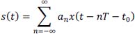
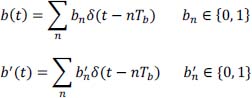
We consider the digital transmission signal defined by:
and:
with:
The symbols an are independent random variables which can take only the values 0 and 1 with a probability equal to 1/2 and t0 is random, of uniform law on the time interval [0, T[.
NOTE.– In this problem, we consider that the instant t belongs to the time interval [t0, t0 + T[. Without any loss of generalities, we will assign the index n to this ight. interval where the time t is a priori.
Calculate the autocorrelation function Rs (τ) and the power spectral density Γs (f) of s (t) and carry out the two particular cases:

Figure 2.2. Examples of binary RZ and NRZ codes. For a color version of this figure, see www.iste.co.uklassad/digital2.zip
Solutionof problem 17
Let us make the following form of the signal s (t) (with θ < T/2 on Figure 2.3).

Figure 2.3. Example of signal s(t) waveform with θ < T/2
Such a signal can be represented by:
With the deterministic function (pulse):
and:
since t0 is uniform on time interval [0, T[, then s (t) is a second-order stationary random signal.
Moreover, the autocorrelation function Rs (τ) is an even function: Rs (–τ) = Rs (τ) and thus the calculation can be done with suitability with τ ≥ 0 or τ ≤ 0.
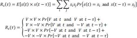
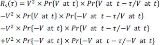
The autocorrelation function Rs (τ) is written:

hence:
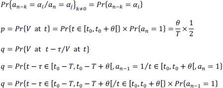
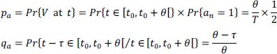
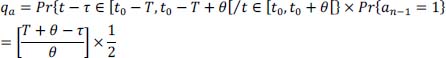
Moreover, using the theorem of compound probability, Rs(τ) is also written:
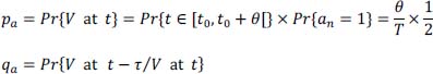
To calculate Rs(τ), it is sufficient to calculate Pr{V at t} and Pr{V at t–τ/V at t}
A. First case, where 0 < θ ≤ T/2
There are three situations to consider.
- – First situation: 0 ≤ τ ≤ θ
The only possibility is that t and t – τ belong to the same first part of time slice (hatched region).

Let:
and:
or, since an = 1
that is to say:
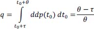
Or:
with random t0, of a posteriori law uniform over a measurement interval θ therefore with probability density (ddp(t0)) equal to 1/θ
Hence:
So finally:
NOTE.– In general, if a priori t belongs to a time interval, of measurement T (t0 is random, of uniform law on time interval [0, T[), we know a posteriori that t belongs to a first part of the time interval, of measure θ. It is therefore this posterior uniform law that is used in time conditional probabilities.
- – Second situation: θ < τ ≤ T
The only possibility is that s(t) and s(t – τ) come from two first parts of adjacent time slots, hence independence between the variables a considered.
In general, we will always have:
and:
turns into:
Or:
Which depends on the value of τ with respect to θ and T
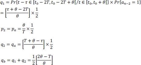
Two situations can occur (see graph in Figure 2.5).
We know that if a real random variable follows a uniform law over a given interval [c, d] , then its probability density is equal to 1/Mes [c, d] and that:
and if Mes[c, d] = 0, then the probability density will be zero because we are faced here with a continuous random variable
if: θ < τ ≤ T, then:

So if θ < τ ≤ T – θ, the measure of the interval is zero, thus q = 0
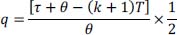
Otherwise, if T – θ < τ ≤ T, then the measure of the interval is given by:
τ + θ – T, and:
So if:
and if:
- – Third situation: τ > T
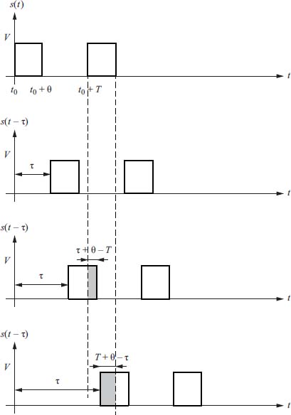
Figure 2.5. Second and third situations
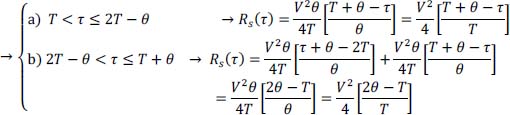
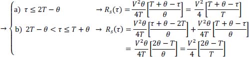
In summary, for 0 < θ ≤ T/2, if:
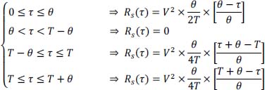
For values τ > T + θ, we see that the intervals intervening in the conditional probability relating to instants (t – τ) and t are different and therefore n – k < n. This implies that conditional probability Pr{an–k/an}k≠0 = Pr{an–k}, and that the probability relating (t – τ) conditionally to t will evolve periodically, from T to T strictly as we have just described it. More precisely, we have:
- – for: θ + kT ≤ τ < (k + 1) T – θ, then q = 0
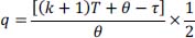
- – for: (k + 1) T – θ ≤ τ < (k + 1) T, then:
- – for:(k+1) T leq τ < (k+1) T+ θ , then
- – for: (k + 1) T + θ ≤ τ < (k + 2) T – θ, then q = 0
It is therefore a periodic function of period T
Note that the autocorrelation function breaks down into a sum of two functions:
with R1 (τ) , a non-periodic function, and R2 (τ), a periodic function of period T
Calculation of the power spectral density Γs(f)
Calculation of the power spectral density Γ1(f)
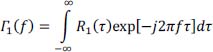

Figure 2.6. Autocorrelation function Rs (τ) and its decomposition
R1 (τ) is an even symmetric function, hence:
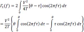
but:

and:
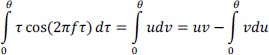
Integration by part, with:
u = τ and v = cos(2πfτ)dτ
hence:
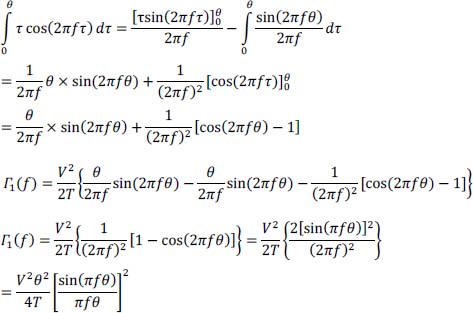
which is a classic result. Indeed, recall that if:

then:
Γ1 (f) has a continuous spectrum.
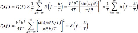
Calculation of Γ2 (f)
The basic form of R2 (τ) is identical to that of R1 (τ) and in addition, it is periodic with period T, then:
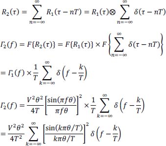
It is a discrete spectrum, the discrete spectral components being spaced 1/T apart from each other.
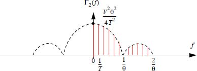
Figure 2.8. Discrete spectral components of the power spectral density I2 (f) For a color version of this figure, see www.iste.co.uk/assad/digita/2.zip
Special case where θ = T/2: binary RZ code.
In this case, we then have:
and:

The continuous component is such that:
Γ2(0) = [continuous component]2 × δ(f)
One has:
Thus, the continuous component is then equal to V/4
The function sin(kπ/2) is non zero for odd integer k, so by setting k = 2n + 1 the expression of Γ2 (f) is then written:
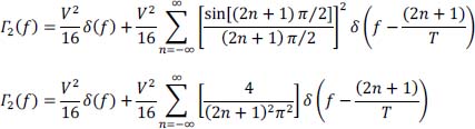
This is also written:

Γ2 (f) has discrete components at odd frequencies and in particular at the frequency f = 1/T which makes it possible to recover the clock.
B. Second case, the one where T/2 < θ ≤ T
There are also three situations to consider.
- – First situation: 0 < τ ≤ θ
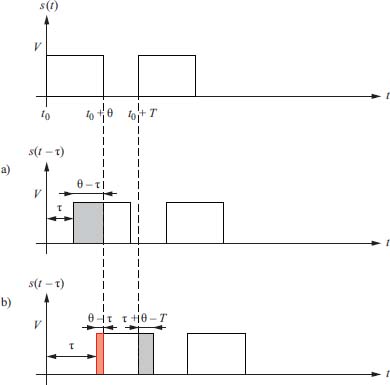
Figure 2.9. First situation: 0 < τ ≤ θ (with T/2 < θ ≤ T). For a color version of this figure, see www.iste.co.uk/assad/digita/2.zip
Calculation of p and q. There are two cases:
- a) τ + θ ≤ T → t and t – τ∈ the same first part of time slice:
- b) τ + θ >T, there are two possibilities:
First possibility: t and t – τ do not belong to the same first part of the time slice, but to the first parts of adjacent time slices:

Or:
Second possibility: t and t – τ belong to the same first part of the time slice, hence:
NOTE.– Both hypotheses a) and b) exclude each other.
Thus, for:

Note that in the case a), the expression of Rs (τ) is also valid throughout the time interval τ ∈ [0, θ]
- – Second situation: θ ≤ τ < T
The only possibility is that s (t) = V and s (t – τ) = V come from the first two parts of adjacent time slices.

Let’s set:
and:

hence:
- – Third situation: T ≤ τ < T + θ.
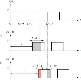
Figure 2.11. Third situation: T ≤ τ < T + θ . For a color version of this figure, see www.iste.co.uk/assad/digita/2.zjp
Calculation of p and q. There are two cases:
- a) T < τ ≤ 2T – θ → t and t – τ ∈ to the first two parts of adjacent time slices:
Following the same approach as in the previous situation, we obtain:
- b) 2T – θ < τ < T + θ , there are two possibilities:

NOTE.– Both hypotheses a) and b) exclude each other.
Thus, for T ≤ τ < T + θ:
Note that in case a), the expression of Rs (τ) is also valid throughout the time interval [T ≤ τ ≤ T + θ]
In summary, for T/2 < θ ≤ T:
- – for 0 < τ ≤ θ

- – for θ ≤ τ < T:
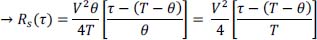
- – for T ≤ τ ≤ T+ θ:
As in the case 0 < θ ≤ T/2, the probability relating to (t – τ) conditionally at t will evolve periodically from T to T, strictly as we have just described it above.
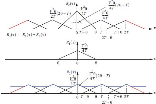
Figure 2.12. Autocorrelation function Rs (τ) and its decomposition. For a color version of this figure, see whw.iste.co.uk/assad/digita/2.zip
In the same way as for 0 < θ ≤ T/2, the autocorrelation function breaks down into a sum of two functions:
with R1(τ) , a non-periodic function, and R2(τ), a periodic function, of period T. In addition, we note that the expression of R1(τ) and R2(τ) are the same as previously (case 0 < θ ≤ T/2).
Calculation of the power spectral density, case where: T/2 < θ ≤ T
The power spectral density of the signal s (t) can be broken down into the sum of two functions:
with:
This is a continuous spectrum.
And:
This is a discrete spectrum.
Special case: θ = T (NRZ code)
In this case, we obtain:

So:
Thus, finally we get:
Notice that for θ = T (NRZ code), the signal does not have a discrete spectrum component at 1/T (Γ2 (f) is zero for the other values of k ≠ 0). Therefore, clock recovery is not easy with NRZ code.
NOTE.– One could easily generalize the problem to the situation where the symbols of information to be transmitted are not equiprobable: Pr {a = 0} = λ and: Pr{a = 1} =1 – λ
2.3. Problem 18 – Calculation of the autocorrelation function and the power spectral density by probabilistic approach of the bipolar RZ code
The bipolar RZ code is a three-level code such as:
and:
The binary random variables are assumed to be equiprobable:
We consider the digital transmission signal defined by:
The signal is a second-order stationary random signal assuming that the time of origin t0 is random and uniformly distributed over the time interval [0, T[.
NOTE.– In this problem, we consider that the instant t belongs to the time interval [t0, t0 + T[. Without any loss of generalities, we will assign the index n to this ight. interval where the time t is a priori.
Moreover, as for problem 17, one could immediately generalize to the situation where the information source does not generate equiprobable b symbols.
However, we preferred not to complicate the problem. For those who wish to do so, after having analyzed the situation in the equiprobable case, it will be easy to generalize the results to a situation with a non-equiprobable source.
Calculate the autocorrelation function Rs(τ) and the power spectral density Γs(f) of the signal s(t)
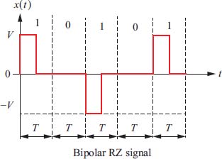
Figure 2.13. Example of a bipolar RZ signal waveform. For a color version of this figure, see www.iste.co.uklassad/digita/2.zjp
Solutionof problem 18
The signal s (t) can be represented by:
where:
is a deterministic function, and:
The autocorrelation Rs(τ) is written:
Using the theorem of compound probabilities, Rs(τ) is written as:
Calculation of the simple probabilities Pr{V at t} and Pr{–V at t}
since there is independence between t0 and the symbols of information, we have:
Likewise:
and:
Besides:
And yet:
as we have two mutually exclusive hypotheses, hence:
thus:
and:
Let’s now calculate the other probabilities, representing four mutually exclusive hypotheses. Note that for reasons of symmetry, we have:
and:
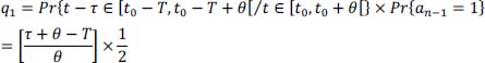
- – First case: 0 ≤ τ ≤ T/2
- 1) Let:
The only possibility is that t and t – τ belong to the same first half of the time slice:
We have:

Figure 2.14. First case: 0 < τ < T/2 and a positive impulsion at t. For a color version of this figure, see www.iste.co.uk/assad/digital2.zip
therefore:
- 2) Let:
So, we have: q2 = 0
So, we have also:
and:
- – Second case: T/2 < τ ≤ T
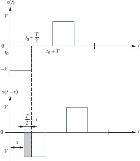
Figure 2.15. First case: 0 ≤ τ ≤ T/2 and negative impulse at t . For a color version of this figure, see www.iste.co.uk/assad/digita/2.zip

Figure 2.16. Second case: T/2 < τ ≤ T . For a color version of this figure, see whw.iste.co.uk/assad/digita/2.zip.
The only possibility is that t and t – τ∈ first halves of adjacent time slices.
Since two successive bits to 1 are issued in alternating polarity, then:

yet:
(due to the independence between binary information symbols).
And on the other hand:

hence:
and, by symmetry, we have:
- – Third case: T < τ ≤ T + T/2
The only possibility is that t and t – τ belong to the first two halves of adjacent time slices.
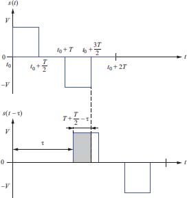
Figure 2.17. Third case: T < τ ≤ T + T/2 . For a color version of this figure, see www.iste.co.uklassad/digita/2.zip
Since two successive bits at “1” are issued in alternating polarity, then as explained previously:
hence:
We have:
and, on the other hand:

hence:
and, by symmetry, we have:
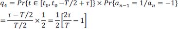
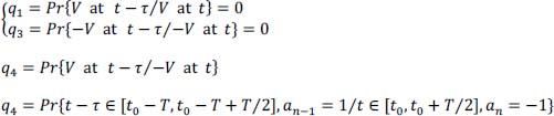
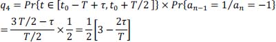
- – Fourth case: 3T/2 < τ ≤ 2T.
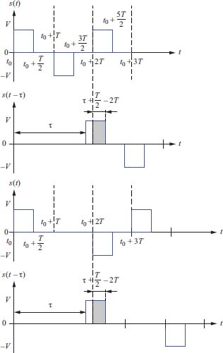
Figure 2.18. Fourth case: 3T/2 < τ ≤ 2T . For a color version of this figure, see www.iste.co.uklassad/digital2.zjp
The only possibility is that (t – τ) and t belong to two first time slices separated by a time slot of intermediate duration T:
Moreover, since we have the conditional event: {V at (t – τ)/V at t} , we must also have in the intermediate time slot a negative impulse, and therefore a symbol an–1 = –1
Therefore:
Because of the statistical independence between the pairs of instants considered and the values of the symbols considered, we have:
The first conditional probability on the instants gives:

The second conditional probability on the symbols gives (because of the independence between the symbols):
and due to the independence between the symbols b:
hence:
and, by symmetry, we have: q3 = q1 and therefore:
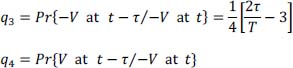
As before, the only possibility is that t – τ and t each belong to two first time slices separated by a time slice of intermediate duration T but, unlike in the previous case, in the intermediate time slice, it must not have transmitted a pulse, therefore a symbol: an–1 = 0 . The conditional probability for the instants remains the same. It is the same for conditional probabilities on symbols a. As a result, we have:
and therefore:
And by symmetry, we also have q2 = q4 and therefore:
Consequently, we finally get:
Actually, we show that for:
Indeed, let’s take for example the case: 2T ≤ τ < 5T/2.
From the study of the previous case, we see that:

Likewise:
So in the general case where: kT < τ ≤ (k + 1/2)T and k ≥ 2, we have: Rs(τ) = 0
Indeed, (for clarity, see the case: 3T/2 < τ ≤ 2T), we have:
That is:
Because of the independence between t0 and the information symbols a, we therefore have:
or:
with:
and:
This last conditional probability implies implicitly the fact that between n – k and n, we have an odd number of bits bn–k′ at 1 (0 < k′ < k)
Thus:
Because of the independence between the symbols, then one obtains successively:
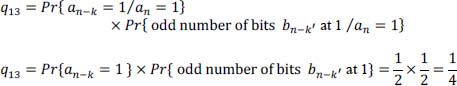
because it is obvious that on a given bit length k, the probability of having an even number of bits at 1 is identical to having an odd number. Indeed, for each given configuration of k – 1 bits, there are two configurations of the additional bit (whatever its position in the k bits): one with 0, the other with 1.
So we have: ![]() .
.
By symmetry, we also have:
In addition, we also have:
i.e.: q4 = q11 × q42
with:
For the same reasons as previously with the calculation of q13, it is easy to show that:
and with the independence of the information symbols:
By symmetry, we also have:
because:
Thus, we obtain:
In summary:
for:
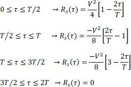
The autocorrelation function Rs (τ) of the bipolar RZ code represented in the Figure 2.19 a shows that it can be decomposed into the sum of two functions R1 (τ) and R2 (τ) represented in the Figure 2.19b
The power spectral density Γs (f) of the bipolar code is therefore given by:
with:
–Γ1 (f) , power spectral density of the signal whose autocorrelation function is R1 (τ) of triangular shape. It is given by:
–Γ2 (f) , power spectral density of the signal whose autocorrelation function is R2 (τ) of trapezoidal shape. And if g (τ) has a trapezoidal form (see Figure 2.20)

Figure 2.19. (a) Autocorrelation function of the bipolar RZ code and (b) its decomposition into the sum of two functions. For a color version of this figure, see www.iste.co.uk/assad/digital2.zip

Figure 2.20. Trapezoidal function. For a color version of this figure, see www.iste.co.uk/assad/digita/2.zip
It is obtained by convolution between two even rectangular functions that do not have the same support in general. Hence:
Let’s apply this to R2 (τ) , with:
Thus, we have successively:

Hence:

Finally, it gives:

Figure 2.21. Power spectral density of the bipolar RZ code. For a color version of this figure, see www.iste.co.uklassad/digita/2.zip
Properties of Γs (f)
– no continuous component;
– no energy at frequency f = 1/T, however a double alternation rectification of the bipolar RZ code gives a RZ code which has a discrete component at frequency f = 1/T in its power spectral density and therefore, a rather easy clock recovery;
– more than 90% of the energy is located in the physical frequency band [0, 1/T]
2.4. Problem 19 - Transmission using a partial response linear coding
We consider the transmission system using the partial response linear coding of Figure 2.22
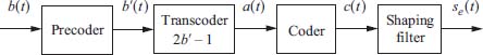
Figure 2.22. Transmission system with partial response linear encoder
- 1) Explain in no more than two sentences the interest of the use of a partial response linear encoder for the baseband transmission of independent binary symbols bn
- 2) Why is it advantageous to use a precoder associated with the partial response linear coder at the transmitter side? Is this precoder necessary for reception? Why?
A partial response linear encoder of the form 1 – D2 where D is the delay operator of Tb (time slice dedicated to the transmission of symbol cn) is used.
- 3) Give the construction rule of cn from an. Deduce the associated precoder: you will give the construction rule of
 as a function of bn.
We consider the following 21 -bit sequence {bn} (time running from left to right:

- 4) Determine:
- –the associated time sequence
 at the output of the pre-coder (the latter is considered initialized to zero);
 - –the time sequence {an} at the output of the transcoder;
- –the time sequence {cn} at the output of the encoder.
- –the associated time sequence
- 5) Give the decoding relationship providing the
 as a function of ĉn.
Let x (t) be the following deterministic pulse (return to zero code, RZ):

And the signal transmitted (without pre-filtering) is se (t).
- 6) How is it related to the sequence {cn} ? Represent on a time diagram the signal se (t) transmitted, for the sequence of binary information {bn} in question 4 . In this example, does the signal transmitted have a continuous component? On statistical average, does this signal have a continuous component?
- 7) If the bn are equiprobable and independent, determine the probabilities of achievement of each element of the alphabet of symbol cn.
- 8) Determine the power spectral density function Γse (f).
- 9) We now consider the following 21 -bit time sequence {bn} (time running from left to right):
Use the HDB-3 coding scheme (high density bipolar pulse code of order 3) to represent the signal sHDB–3 (t) carrying the information and represent it on a time diagram.
Solution of problem 19
- 1) It makes a spectrum shaping. This is performed by the introduction of a certain correlation. The effect is a reduction of the frequency bandwidth of the signal transmitted.
- 2) A precoder is associated with the encoder to ensure that the decoding of the symbols bn is instantaneous. The precoder is not necessary in reception because the decoding is instantaneous.
- 3) since we have:
then:
- 4) Time sequence.
Table 2.5. Chronogram of the time sequence and of the transmitted signal. For a color version of this table, see www.iste.co.uk/assad/digital2.zip

- 5) From the previous relation, we have:
- 6) We have:
The chronogram of the signal se (t) is shown in Table 2.5 above (answer to question 4).
In this sequence, we have a continuous component, since there are five +V pulses and three –V pulses. This continuous component has the value:
Value 2 in the denominator comes from the fact that the signal x (t) is of type RZ
On a statistical average: E { se (t) } = 0 . (i.e. no continuous component)
- 7) since {bn} are equiprobable, then:

- 8) The power spectral density Γse (f) is given by:
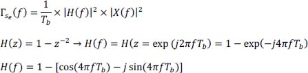
hence:

since:

Furthermore:
hence:
finally, we have:
This code is well suited to long distance cable transmissions because:
- – it has no continuous component, and no power spectral density at very low frequencies;
- – from a practical point of view, most of its power is distributed in the frequency band [0, 1/2Tb].
- 9) High density pulse code: HDB-3 (sHDB-3(t) signal).
Table 2.6. Generation of the HDB - 3 signal and chronogram. For a color version of this table, see www.iste.co.uk/assad/digital2.zip
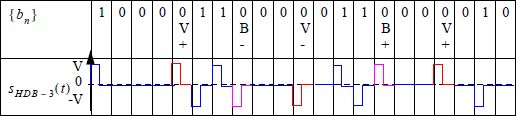
With V: polarity alternation violation bit (bit of violation); B: stuffing bit.
2.5. Problem 20 - Signal information coding and digital transmissions with partial response linear encoder
We consider the problem of long-distance transmission (d > 1Km) over an electrical cable of a source S, of equiprobable binary symbol information, and delivering a binary symbol every Tb seconds. To illustrate this problem, it will be considered that a limited (20-element) length realization of the binary symbol sequence produced by S is:
The amplitude of the modulated pulses is equal to V except for the partial response coding where the amplitude will be V/2.
NOTE.– For a better comparison, time representations of transmitted signals si (t) i = {1, ⋯ , 4} will be drawn on the same sheet, as well as the sequences ![]() , {an} and {cn}.
, {an} and {cn}.
In order to construct the signal s1 (t) carrying the information, a binary return to zero code (RZ code ) is used.
- 1) Represent the signal s1 (t) carrying the sequence {bn } . Is this RZ code of interest for long distance digital transmissions? Justify precisely the reasons for this (you can rely on the properties of the power spectral density Γ1 (f) of s1 (t) to argue).
A bipolar code of the RZ type is now used to construct the signal s2 (t) carrying the information to be transmitted.
- 2) Represent the signal s2 (t) encoding the sequence {bn } . Is this code more interesting than the first one? What are the qualities and defects of long-range transmissions (argue based on the properties of power spectral density Γ2 (f))
We want to use a code with a high density of pulses of type HDB-2.
- 3) Represent the signal s3 (t) carrying the sequence {bn} of information transmitted. What are the characteristics of such a code compared to the RZ bipolar code? What do you conclude about its suitability for long-range transmissions over an electric cable of binary information?
We want to further reduce the bandwidth of the transmitted signal. For this, we use a partial response linear coding as shown in the diagram of Figure 2.24, with:
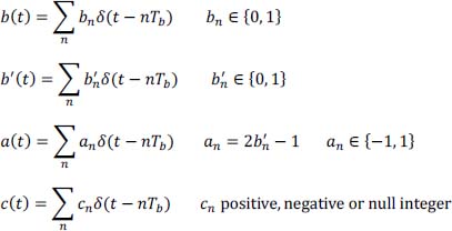

Figure 2.24. Block diagram of the partial response linear coder
The structure of the partial response coder is given in Figure 2.25.
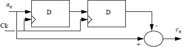
Figure 2.25. Structure of the partial response linear coder (D: D flip-flop synchronized on the binary symbol clock)
- 4) Describe the relationship between the cn output of the encoder and its input an. Why does the encoder have to be preceded by a precoder?
- 5) Describe the relationship connecting the output of the precoder
 to its input bn (the precoder used is obviously that associated with the partial response linear coder
 - 6) For the sequence {bn}, give successively the sequences obtained:
- – at the output of the precoder;
- – at the output of the transcoder;
- – at the output of the linear partial response coder (it will be considered that the
 are zero for the two instants preceding the beginning of the sequence {bn}).
- 7) Represent the signal s4 (t) coding the sequence {bn} obtained at the output of the partial response coder for a RZ shaping signal x (t) of amplitude V/2.
- 8) Determine the power spectral density Γ4 (f) of this partial response linear code. Is it adequate for long distance transmission?
- 9) For this partial response linear code, how does the decoding produce
 from ĉn Justify your answer.
 - 10) What happens to the reconstructed binary information
 if an error (due to transmission) occurs for one of the ĉn symbols reconstructed on reception?
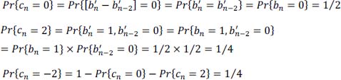
 - 11) Considering that the symbols bn are independent (besides being equiprobable), determine the probabilities of realization of each of the possible values of the symbols cn
Solution of problem 20
Chronograms of the different signals:
Table 2.7. Temporal representations of the different signals. For a color version of this table, see www.iste.co.uklassad/digital2.zip
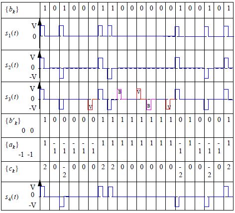
- 1) Look at chronograms of the different signals.
The power spectral density Γ1 (f) of the RZ code is:
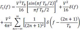
This code is not interesting for transmission over long distance cable because:
- – it has a continuous component equal to V/4 and a high power spectral density at low frequencies;
- – the spectral occupancy of the code is practically 2/Tb, twice that of the NRZ code.
However, the presence of a discrete component at the frequency 1/Tb in the power spectral density facilitates the recovery of the clock rate in reception.
- 2) See the graph of the temporal representations of the different signals in Table 2.7. The power spectral density Γ2 (f) of the bipolar code RZ is:
Benefits of this code:
- – it has no continuous component, and no power spectral density at very low frequencies;
- – its spectral occupancy is only 1/Tb.
Disadvantage of this code: it does not produce pulses to encode a sequence of consecutive 0, therefore the receiver may lose synchronization.
- 3) See the graph of the temporal representations of the different signals in Table 2.7. The HDB code has the same advantages as the bipolar code RZ, but in addition we always have pulses even if a long sequence of 0 is presented. So, it has a good match for the transmission of binary information over long distance cable.
- 4) We have:
The precoding makes it possible to perform in reception (after transmission) an instantaneous decoding.
- 5) We have:

- 6) and 7) See the graph of the temporal representations of the different signals in Table 2.7.
- 8) The power spectral density Γ4 (f) is:
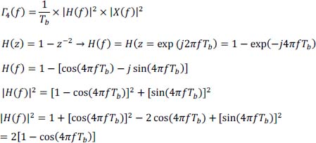
Since:

Furthermore:
hence:
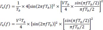
This code is well suited for long distance cable transmission because:
- – it has no continuous component, and no power spectral density at very low frequencies;
- – its spectral occupancy is only 1/2Tb.
- 9) We have:
- 10) If error on ĉn, we have:
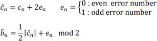
Thus, decision error on bn if en is odd (en = 1) and no decision error on bn if en is even (en = 0).
- 11) We have:
Independence:
For the reasoning that follows, see the graph of the temporal representations of the different signals:
2.6. Problem 21 – Baseband digital transmission system (1)
A baseband digital transmission system of binary information is considered. It transmits coded digital images (with information compression) on a reduced capacity transmission channel (cable). The characteristics of the system in Figure 2.26 will be studied.
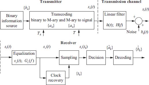
Figure 2.26. Block diagram of the baseband transmission system
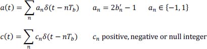
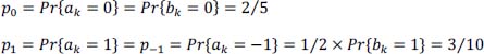
The random sequence {bn} is of a given probability law and bn are assumed to be independent. The transcoding of binary information sequence {bn} into symbol sequence {an} corresponds to the following assignment:
with the following probability law:

The symbols an of information to be transmitted are supplied to the transmitter at a rate of 1/T = 13.5MHz which corresponds to the sampling frequency of the luminance signal in television (standard CCIR 4: 2: 2).
The transmitted signal se (t) is given by:
where x (t) is a rectangular signal of amplitude V and duration:
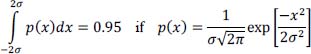
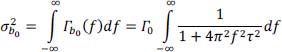
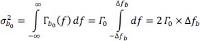
The transmission channel is modeled by a linear filter whose impulse response is denoted by h (t) (the propagation delay is not taken into account) and an additive degradation noise b0 (t) at the output of the channel. The noise b0 (t) is assumed to be a second-order stationary Gaussian random process, independent of the useful signal. It has a zero mean value, a power ,![]() and its power spectral density Γb0 (f) is modeled by a rectangular function of support Δfb (on positive frequency axis) as shown on Figure 2.27.
and its power spectral density Γb0 (f) is modeled by a rectangular function of support Δfb (on positive frequency axis) as shown on Figure 2.27.

Figure 2.27. Power spectral density Γb0 (f) of noise b0 (t)
The equalization of the channel is performed by a linear filtering of the signal received sr (t) : impulse response filter gc (t) , frequency gain Gc (f) such that its support is fully included in the frequency band of the noise b0 (t)
The clock regeneration system is assumed to be flawless, and thus provides the decision system with a sequence of decision instants {tk} with tk = t0 + kT (thereafter, t0 is assumed to be zero).
The decision system uses a given decision threshold μ0 and the decision rule is as follows:

Decoding {ȃk} → {bk} is obvious.
We denote successively:
where ⊗ is the convolution product.
The frequency gain of the equalizer Gc (f) is assumed to be equal to 1 at zero frequency: Gc (0) =1
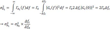
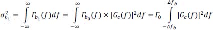
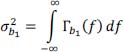
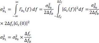
- 1) Determine the noise characteristics b1 (t) at the output of the equalization: the power spectral density Γb1 (f) and the power
 of the noise b1 (t) , as a function of that
  of b0 (t) , its bandwidth Δfb and the energy bandwidth Δfc of the equalization filter.
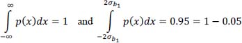
From now on, the equalization filter is assumed such that the amplitude spectrum P (f) of p (t) is constant, equal to VT on the frequency domain
 and equal to zero otherwise.
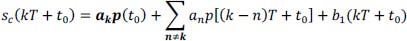
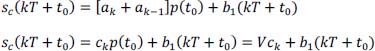
 - 2) Give the expression of the signal sc (tk) (made of the useful signal + intersymbol interference + noise) at the instants of the form: tk = kT.
Subsequently, for sake of simplification, it will be considered that only the two symbols adjacent to a given symbol ak can interfere with it (namely symbols ak-1 and ak+1, and that α = 1/6.
- 3) Calculate the probability pml and the intersymbol interference Iml (tk) for each possible message ml interfering with ak. (For the sake of simplification, take π ≅ 3 in the rest of this problem).
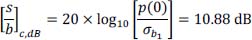
Assuming that at the output of the equalizer the signal-to-noise ratio obtained is:
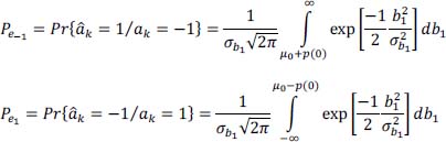
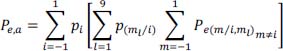
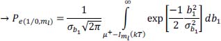
- 4) Give the expressions of the conditional probabilities of error:

- 5) For each possible message ml, calculate these probabilities.
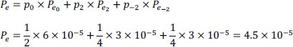
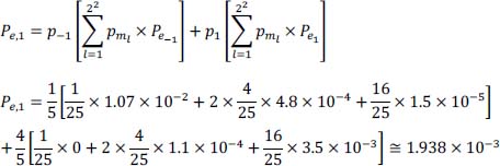
- 6) Finally, deduce the average probability of error Pe,1.
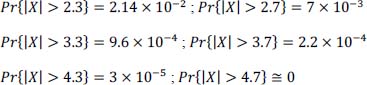
NOTE.- For a Gaussian random variable X centered (m = 0) and reduced (σ = 1) we will assume that we have approximately:
- 7) Calculate the average probability of error Pe,0 that we would have had (with the same ratio
 at the output of the equalizer) if the intersymbol interference had been canceled.
Solution of problem 21
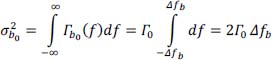
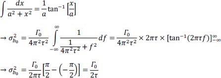
- 1) The power spectral density is:
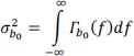
The noise power b0 (t) is ![]() given by:
given by:

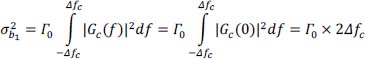
The power of the noise b1 (t) is ![]() given by:
given by:
- 2) The signal transmitted se (t) is:

The signal received sr (t) is:
with:
The signal y (t) is the response of the channel to the basic pulse (rectangular shape) x (t) , of duration θ, in the noiseless case.
The equalized signal (corrected) sc (t) is:
with:
The noise b1 (t) is the result of noise b0 (t) filtering by the equalizer whose impulse response is gc (t).
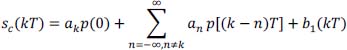
At sampling times tk = kT, the signal sc (t) is written:
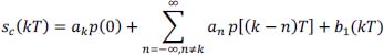
The term akp (0) represents the useful response of the system (channel + equalization) to the transmission of the symbol ak associated with the time interval kT.
The term ![]() is the intersymbol interference. It is a disturbing signal depending on all of the symbols transmitted {an}, except for the symbol ak which is related to the time interval considered.
is the intersymbol interference. It is a disturbing signal depending on all of the symbols transmitted {an}, except for the symbol ak which is related to the time interval considered.
The term b1 (kT) is the noise at the time of decision.
- 3) The messages of only the form ml = [ak–1, ak+1] interferes with symbol ak thus:
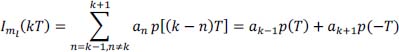
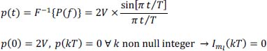
Iml (kT) depends on p [(k – n) T] , here on p (± T) . We must first calculate p (t) from P (f).

By definition, we have: p (t) = F–1 {P (f)} , hence:

This gives:
and:
Table 2.8. Intersymbol interference: amplitudes and probabilities
| ml = [ak–1,+ ak+1 ] | pml | ||
|---|---|---|---|
| -1 | -1 | V/3 | |
| -1 | 1 | 0 | |
| 1 | -1 | 0 | |
| 1 | 1 | –V/3 | |
- 4) The two expressions of conditional probabilities of error are:
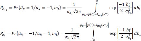
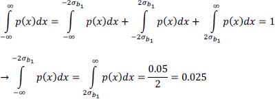
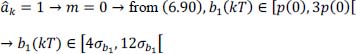
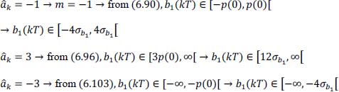
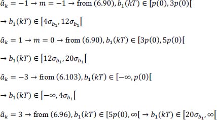
- 5) To calculate these conditional probabilities for each message ml, it is necessary to express the integration domains as a function of σb1. As:

Furthermore:
hence the following Table 2.9.
Table 2.9. Conditional probabilities of error with intersymbol interference

- 6) The average probability of error Pe,1 is given by:
- 7) As there is no intersymbol interference, this means that the first Nyquist frequency criterion is verified (α = 0) . So, from the previous results we get:
The two simplified expressions of conditional probabilities of error are now:
The two simplified expressions of conditional probabilities of error are now:
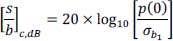
As we have the same signal-to-noise ratio as before, it means that:
And we can keep (as the approximation remains rather good) the value of the optimal threshold μ0 as a function of the noise power ![]() :
:
Thus, in this case, the previous Table 2.9 is replaced by Table 2.10:
Table 2.10. Conditional probabilities of error without intersymbol interference
| µ0 + p(0) | Pe–1 | µ0 – p(0) | Pe1 |
|---|---|---|---|
| 3.3 σb1 | ≅ 4.8 × 10⁻⁴ | –3.7 σb1 | ≅ 1.1 × 10⁻⁴ |
Finally, we get:

Thus, in this case (with the same signal-to-noise ratio), the probability of transmission error without intersymbol interference is approximately 10 times lower than it was in the presence of intersymbol interference.
2.7. Problem 22 – Baseband digital transmission (2)
The following baseband digital transmission system (Figure 2.29) is considered for the transmission of binary information.
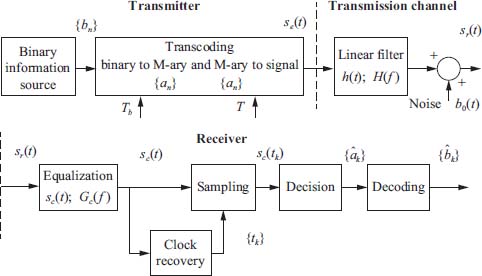
Figure 2.29. Block diagram of the baseband digital transmission system
The source of information produces a random sequence {bn} of equiprobable and independent binary variables. The coding of binary information {bn} into information symbol {an} corresponds to the following assignment:
The symbols an of information to be transmitted are supplied to the transmitter at a rate of 1/T. The coder information to signal generates a transmitted signal se (t) given by:
where x (t) is a rectangular signal of amplitude V and duration T/2.
The transmission channel is modeled by a linear filter whose impulse response is denoted by h (t) (the propagation delay here is not taken into account) and an additive degradation noise b0 (t) at the transmission channel output.
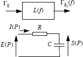
The noise b0 (t) is modeled by the low pass filtering of a white noise, of constant power spectral density Γ0. This low pass filter is considered as a first-order low pass R-C filter whose frequency gain is denoted by L (f). The noise b0 (t) is assumed, to be a second-order stationary Gaussian random process with zero mean, and independent of the useful signal. We called ![]() its average power and Γb0 (f) its power spectral density.
its average power and Γb0 (f) its power spectral density.
A receiver makes it possible to retrieve the binary information from the signal received at the output of the channel according to the block diagram from Figure 2.29. The channel equalization is produced by a linear filter of impulse response gc (t) and complex gain Gc (f) . The clock recovery, supposed to be faultless, produces a sequence of decision instants {tk} of the form tk = t0 + kT (thereafter, t0 is assumed to be zero).
The decision system uses a given decision threshold μ0 and the decision rule is as follows:

Decoding {ȃk} → {bk} is obvious.
We denote successively (⊗: convolution product):
- 1) Determine the energy bandwidth Δfb of the noise b0 (t). This will allow us to consider in the following problem that its spectrum Γb0 (f) is constant on the frequency band [– Δfb, Δfb], and zero otherwise (see Figure 2.30)
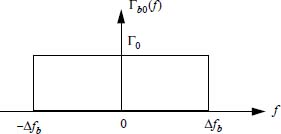
Figure 2.30. Equivalent power spectral density of noise b0 (t)
It is assumed that the equalization is of gain Gc (f) on a support fully included in the frequency band [– Δfb, Δfb] and Gc (0) =1 . We denoted Δfc as its equivalent energy bandwidth.
- 2) Determine the noise characteristics b1 (t) at the output of the equalization: the power spectral density Γb1 (f) and the power
 of the noise b1 (t) , as a function of that
  of b0 (t), its equivalent energy bandwidth Δfb and the energy bandwidth Δfc of the equalization filter.
The equalization filter is set so that the amplitude spectrum P (f) of p (t) is constant, equal to VT/α in the frequency band ![]() and equal to zero otherwise (see Figure 2.31).
and equal to zero otherwise (see Figure 2.31).

Figure 2.31. Amplitude spectrum P(f) of p(t)
- 3) Give the expression of the signal sc (tk) (made of the useful signal + intersymbol interference + noise at the instants of the form: tk = kT.
Subsequently, for sake of simplification, it will be considered that only the two symbols adjacent to a given symbol ak can interfere with it (namely symbols ak-1 and ak+1).
- 4) Which minimum value α0 of the parameter α ensures no intersymbol interference?
We then adjust the equalizer with the value α0. Under these conditions, the signal-to-noise ratio obtained at the output of the equalizer is equal to 6dB with:
- 5) Calculate the conditional probabilities of error:

knowing that we have:
Solution of problem 22
- 1) The calculation of energy bandwidth Δfb of noise b0 (t) is made from the expression of the power
 :
:
On one hand:
On the other hand, we have to calculate ![]() from the expression of Γb0 (f) , which is the result of filtering Γ0 by the first-order RC low pass filter:
from the expression of Γb0 (f) , which is the result of filtering Γ0 by the first-order RC low pass filter:
Calculation of the transfer function of a 1 st order low pass R – C filter:

For:
and:
then:
Recall:
Finally, we get:
- 2) Power spectral density Γb1 (f) and power
 of noise b1 (t).
We have:
and:
Since the support of Gc is included in [– Δfb, Δfb] then:
hence:
- 3) The equalized signal (corrected) sc (t) is:

with:
The noise b1 (t) is the result of filtering b0 (t) by the equalizer filter whose impulse response is gc (t)
At the sampling times tk = kT, the signal sc (t) is written:
The term akp (0) represents the response of the system (channel + equalization) to the transmission of the symbol ak associated with the time interval kT.
The term ![]() is the intersymbol interference.
is the intersymbol interference.
It is a disturbing signal depending on all the transmitted symbols {an } , except for the symbol ak which is related to the time interval considered.
The term b1 (kT) is the noise at the output of the equalizer at the decision instant.
- 4) Only messages in the form ml = [ak–1 , ak+1] interfere with symbol ak, so:

Iml (kT) depends on p [(k – n) T] , here on p (± T) . We have to calculate p (t) from its Fourier transform P (f) which is defined (see Figure 2.33).
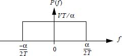
Figure 2.33. Amplitude spectrum P(f) of p(t)
We have: p (t) = F–1 {P (f)} . This gives:
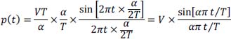
Finally, we get:
So:
This must be true for α non null integer.
- 5) Conditional probabilities of error:
Relation between V and σb1. We have
Since μ0 = 0 (equiprobable symbols) and Iml (kT) =0, then:

Knowing that:
and:
Finally we then get:
2.8. Problem 23 – M-ary baseband digital transmission
This problem deals with the baseband transmission of coded digital images over a transmission channel (cable) with reduced capacity. The different characteristics of the transmitter and receiver system in Figure 2.34 below will be analyzed together with its performances.

Figure 2.34. Block diagram of the baseband transmission system on a cable
The symbols bn are delivered by the binary source every Tb second (with the use of a buffer memory). Moreover, they are supposed to be independent and equiprobable.
The coding of binary information {bn} into information symbols {an} is done by grouping 2 bits bn to form a quaternary symbol an = {–3, – 1, 1, 3} of period T = 2Tb
The symbols an of information are provided to the transmitter at a rate of: 1/T = 10MHz
The transmitted signal se (t) is given by se (t) = ∑nanx (t – nT) where x (t) is a rectangular signal of amplitude V over the time interval [0, T [, zero elsewhere.
The transmission channel is modeled by a linear filtering whose impulse response is denoted h (t) with an additive degradation noise b0 (t) at the output of the channel. The latter is supposed to be a second-order stationary Gaussian random noise, with zero mean value, having a broad frequency bandwidth, and a mean power ![]() .
.
The equalization filter of the transmission channel works in a frequency band totally included in that of the noise. The clock regeneration is assumed to be perfectivate and provides a sequence of decision instants of the form: tk = t0 + kT
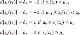
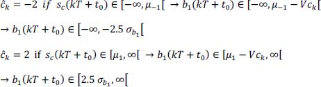
The decision system uses three thresholds, denoted μ–1 , μ0, μ1, to separate the equalized signal sc (tk) into four classes. They are given by:
We have:
We denote successively (⊗ is the convolution product):
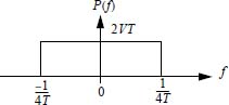
In a first phase, the equalization filter is such that the frequency gain P (f) of p (t) is constant, equal to 2VT in the frequency band [-1/4T, 1/4T] , and zero elsewhere.
- 1) Give the expression of the signal sc (tk) (composed of the useful signal + intersymbol interference + noise) at the decision instants of the form: tk = kT.
- 2) From the expression of the intersymbol interference Iml (kT) , show that only symbols a of odd-rank index [k ± (2i + 1)] interfere with symbol ak (i positive or negative integer).
Afterwards, for sake of simplification, it is considered that only the two symbols adjacent to the symbol ak interfere with it (namely ak–1 and ak+1).
- 3) By listing the different possible combinations of the message ml = [ak–1 , ak+1] interfering with ak, show that Iml (kT) can only take seven possible values that will be determined. (Afterwards, you will take π ≅ 3 as a simplification for the calculation).
Also calculate the different probabilities, each of them associated to one of the seven different values of the intersymbol interference. Here the ak will be considered equiprobable.
- 4) Show that, even without noise at the input of the receiver, the probability of ivate W error is very high.
So, we decide to perform a better equalization of the cable distortion. This second equalization is such that the frequency spectrum P (f) of p (t) is constant on the frequency band [–1/2T, 1/2T], zero elsewhere, and P (0) =2VT.
- 5) Show that the intersymbol interference is now cancelled.
Under these new conditions, we will assume that at the output of the equalizer the signal-to-noise ratio is:

- 6) Calculate the following 16 conditional probabilities:
and show that the 4x4 conditional probability matrix:
is quasi of the form given in Table 2.11:
Table 2.11. Form of the conditional probability matrix
| ak âk | - 3 | - 1 | + 1 | + 3 |
|---|---|---|---|---|
| -3 | 1 - p | p | 0 | 0 |
| -1 | p | 1 – 2 p | p | 0 |
| +1 | 0 | p | 1 – 2 p | p |
| +3 | 0 | 0 | p | 1 – p |
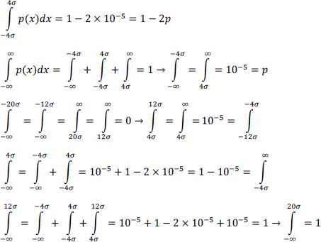
NOTE.– We will consider here that if p(x) is the probability density function of a Gaussian random variable with zero mean value:

Solution of problem 23
- 1) The transmitted signal se(t) is:
The received signal sr(t) is:
with: y(t) = x(t)⊗h(t).
The signal y(t) is the output of the channel when its input is the basic impulse (rectangular shape) x(t) of period T and without noise.
The equalized (corrected) signal sc(t) is:
with: p(t) = y(t)⊗gc(t) , that is: p(t) = x(t)⊗h(t)⊗gc(t).
The noise b1(t) is the result of filtering the noise b0(t) by the equalizer whose impulse response is gc(t).
At the sampling times tk = kT, the signal sc(t) is written:

The term akp (0) represents the useful response of the system (channel + equalization) to the transmission of the symbol ak associated with the time interval kT.
The term ![]() is the intersymbol interference.
is the intersymbol interference.
It is a disturbing signal which depends on all the symbol {an} transmitted, except for the symbol ak which is related to the time interval considered.
The term b1(kT) is the noise at the decision instant.
- 2) The intersymbol interference Iml(kT) is given by:

It depends on p [(k – n) T] , so we have to calculate p(t) from P(f)
By definition, we have: p(t) = F–1 {P(f)}, hence:
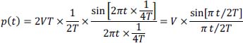
From these values, we can conclude that:
- 3) Possible values of Iml(kT).
In the case where the messages only of the form ml = [ak–1 , ak+1] interfere with the symbol ak, we have (with π ≅ 3):

Table 2.12. Interfering messages and intersymbol interference amplitude
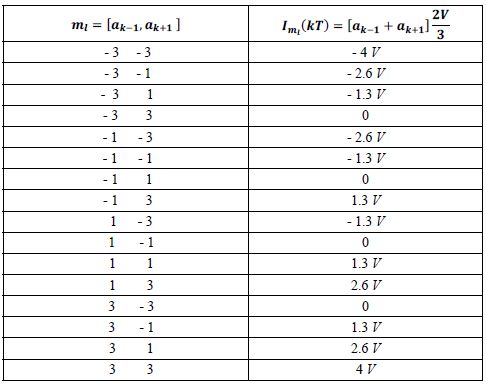
Thus, there are seven distinct values of Iml (kT).
Table 2.13. Probabilities of amplitude of intersymbol interference
| Iml (kT) | Pr{Iml (kT)} |
|---|---|
| 4 V | 1/16 |
| 2.6 V | 1/8 |
| 1.3 V | 3/16 |
| 0 | 1/4 |
| - 1.3 V | 3/16 |
| - 2.6 V | 1/8 |
| - 4 V | 1/16 |
- 4) Neglecting the noise, after equalization the signal sc(kT) is written:
The decision thresholds are given by:


Figure 2.36. Sample values akV, optimal thresholds and decision classes of ak : ȃk
It can easily be seen that to change the decision class, it is sufficient that
- – an erroneous decision on the transmitted symbol ak = 3 is made for all the values of Iml(kT) < – V, that is in 6/16 of cases;
- – similarly, an erroneous decision on the transmitted symbol ak = –3 is made for all the values of Iml(kT) > V, which is also in 6/16 cases;
- – An erroneous decision on the symbols transmitted ak = ±1 is made for all the values of |Iml(kT) | > V, that is in 12/16 of the cases.
In view of these results, even without noise, the probability of error is extremely high.
- 5) Null value of the intersymbol interference:
Under these new conditions, we have:
- 6) Calculation of the 16 following conditional probabilities:
Let us first express V as a function of ![]() and calculate the new values of the decision thresholds μ–1 , μ0, μ1:
and calculate the new values of the decision thresholds μ–1 , μ0, μ1:
At the output of the equalizer, the signal is then written:
and the threshold values of the decision blocks are:

Figure 2.37. Sample values ak2V, optimal thresholds and decision classes of ak : ȃk
The calculation of the conditional error probabilities is based on the knowledge of the noise intervals given by the course formulas (see the relations in Chapter 6 of Volume 1). For each value of the symbol ak transmitted, we have four possible decisions (three erroneous, and a correct one) on the estimated value ȃk of the symbol ak.
Recall that for the intermediate values of the symbol ak transmitted, the conditional error probability is given by:
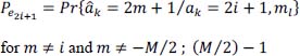
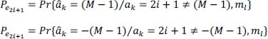
and for the extreme values of the transmitted symbol ak, the two conditional error probabilities are:
The conditional probability matrix is then obtained like this:
- – for the symbol transmitted ak = –1 → i = –1 → Pe–1, and the four decisions in reception are:
- – for the symbol transmitted ak = 1 → i = 0 → Pe1, and the four decisions in reception are:

- – for the symbol transmitted ak = 3 → i = 1 → Pe3, and the four decisions in reception are:

- – for the symbol transmitted ak = –3 → i = –2 → Pe-3, and the four decisions in reception are:
Furthermore, we have:
Hence see the matrix of conditional decision probabilities in Table 2.14 below.
Table 2.14. Conditional decision probability matrix
| ak âk | - 3 | - 1 | + 1 | + 3 |
|---|---|---|---|---|
| -3 | 1 – p | p | 0 | 0 |
| -1 | p | 1 – 2 p | p | 0 |
| +1 | 0 | P | 1 – 2 p | p |
| +3 | 0 | 0 | p | 1–p |
2.9. Problem 24 – Baseband digital transmission of bipolar coded information
We consider the transmission of information (speech) in digital form on a twowire cable transmission channel. The on-line code used is the bipolar code. The block diagram of the transmission system is shown in Figure 2.38.
The source produces a series of independent but not equiprobable binary sequence {bn}, with:
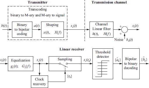
Figure 2.38. Practical chain of a digital baseband communication system with bipolar code
The transmitted signal is given by: se(t) = ∑nanx(t – nT)
The signal x(t) is a pulse of amplitude V on the time interval [0, T/2 [. The additive noise b0(t) is assumed to be stationary, Gaussian and centered, with a very broad power spectral density Γb0(f) compared to that of the signal (energy bandwidth equal to Δfb) and an average power ![]() .
.
- 1) Cite two major reasons that digital information transmissions are superior to analog transmissions.
- 2) What is the bandwidth of the standard telephone channel? And what is the maximum possible bitrate of a digital signal transmitted through this channel?
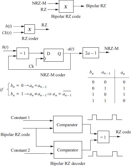
- 3) Give the transformation rule which allows us to transcode the binary symbol bn into the ternary symbol an (bipolar code).
- 4) Considering that the first non-zero symbol transmitted is always positive, what is the sequence {an} resulting from the bipolar coding of the following binary sequence {bn} of length 16 in Table 2.15.
Table 2.15. Generation of the sequence {an} of the bipolar code
| {bn} | 1 | 0 | 0 | 1 | 1 | 0 | 1 | 0 | 1 | 1 | 1 | 0 | 0 | 0 | 1 | 0 |
| {an} |
- 5) What is the advantage of using a bipolar code in baseband transmission (cite at least two reasons)?
- 6) What is the limitation? How do we bypass this limitation to prevent the coding of four consecutive null symbols b from leading to the absence of pulses in the on-line code, while ensuring that the system is operating correctly on reception?
- 7) Draw the diagram of realization of the RZ bipolar encoder and decoder.
- 8) What is the purpose of equalization? What does the Nyquist frequency criterion express?
- 9) Assuming that the equalization filter Gc(f) has a unit gain at zero frequency, determine the power
 of the noise at the decision level based on that of the observation noise and the equivalent energy bandwidth Δfc of the equalization filter.
 - 10) Give the number and value(s) of the decision threshold(s) μ of the bipolar code.
In the rest of the problem, it will be considered that the equalization is not perfect and that actually, the amplitude spectrum of the signal p(t) at the output of the equalizer, denoted P(f) , when a single impulse x(t) is sent by the transmitter and without considering the noise, is constant, equal to VT on the frequency domain [– (1 + α)/2T, (1 + α)/2T] , and zero elsewhere, with α = 0.1.
So we have: p(t) = x(t)⊗h(t)⊗gc(t).
- 11) Give the expression of the signal p(t) and its particular values at times t = 0 and t = ± T (We shall consider for simplification that sin [π (1 – α)]/π ≅ 0.1).
Similarly and for simplicity, intersymbol interference will only be considered as that resulting from the two symbols ak–1 and ak+1 adjacent to symbol ak.
- 12) Give the expression of the equalized signal sc(kT) for the kth instant of decision by showing the different contributions to the amplitude of this signal.
- 13) Determine for each possible value of ak the possible messages ml = [ak–1 , ak+1] and their conditional probabilities p(ml/i) = Pr { ml/ak = i } , according to Tables 2.16 and 2.17.
- 14) Give the expression of the probability pml and its value for each message ml. Activate Give also the amplitude of the intersymbol interference Iml of each message.
- 15) Deduce the different possible values of intersymbol interference and the associated probabilities.
Table 2.16. Possible messages ml for each ak
| ml= [ak–1, ak+1 ] | |||||||
| ak = –1 | |||||||
| ak = 0 | |||||||
| ak = 1 |
Table 2.17. Conditional probabilities Pr{ml / ak} of messages ml
| ml= [ak–1, ak+1 ] | Pr{ml/ak= –1} | Pr{ml/ak= 0} | Pr{ml/ak= 1} |
|---|---|---|---|
| m1( , ) | |||
| m2( , ) | |||
| m3( , ) | |||
| m4( , ) | |||
| m5( , ) | |||
| m6( , ) | |||
| m7( , ) | |||
| m8( , ) | |||
| m9( , ) |
Table 2.18. Probability pml and value of the intersymbol interference for each message ml
| ml= [ak–1, ak+1 ] | pml | Iml |
|---|---|---|
| m1( , ) | ||
| m2( , ) | ||
| m3( , ) | ||
| m4( , ) | ||
| m5( , ) | ||
| m6( , ) | ||
| m7( , ) | ||
| m8( , ) | ||
| m9( , ) |
Table 2.19. Possible values of inter-symbol interference and associated probabilities
| Iml | I–2 | I–1 | I0 | I1 | I2 |
|---|---|---|---|---|---|
| Value of Iml | |||||
| Pr{Iml} |
- 16) Give the expression of the probability of error Pe,a on the symbols of the bipolar code.
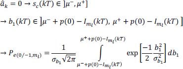
To simplify, it is considered that only the errors âk of the following type: "the decided values are adjacent to the prior value ak", are of non-zero probability:

- 17) Give the expression of each of these four conditional probabilities of possible errors (by specifying the intervals of the noise amplitude):

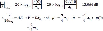
It is assumed that at the output of the equalization, the signal-to-noise ratio is:
- 18) For each message ml, calculate the intervals of the noise dynamics and the values of the conditional probability of errors according to Table 2.20 (based on the table of a centered and reduced Gaussian law).
NOTE.–
- –ul : upper limit of the interval of the noise amplitude.
- – ll: lower limit of the interval of the noise amplitude.
Table 2.20. Noise dynamics interval and conditional error probabilities
| ml | m1 | m2 | m3 | m4 | m5 | m6 | m7 | m8 | m9 |
|---|---|---|---|---|---|---|---|---|---|
| ul = ll= |
|||||||||
| Pe(–1/0,ml) | |||||||||
| ul = ll = |
|||||||||
| Pe(1/0,ml) | |||||||||
| ul = ll = |
|||||||||
| Pe(0/–1,ml) | |||||||||
| ul = ll = | |||||||||
| Pe(0/1,ml) |
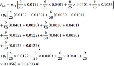
- 19) Deduce the value of the error probability Pe,a.
- 20) What would be the value of the probability of error Pe1,a, if we kept, for each of the possible values of ak, only the configuration ml leading to the most unfavorable value of the intersymbol interference Iml ?
- 21) Give the expression and the value of the probability of error Pe,b on the binary symbols decoded, under the same conditions of question 20 .
- 22) What would be the value of the probability of error Pe2,a, if there was no more intersymbol interference?
Solution of problem 24
- 1) Major reasons:
- – integration of services, therefore lower costs;
- – performance in terms of error / distortion not cumulable, because the regeneration of signals can be exactly performed.
- 2) The frequency bandwidth of the standard telephone channel is:
The maximum possible symbol rate (according to Nyquist criterion) is:
The maximum possible bitrate is:
If coding on two levels, then:
NOTE.– Usually, one uses a M-ary coding system with M ⪢ 2 where the number M is a function of the signal-to-noise ratio at the input of the decision block which ensures a probability of a wrong decision lower than a given level of admissible errors.
- 3) Rule of transformation of a binary symbol into a ternary symbol (bipolar code).
The bipolar code is a three-level code such as:

- 4) Generation of the sequence {an} (bipolar code).
| {bn} | 1 | 0 | 0 | 1 | 1 | 0 | 1 | 0 | 1 | 1 | 1 | 0 | 0 | 0 | 1 | 0 |
| {an} | 1 | 0 | 0 | -1 | 1 | 0 | -1 | 0 | 1 | -1 | 1 | 0 | 0 | 0 | -1 | 0 |
- 5) The interests in using a bipolar code in baseband transmission are:
- – no continuous component;
- – the spectrum of the transmitted signal vanishes at all the multiples of 1/Tb and limitation of the spectral occupation.
- 6) Bipolar code limitation:
If we have a long series of bits at zero, then there are no pulses issued over a period that can be significant. This causes the loss of clock synchronization at the receiver side. To overcome this drawback, the bipolar code with a high pulse density is used.
If on a period of 4Tb, there are no pulses, we have to use the HDB– 3 code.
- 7) Block diagram of the RZ bipolar encoder and decoder.
- 8) The ultimate goal of equalization is to cancel the influence of the transmission channel in order to have an ISI as small as possible (and even null).
The Nyquist frequency criterion states that the equalization must ensure that we have:
- 9) The noise power b1(t) is:
The power spectral density b1(t) is given by:
The noise power b0(t) is:
hence:
and:
- 10) Number and value(s) of the decision threshold(s) of the bipolar code: two decision thresholds, denoted: μ+ = – μ- = p (0)/2
- 11) Expression of the signal p(t) obtained by the inverse Fourier transform of the amplitude spectrum P(f).


- 12) Expression of the received and corrected signal:
with:
hence:
- 13) For each possible value of ak, determination of possible interfering messages and their conditional probabilities: p(ml/i) = Pr{ ml/ak = i }.
| ml= [ak–1, ak+1 ] | |||||||
| ak = –1 | 0 0 | 0 1 | 1 0 | 1 1 | |||
| ak = 0 | 0 0 | 0 -1 | 0 1 | -1 0 | -1 1 | 1 0 | 1 -1 |
| ak = 1 | 0 0 | 0 -1 | -1 0 | -1 -1 |
Table 2.23. Conditional probabilities: p(ml /–1)= Pr{ml / ak = –1}
| {ml/ak = –1} ml= [ak–1, ak+1 ] | p(ml/–1)= Pr{ml/ak= –1} |
|---|---|
| 0 0 | Pr{bk–1= 0, bk+1= 0} = 4/25 |
| 0 1 | Pr{bk–1 = 0, bk+1= 1} = 6/25 |
| 1 0 | Pr{bk–1 = 1, bk+1 = 0} = 6/25 |
| 1 1 | Pr{bk–1 = 1, bk+1 = 1} = 9/25 |
Table 2.24. Conditional probabilities: p(ml /–0)= Pr{ml / ak = o}
| {ml/ak = 0} ml = [ak–1, ak+1 ] | p(ml/0) = Pr{ml–ak = 0} |
|---|---|
| 0 0 | Pr{bk–1 = 0, bk+1 = 0} = 4/25 |
| 0 1 | Pr{bk–1 = 0, bk+1 = 1 and ak+1 > 0} = 6/50 |
| 0 -1 | Pr{bk–1 = 0, bk+1 = 1 and ak+1 < 0} = 6/50 |
| 1 0 | Pr{bk–1 = 1, bk+1 = 0 and ak–1 > 0} = 6/50 |
| 1 -1 | Pr{bk–1 = 1, bk+1 = 1 and ak–1 > 0} = 9/50 |
| -1 0 | Pr{bk–1 = 1, bk+1 = 0 and ak–1 < 0} = 6/50 |
| -1 1 | Pr{bk-1 = 1, bk+1 = 1 and ak–1 < 0} = 9/50 |
Table 2.25. Conditional probabilities: p(ml / 1)=Pr{ml / ak=1}
| {ml/ak = 1} ml = [ak–1, ak+1 ] | p(ml/1) = Pr{ml–ak = 1} |
|---|---|
| 0 0 | Pr{bk–1 = 0, bk+1 = 0} = 4/25 |
| 0 -1 | Pr{bk–1 = 0, bk+1 = 1} = 6/25 |
| -1 0 | Pr{bk–1 = 1, bk+1 = 0} = 6/25 |
| -1 -1 | Pr{bk–1 = 1, bk+1 = 1} = 9/25 |
The summary of all these values is given in Table 2.26.
Table 2.26. Conditional probabilities: p(ml/i) = Pr{ ml/ak = i }
| ml = [ak–1, ak+1 ] | Pr{ml/ak = –1} | Pr{ml/ak = 0} | Pr{ml/ak = 1} |
|---|---|---|---|
| m1 = (0, 0) | 4/25 | 4/25 | 4/25 |
| m2 = (0, 1) | 6/25 | 6/50 | |
| m3 = (0, –1) | 6/50 | 6/25 | |
| m4 = (1, 0) | 6/25 | 6/50 | |
| m5 = (1, –1) | 9/50 | ||
| m6 = (–1, 0) | 6/50 | 6/25 | |
| m7 = (–1, 1) | 9/50 | ||
| m8 = (–1, –1) | 9/25 | ||
| m9 = (1, 1) | 9/25 |
- 14) Expression of the probability pml:
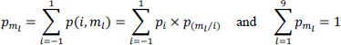
Table 2.27. Intersymbol interference amplitudes and associated probabilities with each possible interfering message
| ml = [ak–1, ak+1 ] | pml | Iml |
|---|---|---|
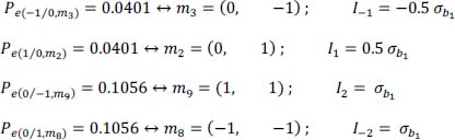
| m1 = (0, 0) | 3/10 × 4/25 + 2/5 × 4/25 + 3/10 × 4/25 = 4/25 | 0 |
| m2 = (0, 1) | 3/10 × 6/25 + 2/5 × 6/50 = 3/25 | V/10 |
| m3 = (0, –1) | 2/5 × 6/50 + 3/10 × 6/25 = 3/25 | –V/10 |
| m4 = (1, 0) | 3/10 × 6/25 + 2/5 × 6/50 = 3/25 | V/10 |
| m5 = (1, –1) | 2/5 × 9/50 = 1.8/25 | 0 |
| m6 = (–1, 0) | 2/5 × 6/50 + 3/10 × 6/25 = 3/25 | –V/10 |
| m7 = (–1, 1) | 2/5 × 9/50 = 1.8/25 | 0 |
| m8 = (–1, –1) | 3/10 × 9/25 = 2.7/25 | –V/5 |
| m9 = (1, 1) | 3/10 × 9/25 = 2.7/25 | V/5 |
with:
and we actually have:

- 15) Possible values of intersymbol interference and associated probabilities.
Table 2.28. Inter-symbol interference values and associated probabilities
| Iml | I–2 | I–1 | I0 | I1 | I2 |
|---|---|---|---|---|---|
| Value of Iml | –V/5 | –V/10 | 0 | V/10 | V/5 |
| Pr{Iml } | 1/9 | 2/9 | 3/9 | 2/9 | 1/9 |
And we have:
- 16) Expression of the probability of error on the symbols a:
- 17) Expression of each of the four conditional probabilities of possible error.
The corrected and sampled signal is:
The decision thresholds are such that:

Figure 2.41. Sample values without ISI and noise, optimal thresholds and decision classes of ak : âk
The noise b1(kT) is written:
If:
Then, we have:
- – Case of transmission ak = 0.
If we decide:

If we decide:
- – Case of transmission ak = –1.
If we decide:
- – Case of transmission ak = 1.
If we decide:

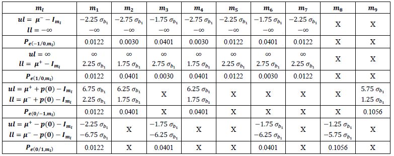
- 18) For each message ml, calculation of intervals of noise dynamics and values of the conditional probabilities of error, are given in Table 2.29.
The noise amplitude intervals should be expressed as a function of σb1. We have:
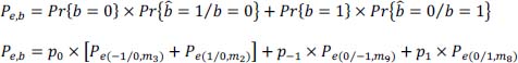
- 19) Calculation of the probability of error Pe,a :
- 20) We keep only the most unfavorable case of intersymbol interference according to the table giving the values of the conditional probabilities for each message:
hence:
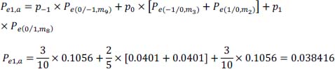
Table 2.29. Noise interval dynamics and associated probabilities according to the intersymbol interference amplitude
- 21) Expression and value of the probability of error Pe,b:
therefore: Pe,b = Pe1,a.
This result was predictable with the simplification of the statement because:
But these errors on ak do not introduce errors on bk, hence: Pe,b = Pe1,a.
- 22) Probability of error Pe2,a in the absence of ISI. We have:

hence:
We have, from the normalized Gaussian law table:
2.10. Problem 25 – Baseband transmission and reception using a partial response linear coding (1)
The problem of baseband transmitting and receiving independent binary information on a reduced capacity channel is considered.
The transmission and reception system in question uses partial response linear coding according to the Figure 2.42.

Figure 2.42. Baseband transmission and reception chain with partial response linear coder
Where

The partial response linear coding used in this problem is the NRZ duobinary coding, characterized by its transfer function:
Where D is the delay operator T (time slot allocated to the transmission of a symbol ck).
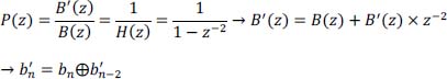
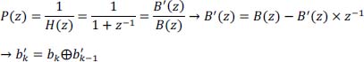
- 1) Give the transfer function P(z) of the precoder filter as well as its equation providing
 as a function of bk.
 - 2) Give the equation of the encoder generating ck from ak.
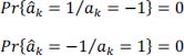
- 3) Give the relationships allowing us to estimate the binary symbols emitted
 from the symbols received ck : ĉk with and without precoding. Comment on each case.
 - 4) Give the block diagram of the precoder, transcoder and duobinary combined encoder.
The shaping filter has an impulse response x(t) considered as an NRZ signal of duration T and amplitude V.
Let us take the 14 -bit {bk} time sequence shown in Figure 2.43 (time running from left to right).
- 5) Determine (temporal representations will be plotted directly in Figure 2.43):
- – the time sequence
 associated with the output of the precoder (the latter is considered initialized to zero);
 - – the corresponding temporal sequences {ak}, {ck},
 and signal se(t).
- – the time sequence
The transmission channel is modeled by a linear filtering and additive noise at the output of the channel. The latter is a stationary second-order Gaussian noise, with a zero mean and a broad spectrum.
We assume that at the output of the equalizer, the signal-to-noise ratio obtained is:
First, we consider the classical baseband transmission system (without precoding and coding).
- 6) Give the expression of the signal sc(kT + t0) at the input of the decision unit according to the symbols a.
Take the case of the duobinary partial response transmission and reception system.
- 7) Particularize the expression of the signal sc(kT + t0).
We assume for the rest of the problem that: p(T + t0) = p(t0) = V.
- 8) Deduce the new expression of sc(kT + t0) according to the symbols ck.
- 9) Calculate the conditional probabilities of error:

- 10) Deduce the total probability of error: Pe = Pr{ĉk ≠ ck} with: ck = {2, – 2, 0}.
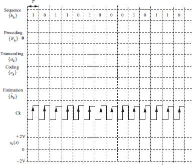
Figure 2.43. Temporal diagrams of duobinary coding and decoding
NoTE.– If X is a Gaussian random process, with mean value m and standard deviation σ, you will take:

Solution of problem 25
- 1) Transfer function P(z) of the precoder and equation giving
 as a function of bk:
- 2) Equation of the coder giving ck as a function of ak:

- 3) Equation allowing the estimation of the emitted symbols
 from the received symbols ck : ĉk.
With precoding, the transcoder provides:
hence:
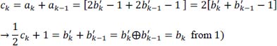
Thus, we get a direct estimation of the emitted sequence {bk} from the received sequence {ĉk}.
Without precoding:
This leads to a propagation of decision errors. Indeed, if bk–1 is badly decoded, it will also be the case for bk.
- 4) Block diagram of the precoder, transcoder and duobinary coder.

Figure 2.44. Duobinary precoder, transcoder and coder scheme
- 5) Chronograms of duobinary coding and decoding.

Figure 2.45. Chronograms of duobinary coding and decoding. For a color version of this figure, see www.iste.co.uk/assad/digita/2.zip
- 6) Expression of the signal sc(kT + t0):
- 7) Duobinary partial response transmission and reception system: expression of sc(kT + t0).
With p(T + t0) = p(t0) = V, the intersymbol interference is now given by:

- 8) New expression of sc(kT + t0):
- 9) Conditional probabilities of error:
From the result obtained in response 8, we have:

The decision thresholds are located in the middle of two adjacent levels obtained without noise:
Let’s express the decision thresholds according to σb1:

Figure 2.46. Values of sample ckV, optimum thresholds and decision classes of ck : ĉk
We have three possible decision values of symbol ĉk one without errors and two with errors.
Transmission of ck = 2, we decide on reception:

Transmission of ck = 0, we decide on reception:
Transmission of ck =–2, we decide on reception:

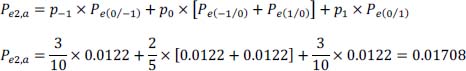
- 10) Calculation of the total probability of error:
The total probability of error is then given by:
The binary symbols bk are independent and identically distributed on the alphabet {0,1}, hence:
The probabilities of transmitting the symbols ck are respectively:
Hence, the total probability of error:

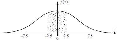
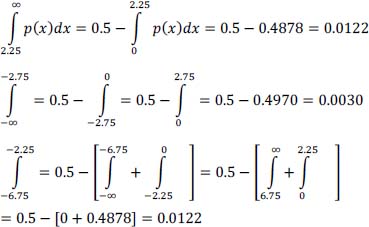
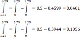
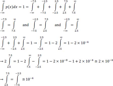
Figure 2.47. Gaussian probability law and distribution intervals
Calculation of integrals:
2.11. Problem 26 – Baseband transmission and reception using a partial response linear coding (2)
The problem of transmitting and receiving independent binary information on a reduced capacity channel is considered. The baseband transmission and reception system in question uses the partial response linear coding according to the following Figures 2.48 and 2.49.

Figure 2.48. Partial response transmitter and receiver block diagram

Figure 2.49. Details of the partial response transmitter block diagram
with:

The partial response linear coding used in this problem is defined by the two following transfer functions:
The transmission channel is modeled by a linear filtering and additive noise at the output of the channel. Noise is considered as a second-order stationary, Gaussian random process, with zero mean and broad spectrum.
- 1) Give the transfer function of the encoder filter H(z).
- 2) Give the transfer function of the precoder filter P(z) as well as its equation providing
 as a function of bk.
 - 3) Give the equation of the encoder providing ck as a function of ak.
- 4) Give the relationships providing the estimation of the transmitting symbols bk from the received symbols ĉk with and without precoding. Comment on each case.
- 5) Give the implementation scheme of the precoder, transcoder and combined encoder.
The shaping filter has an impulse response x(t) considered as an NRZ signal of duration T and amplitude V/2.
Let us take the 14 -bit sequence {bk} shown in Table 2.30 (time running from left to right).
- 6) Determine (the temporal diagrams will be given in Table 2.30):
- – the time sequence
 associated with the output of the precoder (the latter is considered initialized to zero);
 - – the corresponding time sequences {ak}, {ck},
 and plot the signal se(t).
- – the time sequence
We assume that at the output of the equalizer, the signal-to-noise ratio obtained is:
We first consider the classical baseband transmission system (without precoding and coding).
- 7) Give the expression of the signal sc(kT) at the input of the decision unit.
In the case of the partial response transmission and reception system defined in Figure 2.48.
- 8) Particularize the expression of sc(kT).
Assuming that: p (3T) = p (0) = V.
- 9) Deduce the new expression of sc(kT) according to, in particular, the symbols ck.
- 10) Calculate the conditional probabilities of error:

- 11) Deduce the total probability of error:

NoTE.– If X is a Gaussian random process, with mean value m and standard deviation σ, you will take:
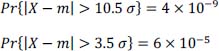
Table 2.30. Temporal representation of the proposed partial response coding and decoding system
| {bk} | 1 | 0 | 0 | 1 | 0 | 1 | 1 | 1 | 0 | 1 | 0 | 0 | 1 | 0 | |||
| 0 | 0 | 0 | |||||||||||||||
| {ak} | |||||||||||||||||
| {ck} | |||||||||||||||||
| se(t) |
Solution of problem 26
- 1) Transfer function of the encoding filter:

- 2) Transfer function of the precoder:

- 3) Equation defining the encoder:

- 4) Equation giving the estimate of bk.
With precoding, the transcoder gives: ![]() hence:
hence:
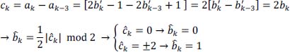
So a direct estimate of the sequence {bk} issued from the sequence {ck} received.
Without precoding:
This leads to a propagation of decision errors. Indeed, if bk-3 is badly decoded, it will be also the same case for bk.
- 5) Block diagram of the combined precoder, transcoder and encoder:

Figure 2.50. Combined scheme of precoder, transcoder and encoder
- 6) Temporal sequences:
Table 2.31. Temporal sequences. For a color version of this table, see www.iste.co.uk/assad/digita/2.zip

- 7) Expression of the signal sc(kT):
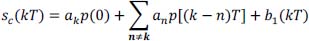
- 8) In this case, the intersymbol interference is:
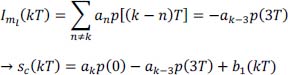
- 9) In this particular case, we have:

- 10) The different conditional probabilities of errors are as follows:
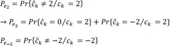
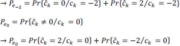
- a) Calculation of conditional probabilities of errors. According to the result obtained in question 9, we have:
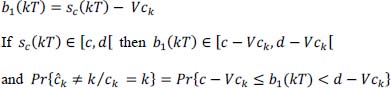
The decision thresholds [c, d [ are such that:

Let’s express the decision thresholds according to σb1:

Figure 2.51. Values of sample ckV, optimum thresholds and decision classes of ck : ĉk
- b) Application of the decision rules. We have three possible decision values on ck, one without errors and two with errors.
- c) Transmission of symbol ck = 2, we decide on reception:
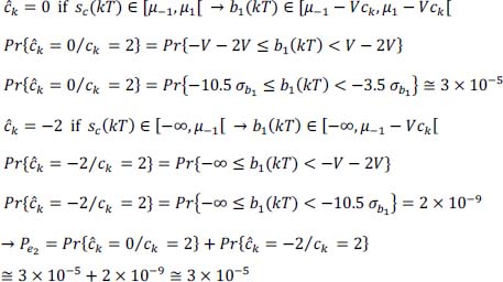
- d) Transmission of symbol ck=0, we decide on reception:
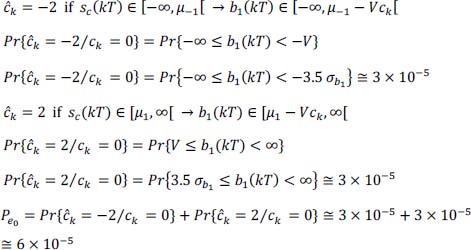
- e) Transmission of symbol ck=–2, we decide on reception:

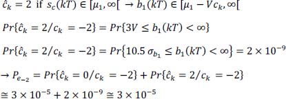

Figure 2.52. Gaussian probability law with zero mean and unit standard deviation, and distribution intervals
Calculation of integrals:

- 11) The total probability of error is then:
The symbols bk are independent and identically distributed on the alphabet {0,1}, hence:
The probabilities of emission of the symbols ck are:
Hence finally: