
The Fast Fourier Transform
There are several ways to calculate the discrete Fourier transform (DFT), such as solving simultaneous linear equations or the correlation method described in Chapter 8. The Fast Fourier Transform (FFT) is another method for calculating the DFT. While it produces the same result as the other approaches, it is incredibly more efficient, often reducing the computation time by hundreds. This is the same improvement as flying in a jet aircraft versus walking! If the FFT were not available, many of the techniques described in this book would not be practical. While the FFT only requires a few dozen lines of code, it is one of the most complicated algorithms in DSP. But don’t despair! You can easily use published FFT routines without fully understanding the internal workings.
Real DFT Using the Complex DFT
J.W. Cooley and J.W. Tukey are given credit for bringing the FFT to the world in their paper: “An algorithm for the machine calculation of complex Fourier Series,” Mathematics Computation, Vol. 19, 1965, pp 297−301. In retrospect, others had discovered the technique many years before. For instance, the great German mathematician Karl Friedrich Gauss (1777–1855) had used the method more than a century earlier. This early work was largely forgotten because it lacked the tool to make it practical: the digital computer. Cooley and Tukey are honored because they discovered the FFT at the right time, the beginning of the computer revolution.
The FFT is based on the complex DFT, a more sophisticated version of the real DFT discussed in the last four chapters. These transforms are named for the way each represents data, that is, using complex numbers or using real numbers. The term complex does not mean that this representation is difficult or complicated, but that a specific type of mathematics is used. Complex mathematics often is difficult and complicated, but that isn’t where the name comes from. Chapter 29 discusses the complex DFT and provides the background needed to understand the details of the FFT algorithm. The topic of this chapter is simpler: how to use the FFT to calculate the real DFT, without drowning in a mire of advanced mathematics.
Since the FFT is an algorithm for calculating the complex DFT, it is important to understand how to transfer real DFT data into and out of the complex DFT format. Figure 12-1 compares how the real DFT and the complex DFT store data. The real DFT transforms an N point time domain signal into two N/2 + 1 point frequency domain signals. The time domain signal is called just that: the time domain signal. The two signals in the frequency domain are called the real part and the imaginary part, holding the amplitudes of the cosine waves and sine waves, respectively. This should be very familiar from past chapters.
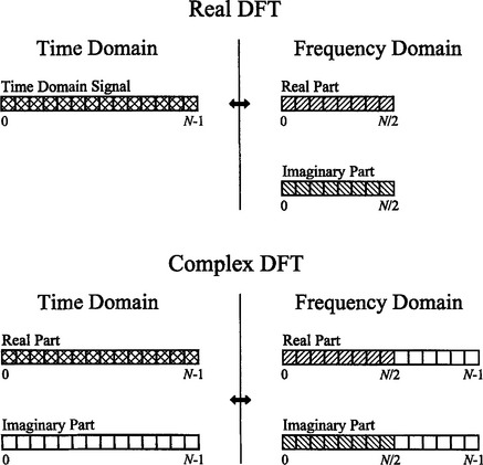
FIGURE 12-1 Comparing the real and complex DFTs. The real DFT takes an N point time domain signal and creates two N/2 + 1 point frequency domain signals. The complex DFT takes two N point time domain signals and creates two N point frequency domain signals. The crosshatched regions show the values common to the two transforms.
In comparison, the complex DFT transforms two N point time domain signals into two N point frequency domain signals. The two time domain signals are called the real part and the imaginary part, just as are the frequency domain signals. In spite of their names, all of the values in these arrays are just ordinary numbers. (If you are familiar with complex numbers: the j’s are not included in the array values; they are a part of the mathematics. Recall that the operator, Im( ), returns a real number).
Suppose you have an N point signal, and need to calculate the real DFT by means of the complex DFT (such as by using the FFT algorithm). First, move the N point signal into the real part of the complex DFT’s time domain, and then set all of the samples in the imaginary part to zero. Calculation of the complex DFT results in a real and an imaginary signal in the frequency domain, each composed of N points. Samples 0 through N/2 of these signals correspond to the real DFT’s spectrum.
As discussed in Chapter 10, the DFT’s frequency domain is periodic when the negative frequencies are included (see Fig. 10-9). The choice of a single period is arbitrary; it can be chosen between −1.0 and 0, −0.5 and 0.5, 0 and 1.0, or any other one-unit interval referenced to the sampling rate. The complex DFT’s frequency spectrum includes the negative frequencies in the 0 to 1.0 arrangement. In other words, one full period stretches from sample 0 to sample N−1, corresponding with 0 to 1.0 times the sampling rate. The positive frequencies sit between sample 0 and N/2, corresponding with 0 to 0.5. The other samples, between N/2 + 1 and N−1, contain the negative frequency values (which are usually ignored).
Calculating a real inverse DFT using a complex inverse DFT is slightly harder. This is because you need to insure that the negative frequencies are loaded in the proper format. Remember, points 0 through N/2 in the complex DFT are the same as in the real DFT, for both the real and the imaginary parts. For the real part, point N/2 + 1 is the same as point N/2−1, point N/2 + 2 is the same as point N/2−2, etc. This continues to point N−1 being the same as point 1. The same basic pattern is used for the imaginary part, except the sign is changed. That is, point N/2 + 1 is the negative of point N/2−1, point N/2 + 2 is the negative of point N/2−2, etc. Notice that samples 0 and N/2 do not have a matching point in this duplication scheme. Use Fig. 10-9 as a guide to understanding this symmetry. In practice, you load the real DFT’s frequency spectrum into samples 0 to N/2 of the complex DFT’s arrays, and then use a subroutine to generate the negative frequencies between samples N/2 + 1 and N−1. Table 12-1 shows such a program. To check that the proper symmetry is present, after taking the inverse FFT, look at the imaginary part of the time domain. It will contain all zeros if everything is correct (except for a few parts-per-million of noise, using single precision calculations).
TABLE 12-1
6000 ’NEGATIVE FREQUENCY GENERATION
6010 ’This subroutine creates the complex frequency domain from the real frequency domain.
6020 ’Upon entry to this subroutine, N% contains the number of points in the signals, and
6030 ’REX[ ] and IMX[ ] contain the real frequency domain in samples 0 to N%/2.
6040 ’On return, REX[ ] and IMX[ ] contain the complex frequency domain in samples 0 to N%−1.
6050’
6060 FOR K% = (N%/2+1) TO (N%−1)
6070 REX[K%]= REX[N%−K%]
6080 IMX[K%] = −IMX[N%−K%]
6090 NEXT K%
6100’
6110 RETURN
How the FFT Works
The FFT is a complicated algorithm, and its details are usually left to those that specialize in such things. This section describes the general operation of the FFT, but skirts a key issue: the use of complex numbers. If you have a background in complex mathematics, you can read between the lines to understand the true nature of the algorithm. Don’t worry if the details elude you; few scientists and engineers that use the FFT could write the program from scratch.
In complex notation, the time and frequency domains each contain one signal made up of N complex points. Each of these complex points is composed of two numbers, the real part and the imaginary part. For example, when we talk about complex sample X[42], it refers to the combination of Re X[42] and Im X[42]. In other words, each complex variable holds two numbers. When two complex variables are multiplied, the four individual components must be combined to form the two components of the product (such as in Eq. 9-1). The following discussion on “How the FFT works” uses this jargon of complex notation. That is, the singular terms signal, point, sample, and value refer to the combination of the real part and the imaginary part.
The FFT operates by decomposing an N point time domain signal into N time domain signals each composed of a single point. The second step is to calculate the N frequency spectra corresponding to these N time domain signals. Lastly, the N spectra are synthesized into a single frequency spectrum.
Figure 12-2 shows an example of the time domain decomposition used in the FFT. In this example, a 16-point signal is decomposed through four separate stages. The first stage breaks the 16-point signal into two signals each consisting of 8 points. The second stage decomposes the data into four signals of 4 points. This pattern continues until there are N signals composed of a single point. An interlaced decomposition is used each time a signal is broken in two, that is, the signal is separated into its even and odd numbered samples. The best way to understand this is by inspecting Fig. 12-2 until you grasp the pattern. There are Log2N stages required in this decomposition, i.e., a 16-point signal (24) requires 4 stages, a 512-point signal (27) requires 7 stages, a 4096-point signal (212) requires 12 stages, etc. Remember this value, Log2N; it will be referenced many times in this chapter.
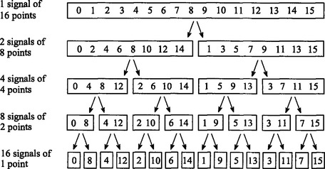
FIGURE 12-2 The FFT decomposition. An N point signal is decomposed into N signals each containing a single point. Each stage uses an interlace decomposition, separating the even and odd numbered samples.
Now that you understand the structure of the decomposition, it can be greatly simplified. The decomposition is nothing more than a reordering of the samples in the signal. Figure 12-3 shows the rearrangement pattern required. On the left, the sample numbers of the original signal are listed along with their binary equivalents. On the right, the rearranged sample numbers are listed, also along with their binary equivalents. The important idea is that the binary numbers are the reversals of each other. For example, sample 3 (0011) is exchanged with sample number 12 (1100). Likewise, sample number 14 (1110) is swapped with sample number 7 (0111), and so forth. The FFT time domain decomposition is usually carried out by a bit reversal sorting algorithm. This involves rearranging the order of the N time domain samples by counting in binary with the bits flipped left-for-right (such as in the far right column in Fig. 12-3).
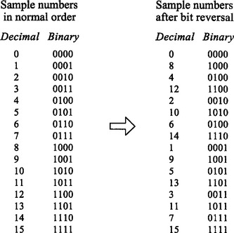
FIGURE 12-3 The FFT bit reversal sorting. The FFT time domain decomposition can be implemented by sorting the samples according to bit reversed order.
The next step in the FFT algorithm is to find the frequency spectra of the 1-point time domain signals. Nothing could be easier; the frequency spectrum of a 1-point signal is equal to itself. This means that nothing is required to do this step. Although there is no work involved, don’t forget that each of the 1-point signals is now a frequency spectrum, and not a time domain signal.
The last step in the FFT is to combine the N frequency spectra in the exact reverse order that the time domain decomposition took place. This is where the algorithm gets messy. Unfortunately, the bit reversal shortcut is not applicable, and we must go back one stage at a time. In the first stage, 16 frequency spectra (1 point each) are synthesized into 8 frequency spectra (2 points each). In the second stage, the 8 frequency spectra (2 points each) are synthesized into 4 frequency spectra (4 points each), and so on. The last stage results in the output of the FFT, a 16-point frequency spectrum.
Figure 12-4 shows how two frequency spectra, each composed of 4 points, are combined into a single frequency spectrum of 8 points. This synthesis must undo the interlaced decomposition done in the time domain. In other words, the frequency domain operation must correspond to the time domain procedure of combining two 4-point signals by interlacing. Consider two time domain signals, abcd and efgh. An 8-point time domain signal can be formed by two steps: dilute each 4-point signal with zeros to make it an 8-point signal, and then add the signals together. That is, abcd becomes a0b0c0d0, and efgh becomes 0e0f0g0h. Adding these two 8-point signals produces aebfcgdh. As shown in Fig. 12-4, diluting the time domain with zeros corresponds to a duplication of the frequency spectrum. Therefore, the frequency spectra are combined in the FFT by duplicating them, and then adding the duplicated spectra together.
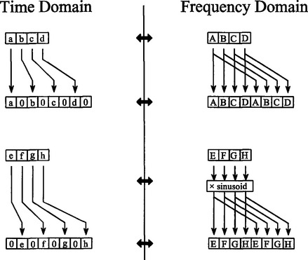
FIGURE 12-4 The FFT synthesis. When a time domain signal is diluted with zeros, the frequency domain is duplicated. If the time domain signal is also shifted by one sample during the dilution, the spectrum will additionally be multiplied by a sinusoid.
In order to match up when added, the two time domain signals are diluted with zeros in a slightly different way. In one signal, the odd points are zero, while in the other signal, the even points are zero. In other words, one of the time domain signals (0e0f0g0h in Fig. 12-4) is shifted to the right by one sample. This time domain shift corresponds to multiplying the spectrum by a sinusoid. To see this, recall that a shift in the time domain is equivalent to convolving the signal with a shifted delta function. This multiplies the signal’s spectrum with the spectrum of the shifted delta function. The spectrum of a shifted delta function is a sinusoid (see Fig 11-2).
Figure 12-5 shows a flow diagram for combining two 4-point spectra into a single 8-point spectrum. To reduce the situation even more, notice that Fig. 12-5 is formed from the basic pattern in Fig 12-6 repeated over and over.
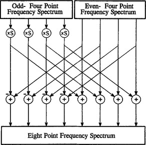
FIGURE 12-5 FFT synthesis flow diagram. This shows the method of combining two 4-point frequency spectra into a single 8-point frequency spectrum. The ×S operation means that the signal is multiplied by a sinusoid with an appropriately selected frequency.
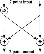
FIGURE 12-6 The FFT butterfly. This is the basic calculation element in the FFT, taking two complex points and converting them into two other complex points.
This simple flow diagram is called a butterfly due to its winged appearance. The butterfly is the basic computational element of the FFT, transforming two complex points into two other complex points.
Figure 12-7 shows the structure of the entire FFT. The time domain decomposition is accomplished with a bit reversal sorting algorithm. Transforming the decomposed data into the frequency domain involves nothing and therefore does not appear in the figure.
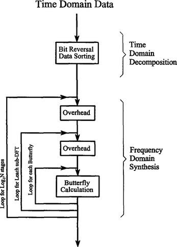
FIGURE 12-7 Flow diagram of the FFT. This is based on three steps: (1) decompose an N point time domain signal into N signals each containing a single point, (2) find the spectrum of each of the N point signals (nothing required), and (3) synthesize the N frequency spectra into a single frequency spectrum.
The frequency domain synthesis requires three loops. The outer loop runs through the Log2N stages (i.e., each level in Fig. 12-2, starting from the bottom and moving to the top). The middle loop moves through each of the individual frequency spectra in the stage being worked on (i.e., each of the boxes on any one level in Fig. 12-2). The innermost loop uses the butterfly to calculate the points in each frequency spectra (i.e., looping through the samples inside any one box in Fig. 12-2). The overhead boxes in Fig. 12-7 determine the beginning and ending indexes for the loops, as well as calculating the sinusoids needed in the butterflies. Now we come to the heart of this chapter, the actual FFT programs.
FFT Programs
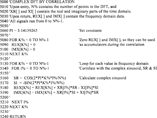
As discussed in Chapter 8, the real DFT can be calculated by correlating the time domain signal with sine and cosine waves (see Table 8-2). Table 12-2 shows a program to calculate the complex DFT by the same method. In an apples-to-apples comparison, this is the program that the FFT improves upon.
TABLE 12-2
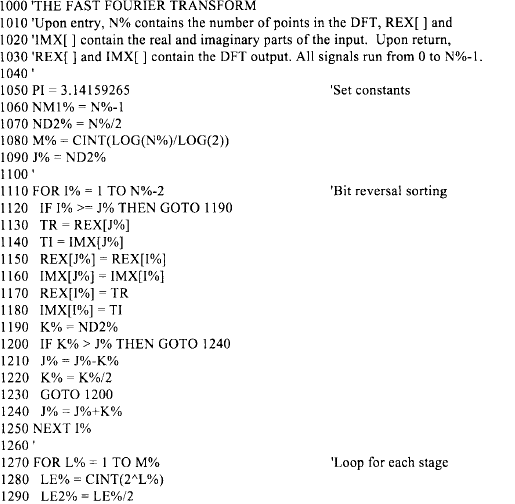
Tables 12-3 and 12-4 show two different FFT programs, one in FORTRAN and one in BASIC. First we will look at the BASIC routine in Table 12-4. This subroutine produces exactly the same output as the correlation technique in Table 12-2, except it does it much faster. The block diagram in Fig. 12-7 can be used to identify the different sections of this program. Data are passed to this FFT subroutine in the arrays: REX[ ] and IMX[ ], each running from sample 0 to N−1. Upon return from the subroutine, REX[ ] and IMX[ ] are overwritten with the frequency domain data. This is another way that the FFT is highly optimized; the same arrays are used for the input, intermediate storage, and output. This efficient use of memory is important for designing fast hardware to calculate the FFT. The term in-place computation is used to describe this memory usage.
TABLE 12-3
The Fast Fourier Transform in FORTRAN. Data are passed to this subroutine in the variables X( ) and M. The integer, M, is the base two logarithm of the length of the DFT, i.e., M = 8 for a 256 point DFT, M = 12 for a 4096 point DFT, etc. The complex array, X( ), holds the time domain data upon entering the DFT. Upon return from this subroutine, X( ) is overwritten with the frequency domain data. Take note: this subroutine requires that the input and output signals ran from X(1) through X(N), rather than the customary X(0) through X(N−1).
| SUBROUTINE FFT(X,M) | |
| COMPLEX X(4096),U,S,T | |
| PI=3.14159265 | |
| N=2**M | |
| DO 20 L=1,M | |
| LE=2**(M+1−L) | |
| LE2=LE/2 | |
| U=(1−0,0.0) | |
| S=CMPLX(COS(PI/FLOAT(LE2)),-SIN(PI/FLOAT(LE2))) | |
| DO 20 J=1,LE2 | |
| DO 10 I=J,N,LE | |
| IP=I+LE2 | |
| T=X(I)+X(IP) | |
| X(IP)=(X(I)-X(IP))*U | |
| 10 | X(I)=T |
| 20 | U=U*S |
| ND2=N/2 | |
| NM1=N−1 | |
| J=l | |
| DO 50 1=1,NM 1 | |
| IF(I.GE.J) GO TO 30 | |
| T=X(J) | |
| X(J)=X(I) | |
| X(I)=T | |
| 30 | K=ND2 |
| 40 | IF(K.GE.J) GO TO 50 |
| J=J-K | |
| K=K/2 | |
| GO TO 40 | |
| 50 | J=J+K |
| RETURN | |
| END |
While all FFT programs produce the same numerical result, there are subtle variations in programming that you need to look out for. Several of these important differences are illustrated by the FORTRAN program listed in Table 12-3. This program uses an algorithm called decimation in frequency, while the previously described algorithm is called decimation in time. In a decimation in frequency algorithm, the bit reversal sorting is done after the three nested loops. There are also FFT routines that completely eliminate the bit reversal sorting. None of these variations significantly improve the performance of the FFT, and you shouldn’t worry about which one you are using.
The important differences between FFT algorithms concern how data are passed to and from the subroutines. In the BASIC program, data enter and leave the subroutine in the arrays REX[ ] and IMX[ ], with the samples running from index 0 to N−1. In the FORTRAN program, data are passed in the complex array X( ), with the samples running from 1 to N. Since this is an array of complex variables, each sample in X( ) consists of two numbers, a real part and an imaginary part. The length of the DFT must also be passed to these subroutines. In the BASIC program, the variable N% is used for this purpose. In comparison, the FORTRAN program uses the variable M, which is defined to equal Log2N. For instance, M will be 8 for a 256-point DFT, 12 for a 4096-point DFT, etc. The point is, the programmer who writes an FFT subroutine has many options for interfacing with the host program. Arrays that run from 1 to N, such as in the FORTRAN program, are especially aggravating. Most of the DSP literature (including this book) explains algorithms assuming the arrays run from sample 0 to N−1. For instance, if the arrays run from 1 to N, the symmetry in the frequency domain is around points 1 and N/2 + 1, rather than points 0 and N/2,
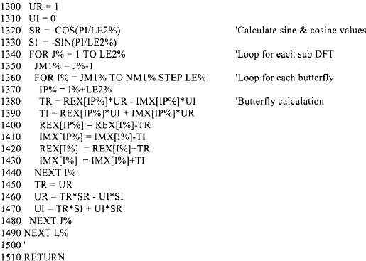
Using the complex DFT to calculate the real DFT has another interesting advantage. The complex DFT is more symmetrical between the time and frequency domains than the real DFT. That is, the duality is stronger. Among other things, this means that the inverse DFT is nearly identical to the forward DFT. In fact, the easiest way to calculate an inverse FFT is to calculate a forward FFT, and then adjust the data. Table 12-5 shows a subroutine for calculating the Inverse FFT in this manner.
TABLE 12-5
Suppose you copy one of these FFT algorithms into your computer program and start it running. How do you know if it is operating properly? Two tricks are commonly used for debugging. First, start with some arbitrary time domain signal, such as from a random number generator, and run it through the FFT. Next, run the resultant frequency spectrum through the inverse FFT and compare the result with the original signal. They should be identical, except round-off noise (a few parts-per-million for single precision).
The second test of proper operation is that the signals have the correct symmetry. When the imaginary part of the time domain signal is composed of all zeros (the normal case), the frequency domain of the complex DFT will be symmetrical around samples 0 and N/2, as previously described.
Likewise, when this correct symmetry is present in the frequency domain, the inverse DFT will produce a time domain that has an imaginary part composed of all zeros (plus round-off noise). These debugging techniques are essential for using the FFT; become familiar with them.
Speed and Precision Comparisons
When the DFT is calculated by correlation (as in Table 12-2), the program uses two nested loops, each running through N points. This means that the total number of operations is proportional to N times N. The time to complete the program is thus given by:
DFT execution time. The time required to calculate a DFT by correlation is proportional to the length of the DFT squared.
where N is the number of points in the DFT and kDFT is a constant of proportionality. If the sine and cosine values are calculated within the nested loops, kDFT is equal to about 25 microseconds on a Pentium at 100 MHz. If you precalculate the sine and cosine values and store them in a look-up-table, kDFT drops to about 7 microseconds. For example, a 1024-point DFT will require about 25 seconds, or nearly 25 milliseconds per point. That’s slow!
Using this same strategy we can derive the execution time for the FFT. The time required for the bit reversal is negligible. In each of the Log2N stages there are N/2 butterfly computations. This means the execution time for the program is approximated by:
FFT execution time. The time required to calculate a DFT using the FFT is proportional to N multiplied by the logarithm of N.
The value of kFFT is about 10 microseconds on a 100-MHz Pentium system. A 1024-point FFT requires about 70 milliseconds to execute, or 70 microseconds per point. This is more than 300 times faster than the DFT calculated by correlation!
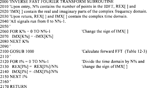
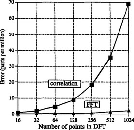
Not only is NLog2N less than N2, it increases much more slowly as N becomes larger. For example, a 32-point FFT is about ten times faster than the correlation method. However, a 4096-point FFT is one-thousand times faster. For small values of N (say, 32 to 128), the FFT is important. For large values of N (1024 and above), the FFT is absolutely critical. Figure 12-8 compares the execution times of the two algorithms in a graphical form.
FIGURE 12-8 Execution times for calculating the DFT. The correlation method refers to the algorithm described in Table 12-2. This method can be made faster by precalculating the sine and cosine values and storing them in a look-up table (LUT). The FFT (Table 12-3) is the fastest algorithm when the DFT is greater than 16 points long. The times shown are for a Pentium processor at 100 MHz.
The FFT has another advantage besides raw speed. The FFT is calculated more precisely because the fewer number of calculations results in less round-off error. This can be demonstrated by taking the FFT of an arbitrary signal, and then running the frequency spectrum through an Inverse FFT. This reconstructs the original time domain signal, except for the addition of round-off noise from the calculations. A single number characterizing this noise can be obtained by calculating the standard deviation of the difference between the two signals. For comparison, this same procedure can be repeated using a DFT calculated by correlation, and a corresponding inverse DFT. How does the round-off noise of the FFT compare to the DFT by correlation? See for yourself in Fig. 12-9.
Further Speed Increases
There are several techniques for making the FFT even faster; however, the improvements are only about 20–40%. In one of these methods, the time domain decomposition is stopped two stages early, when each signal is composed of only four points. Instead of calculating the last two stages, highly optimized code is used to jump directly into the frequency domain, using the simplicity of four point sine and cosine waves.
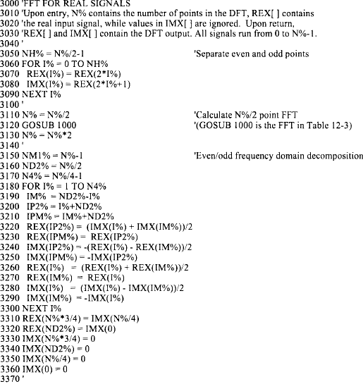
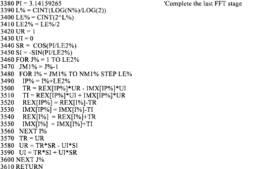
Another popular algorithm eliminates the wasted calculations associated with the imaginary part of the time domain being zero, and the frequency spectrum being symmetrical. In other words, the FFT is modified to calculate the real DFT, instead of the complex DFT. These algorithms are called the real FFT and the real inverse FFT (or similar names). Expect them to be about 30% faster than the conventional FFT routines. Tables 12-6 and 12-7 show programs for these algorithms.
TABLE 12-6
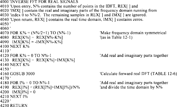
TABLE 12-7
There are two small disadvantages in using the real FFT. First, the code is about twice as long. While your computer doesn’t care, you must take the time to convert someone else’s program to run on your computer. Second, debugging these programs is slightly harder because you cannot use symmetry as a check for proper operation. These algorithms force the imaginary part of the time domain to be zero, and the frequency domain to have left-right symmetry. For debugging, check that these programs produce the same output as the conventional FFT algorithms.
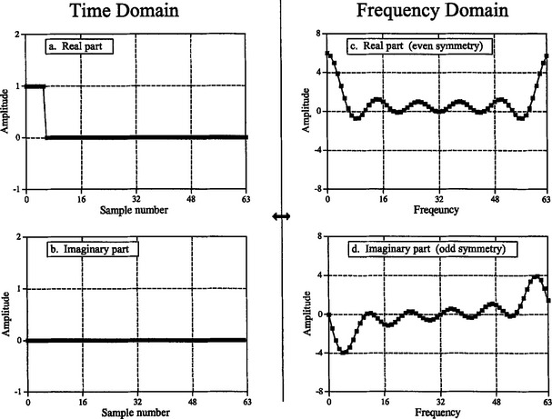
Figures 12-10 and 12-11 illustrate how the real FFT works. In Fig. 12-10, (a) and (b) show a time domain signal that consists of a pulse in the real part, and all zeros in the imaginary part. Figures (c) and (d) show the corresponding frequency spectrum. As previously described, the frequency domain’s real part has an even symmetry around sample 0 and sample N/2, while the imaginary part has an odd symmetry around these same points.
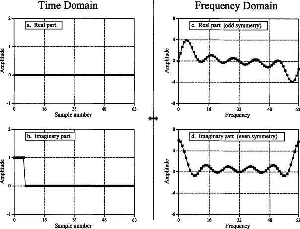
Now consider Fig. 12-11, where the pulse is in the imaginary part of the time domain, and the real part is all zeros. The symmetry in the frequency domain is reversed; the real part is odd, while the imaginary part is even. This situation will be discussed in Chapter 29. For now, take it for granted that this is how the complex DFT behaves.
What if there is a signal in both parts of the time domain? By additivity, the frequency domain will be the sum of the two frequency spectra. Now the key element: a frequency spectrum composed of these two types of symmetry can be perfectly separated into the two component signals. This is achieved by the even/odd decomposition discussed in Chapter 5. In other words, two real DFT’s can be calculated for the price of single FFT. One of the signals is placed in the real part of the time domain, and the other signal is placed in the imaginary part. After calculating the complex DFT (via the FFT, of course), the spectra are separated using the even/odd decomposition. When two or more signals need to be passed through the FFT, this technique reduces the execution time by about 40%. The improvement isn’t a full factor of two because of the calculation time required for the even/odd decomposition. This is a relatively simple technique with few pitfalls, nothing like writing an FFT routine from scratch.
The next step is to modify the algorithm to calculate a single DFT faster. It’s ugly, but here is how it is done. The input signal is broken in half by using an interlaced decomposition. The N/2 even points are placed into the real part of the time domain signal, while the N/2 odd points go into the imaginary part. An N/2 point FFT is then calculated, requiring about one-half the time as an N point FFT. The resulting frequency domain is then separated by the even/odd decomposition, resulting in the frequency spectra of the two interlaced time domain signals. These two frequency spectra are then combined into a single spectrum, just as in the last synthesis stage of the FFT.
To close this chapter, consider that the FFT is to digital signal processing what the transistor is to electronics. It is a foundation of the technology; everyone in the field knows its characteristics and how to use it. However, only a small number of specialists really understand the details of the internal workings.