
The Discrete Fourier Transform
Fourier analysis is a family of mathematical techniques, all based on decomposing signals into sinusoids. The discrete Fourier transform (DFT) is the family member used with digitized signals. This is the first of four chapters on the real DFT, a version of the discrete Fourier transform that uses real numbers to represent the input and output signals. The complex DFT, a more advanced technique that uses complex numbers, will be discussed in Chapter 31. In this chapter we look at the mathematics and algorithms of the Fourier decomposition, the heart of the DFT.
The Family of Fourier Transform
Fourier analysis is named after Jean Baptiste Joseph Fourier (1768–1830), a French mathematician and physicist. (Fourier is pronounced: for·ē·![]() , and is always capitalized). While many contributed to the field, Fourier is honored for his mathematical discoveries and insight into the practical usefulness of the techniques. Fourier was interested in heat propagation, and presented a paper in 1807 to the Institut de France on the use of sinusoids to represent temperature distributions. The paper contained the controversial claim that any continuous periodic signal could be represented as the sum of properly chosen sinusoidal waves. Among the reviewers were two of history’s most famous mathematicians, Joseph Louis Lagrange (1736–1813), and Pierre Simon de Laplace (1749–1827).
, and is always capitalized). While many contributed to the field, Fourier is honored for his mathematical discoveries and insight into the practical usefulness of the techniques. Fourier was interested in heat propagation, and presented a paper in 1807 to the Institut de France on the use of sinusoids to represent temperature distributions. The paper contained the controversial claim that any continuous periodic signal could be represented as the sum of properly chosen sinusoidal waves. Among the reviewers were two of history’s most famous mathematicians, Joseph Louis Lagrange (1736–1813), and Pierre Simon de Laplace (1749–1827).
While Laplace and the other reviewers voted to publish the paper, Lagrange adamantly protested. For nearly 50 years, Lagrange had insisted that such an approach could not be used to represent signals with corners, i.e., discontinuous slopes, such as in square waves. The Institut de France bowed to the prestige of Lagrange, and rejected Fourier’s work. It was only after Lagrange died that the paper was finally published, some 15 years later. Luckily, Fourier had other things to keep him busy, political activities, expeditions to Egypt with Napoleon, and trying to avoid the guillotine after the French Revolution (literally!).
Who was right? It’s a split decision. Lagrange was correct in his assertion that a summation of sinusoids cannot form a signal with a corner. However, you can get very close. So close that the difference between the two has zero energy. In this sense, Fourier was right, although 18th-century science knew little about the concept of energy. This phenomenon now goes by the name Gibbs Effect and will be discussed in Chapter 11.
Figure 8-1 illustrates how a signal can be decomposed into sine and cosine waves. Figure (a) shows an example signal, 16 points long, running from sample number 0 to 15. Figure (b) shows the Fourier decomposition of this signal, nine cosine waves and nine sine waves, each with a different frequency and amplitude. Although far from obvious, these 18 sinusoids add to produce the waveform in (a). It should be noted that the objection made by Lagrange only applies to continuous signals. For discrete signals, this decomposition is mathematically exact. There is no difference between the signal in (a) and the sum of the signals in (b), just as there is no difference between 7 and 3+4.

FIGURE 8-1a (see facing page)

FIGURE 8-1b Example of Fourier decomposition. A 16-point signal (opposite page) is decomposed into 9 cosine waves and 9 sine waves. The frequency of each sinusoid is fixed; only the amplitude is changed depending on the shape of the waveform being decomposed.
Why are sinusoids used instead of, for instance, square or triangular waves? Remember, there are an infinite number of ways that a signal can be decomposed. The goal of decomposition is to end up with something easier to deal with than the original signal. For example, impulse decomposition allows signals to be examined one point at a time, leading to the powerful technique of convolution. The component sine and cosine waves are simpler than the original signal because they have a property that the original signal does not have: sinusoidal fidelity. As discussed in Chapter 5, a sinusoidal input to a system is guaranteed to produce a sinusoidal output. Only the amplitude and phase of the signal can change; the frequency and wave shape must remain the same. Sinusoids are the only waveform that have this useful property. While square and triangular decompositions are possible, there is no general reason for them to be useful.
The general term Fourier transform can be broken into four categories, resulting from the four basic types of signals that can be encountered.
A signal can be either continuous or discrete, and it can be either periodic or aperiodic. The combination of these two features generates the four categories, described below and illustrated in Fig. 8-2.

FIGURE 8-2 Illustration of the four Fourier transforms. A signal may be continuous or discrete, and it may be periodic or aperiodic. Together these define four possible combinations, each having its own version of the Fourier transform. The names are not well organized; simply memorize them.
Aperiodic-Continuous
This includes, for example, decaying exponentials and the Gaussian curve. These signals extend to both positive and negative infinity without repeating in a periodic pattern. The Fourier transform for this type of signal is simply called the Fourier transform.
Periodic-Continuous
Here the examples include: sine waves, square waves, and any waveform that repeats itself in a regular pattern from negative to positive infinity. This version of the Fourier transform is called the Fourier series.
Aperiodic-Discrete
These signals are only defined at discrete points between positive and negative infinity, and do not repeat themselves in a periodic fashion. This type of Fourier transform is called the discrete time Fourier transform.
Periodic-Discrete
These are discrete signals that repeat themselves in a periodic fashion from negative to positive infinity. This class of Fourier transform is sometimes called the discrete Fourier series, but is most often called the discrete Fourier transform.
You might be thinking that the names given to these four types of Fourier transforms are confusing and poorly organized. You’re right; the names have evolved rather haphazardly over 200 years. There is nothing you can do but memorize them and move on.
These four classes of signals all extend to positive and negative infinity. Hold on, you say! What if you only have a finite number of samples stored in your computer, say a signal formed from 1024 points. Isn’t there a version of the Fourier transform that uses finite length signals? No, there isn’t. Sine and cosine waves are defined as extending from negative infinity to positive infinity. You cannot use a group of infinitely long signals to synthesize something finite in length. The way around this dilemma is to make the finite data look like an infinite length signal. This is done by imagining that the signal has an infinite number of samples on the left and right of the actual points. If all these “imagined” samples have a value of zero, the signal looks discrete and aperiodic, and the discrete time Fourier transform applies. As an alternative, the imagined samples can be a duplication of the actual 1024 points. In this case, the signal looks discrete and periodic, with a period of 1024 samples. This calls for the discrete Fourier transform to be used.
As it turns out, an infinite number of sinusoids are required to synthesize a signal that is aperiodic. This makes it impossible to calculate the discrete time Fourier transform in a computer algorithm. By elimination, the only type of Fourier transform that can be used in DSP is the DFT. In other words, digital computers can only work with information that is discrete and finite in length. When you struggle with theoretical issues, grapple with homework problems, and ponder mathematical mysteries, you may find yourself using the first three members of the Fourier transform family. When you sit down to your computer, you will only use the DFT. We will briefly look at these other Fourier transforms in future chapters. For now, concentrate on understanding the discrete Fourier transform.
Look back at the example DFT decomposition in Fig. 8-1. On the face of it, it appears to be a 16-point signal being decomposed into 18 sinusoids, each consisting of 16-points. In more formal terms, the 16-point signal, shown in (a), must be viewed as a single period of an infinitely long periodic signal. Likewise, each of the 18 sinusoids, shown in (b), represents a 16-point segment from an infinitely long sinusoid. Does it really matter if we view this as a 16-point signal being synthesized from 16-point sinusoids, or as an infinitely long periodic signal being synthesized from infinitely long sinusoids? The answer is: usually no, but sometimes, yes. In upcoming chapters we will encounter properties of the DFT that seem baffling if the signals are viewed as finite, but become obvious when the periodic nature is considered. The key point to understand is that this periodicity is invoked in order to use a mathematical tool, i.e., the DFT. It is usually meaningless in terms of where the signal originated or how it was acquired.
Each of the four Fourier transforms can be subdivided into real and complex versions. The real version is the simplest, using ordinary numbers and algebra for the synthesis and decomposition. For instance, Fig. 8-1 is an example of the real DFT. The complex versions of the four Fourier transforms are immensely more complicated, requiring the use of complex numbers. These are numbers such as: 3+4j, where j is equal to ![]() (electrical engineers use the variable j, while mathematicians use the variable, i). Complex mathematics can quickly become overwhelming, even to those that specialize in DSP. In fact, a primary goal of this book is to present the fundamentals of DSP without the use of complex math, allowing the material to be understood by a wider range of scientists and engineers. The complex Fourier transforms are the realm of those that specialize in DSP, and are willing to sink to their necks in the swamp of mathematics. If you are so inclined, Chapters 30–33 will take you there.
(electrical engineers use the variable j, while mathematicians use the variable, i). Complex mathematics can quickly become overwhelming, even to those that specialize in DSP. In fact, a primary goal of this book is to present the fundamentals of DSP without the use of complex math, allowing the material to be understood by a wider range of scientists and engineers. The complex Fourier transforms are the realm of those that specialize in DSP, and are willing to sink to their necks in the swamp of mathematics. If you are so inclined, Chapters 30–33 will take you there.
The mathematical term transform is extensively used in digital signal processing, such as: Fourier transform, Laplace transform, Z transform, Hilbert transform, Discrete Cosine transform, etc. Just what is a transform? To answer this question, remember what a function is. A function is an algorithm or procedure that changes one value into another value. For example, y = 2x + 1 is a function. You pick some value for x, plug it into the equation, and out pops a value for y. Functions can also change several values into a single value, such as: y = 2a + 3b + 4c, where a, b, and c are changed into y.
Transforms are a direct extension of this, allowing both the input and output to have multiple values. Suppose you have a signal composed of 100 samples. If you devise some equation, algorithm, or procedure for changing these 100 samples into another 100 samples, you have yourself a transform. If you think it is useful enough, you have the perfect right to attach your last name to it and expound its merits to your colleagues. (This works best if you are an eminent 18th-century French mathematician.) Transforms are not limited to any specific type or number of data. For example, you might have 100 samples of discrete data for the input and 200 samples of discrete data for the output. Likewise, you might have a continuous signal for the input and a continuous signal for the output. Mixed signals are also allowed, discrete in and continuous out, and vice versa. In short, a transform is any fixed procedure that changes one chunk of data into another chunk of data. Let’s see how this applies to the topic at hand: the discrete Fourier transform.
Notation and Format of the Real DFT
As shown in Fig. 8-3, the discrete Fourier transform changes an N point input signal into two N/2 +1 point output signals. The input signal contains the signal being decomposed, while the two output signals contain the amplitudes of the component sine and cosine waves (scaled in a way we will discuss shortly). The input signal is said to be in the time domain. This is because the most common type of signal entering the DFT is composed of samples taken at regular intervals of time. Of course, any kind of sampled data can be fed into the DFT, regardless of how it was acquired. When you see the term “time domain” in Fourier analysis, it may actually refer to samples taken over time, or it might be a general reference to any discrete signal that is being decomposed. The term frequency domain is used to describe the amplitudes of the sine and cosine waves (including the special scaling we promised to explain).

FIGURE 8-3 DFT terminology. In the time domain, x[ ] consists of N points running from 0 to N−1. In the frequency domain, the DFT produces two signals, the real part, written: Re X[ ], and the imaginary part, written: Im X[ ]. Each of these frequency domain signals are N/2 + 1 points long, and run from 0 to N/2. The Forward DFT transforms from the time domain to the frequency domain, while the Inverse DFT transforms from the frequency domain to the time domain. (Take note: this figure describes the real DFT. The complex DFT, discussed in Chapter 31, changes N complex points into another set of N complex points.)
The frequency domain contains exactly the same information as the time domain, just in a different form. If you know one domain, you can calculate the other. Given the time domain signal, the process of calculating the frequency domain is called decomposition, analysis, the forward DFT, or simply, the DFT. If you know the frequency domain, calculation of the time domain is called synthesis, or the inverse DFT. Both synthesis and analysis can be represented in equation form and computer algorithms.
The number of samples in the time domain is usually represented by the variable N. While N can be any positive integer, a power of two is usually chosen, i.e., 128, 256, 512, 1024, etc. There are two reasons for this. First, digital data storage uses binary addressing, making powers of two a natural signal length. Second, the most efficient algorithm for calculating the DFT, the Fast Fourier Transform (FFT), usually operates with N that is a power of two. Typically, N is selected between 32 and 4096. In most cases, the samples run from 0 to N−1, rather than 1 to N.
Standard DSP notation uses lower-case letters to represent time domain signals, such as x[ ], y[ ], and z[ ]. The corresponding upper-case letters are used to represent their frequency domains—that is, X[ ], Y[ ], and Z[ ]. For illustration, assume an N-point time domain signal is contained in x[ ]. The frequency domain of this signal is called X[ ], and consists of two parts, each an array of N/2+1 samples. These are called the Real part of X[ ], written as: Re X[ ], and the Imaginary part of X[ ], written as: Im X[ ]. The values in Re X[ ] are the amplitudes of the cosine waves, while the values in Im X[ ] are the amplitudes of the sine waves (not worrying about the scaling factors for the moment). Just as the time domain runs from x[0] to x[N−1], the frequency domain signals run from Re X[0] to Re X[N/2], and from Im X[0] to Im X[N/2]. Study these notations carefully; they are critical to understanding the equations in DSP. Unfortunately, some computer languages don’t distinguish between lower and upper case, making the variable names up to the individual programmer. The programs in this book use the array XX[ ] to hold the time domain signal, and the arrays REX[ ] and IMX[ ] to hold the frequency domain signals.
The names real part and imaginary part originate from the complex DFT, where they are used to distinguish between real and imaginary numbers. Nothing so complicated is required for the real DFT. Until you get to Chapter 31, simply think that “real part” means the cosine wave amplitudes, while “imaginary part” means the sine wave amplitudes. Don’t let these suggestive names mislead you; everything here uses ordinary numbers.
Likewise, don’t be misled by the lengths of the frequency domain signals. It is common in the DSP literature to see statements such as: “The DFT changes an N-point time domain signal into an N-point frequency domain signal.” This is referring to the complex DFT, where each “point” is a complex number (consisting of real and imaginary parts). For now, focus on learning the real DFT; the difficult math will come soon enough.
The Frequency Domain’s Independent Variable
Figure 8-4 shows an example DFT with N = 128. The time domain signal is contained in the array: x[0] to x[127]. The frequency domain signals are contained in the two arrays: Re X[0] to Re X[64], and Im X[0] to Im X[64]. Notice that 128 points in the time domain corresponds to 65 points in each of the frequency domain signals, with the frequency indexes running from 0 to 64. That is, N points in the time domain corresponds to N/2 +1 points in the frequency domain (not N/2 points). Forgetting about this extra point is a common bug in DFT programs.
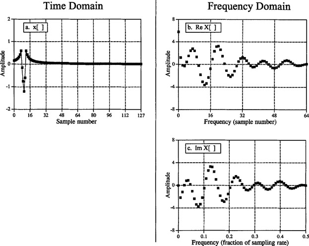
FIGURE 8-4 Example of the DFT. The DFT converts the time domain signal, x[ ], into the frequency domain signals, Re X[ ] and Im X[ ]. The horizontal axis of the frequency domain can be labeled in one of three ways: (1) as an array index that runs between 0 and N/2, (2) as a fraction of the sampling frequency, running between 0 and 0.5, (3) as a natural frequency, running between 0 and π. In the example shown here, (b) uses the first method, while (c) use the second method.
The horizontal axis of the frequency domain can be referred to in four different ways, all of which are common in DSP. In the first method, the horizontal axis is labeled from 0 to 64, corresponding to the 0 to N/2 samples in the arrays. When this labeling is used, the index for the frequency domain is an integer: for example, Re X[k] and Im X[k], where k runs from 0 to N/2 in steps of one. Programmers like this method because it is how they write code, using an index to access array locations. This notation is used in Fig. 8-4b.
In the second method, used in (c), the horizontal axis is labeled as a fraction of the sampling rate. This means that the values along the horizontal axis always run between 0 and 0.5, since discrete data can only contain frequencies between DC and one-half the sampling rate. The index used with this notation is f for frequency. The real and imaginary parts are written: Re X[f] and Im X[f], where f takes on N/2 + 1 equally spaced values between 0 and 0.5. To convert from the first notation, k, to the second notation, f, divide the horizontal axis by N. That is, f = k/N. Most of the graphs in this book use this second method, reinforcing that discrete signals only contain frequencies between 0 and 0.5 of the sampling rate.
The third style is similar to the second, except the horizontal axis is multiplied by 2π. The index used with this labeling is ω, a lower-case Greek omega. In this notation, the real and imaginary parts are written: Re X[ω] and Im X[ω)], where ω takes on N/2 + 1 equally spaced values between 0 and π. The parameter, ω, is called the natural frequency, and has the units of radians. This is based on the idea that there are 2π radians in a circle. Mathematicians like this method because it makes the equations shorter. For instance, consider how a cosine wave is written in each of these first three notations: using k: c[n] = cos(2πkn/N), using f: c[n] = cos(2πfn), and using ω: c[n] = cos((ωn).
The fourth method is to label the horizontal axis in terms of the analog frequencies used in a particular application. For instance, if the system being examined has a sampling rate of 10 kHz (i.e., 10,000 samples per second), graphs of the frequency domain would run from 0 to 5 kHz. This method has the advantage of presenting the frequency data in terms of a real world meaning. The disadvantage is that it is tied to a particular sampling rate, and is therefore not applicable to general DSP algorithm development, such as designing digital filters.
All of these four notations are used in DSP, and you need to become comfortable with converting between them. This includes both graphs and mathematical equations. To find which notation is being used, look at the independent variable and its range of values. You should find one of four notations: k (or some other integer index), running from 0 to N/2; f, running from 0 to 0.5; ω, running from 0 to π; or a frequency expressed in hertz, running from DC to one-half of an actual sampling rate.
DFT Basis Functions
The sine and cosine waves used in the DFT are commonly called the DFT basis functions. In other words, the output of the DFT is a set of numbers that represent amplitudes. The basis functions are a set of sine and cosine waves with unity amplitude. If you assign each amplitude (the frequency domain) to the proper sine or cosine wave (the basis functions), the result is a set of scaled sine and cosine waves that can be added to form the time domain signal.
The DFT basis functions are generated from the equations:
Equations for the DFT basis functions. In these equations, ck[i] and sk[ ] are the cosine and sine waves, each N points in length, running from i = 0 to N−1. The parameter, k, determines the frequency of the wave. In an N point DFT, k takes on values between 0 and N/2.

where: ck[ ] is the cosine wave for the amplitude held in Re X[k], and sk[ ] is the sine wave for the amplitude held in Im X[k]. For example, Fig. 8-5 shows some of the 17 sine and 17 cosine waves used in an N = 32 point DFT. Since these sinusoids add to form the input signal, they must be the same length as the input signal. In this case, each has 32 points running from i = 0 to 31. The parameter, k, sets the frequency of each sinusoid. In particular, c1[ ] is the cosine wave that makes one complete cycle in N points, c5[ ] is the cosine wave that makes five complete cycles in N points, etc. This is an important concept in understanding the basis functions; the frequency parameter, k, is equal to the number of complete cycles that occur over the N points of the signal.

FIGURE 8-5 DFT basis functions. A 32-point DFT has 17 discrete cosine waves and 17 discrete sine waves for its basis functions. Eight of these are shown in this figure. These are discrete signals; the continuous lines are shown in these graphs only to help the reader’s eye follow the waveforms.
Let’s look at several of these basis functions in detail. Figure (a) shows the cosine wave c0[ ]. This is a cosine wave of zero frequency, which is a constant value of one. This means that Re X[0] holds the average value of all the points in the time domain signal. In electronics, it would be said that Re X[0] holds the DC offset. The sine wave of zero frequency, s0[ ], is shown in (b), a signal composed of all zeros. Since this cannot affect the time domain signal being synthesized, the value of Im X[0] is irrelevant, and always set to zero. More about this shortly.
Figures (c) & (d) show c2[ ] & s2[ ], the sinusoids that complete two cycles in the N points. These correspond to Re X[2] & Im X[2], respectively. Likewise, (e) & (f) show c10[ ] & s10[ ], the sinusoids that complete ten cycles in the N points. These sinusoids correspond to the amplitudes held in the arrays Re X[10] & Im X[10]. The problem is, the samples in (e) and (f) no longer look like sine and cosine waves. If the continuous curves were not present in these graphs, you would have a difficult time even detecting the pattern of the waveforms. This may make you a little uneasy, but don’t worry about it. From a mathematical point of view, these samples do form discrete sinusoids, even if your eye cannot follow the pattern.
The highest frequencies in the basis functions are shown in (g) and (h). These are cN/2[ ] & sN/2[ ], or in this example, c16[ ] & s16[ ]. The discrete cosine wave alternates in value between 1 and −1, which can be interpreted as sampling a continuous sinusoid at the peaks. In contrast, the discrete sine wave contains all zeros, resulting from sampling at the zero crossings. This makes the value of Im X[N/2] the same as Im X[0], always equal to zero, and not affecting the synthesis of the time domain signal.
Here’s a puzzle: If there are N samples entering the DFT, and N+2 samples exiting, where did the extra information come from? The answer: two of the output samples contain no information, allowing the other N samples to be fully independent. As you might have guessed, the points that carry no information are Im X[0] and Im X[N/2], the samples that always have a value of zero.
Synthesis, Calculating the Inverse DFT
Pulling together everything said so far, we can write the synthesis equation:
The synthesis equation. In this relation, x[i] is the signal being synthesized, with the index, i, running from 0 to N−1.![]() and
and ![]() hold the amplitudes of the cosine and sine waves, respectively, with k running from 0 to N/2. Equation 8-3 provides the normalization to change this equation into the inverse DFT.
hold the amplitudes of the cosine and sine waves, respectively, with k running from 0 to N/2. Equation 8-3 provides the normalization to change this equation into the inverse DFT.
In words, any N-point signal, x[i], can be created by adding N/2 + 1 cosine waves and N/2 + 1 sine waves. The amplitudes of the cosine and sine waves are held in the arrays ![]() and
and ![]() , respectively. The synthesis equation multiplies these amplitudes by the basis functions to create a set of scaled sine and cosine waves. Adding the scaled sine and cosine waves produces the time-domain signal, x[i].
, respectively. The synthesis equation multiplies these amplitudes by the basis functions to create a set of scaled sine and cosine waves. Adding the scaled sine and cosine waves produces the time-domain signal, x[i].
In Eq. 8-2, the arrays are called ![]() and
and ![]() , rather than Im X[k] and Re X[k]. This is because the amplitudes needed for synthesis (called in this discussion:
, rather than Im X[k] and Re X[k]. This is because the amplitudes needed for synthesis (called in this discussion:![]() and
and ![]() ), are slightly different from the frequency domain of a signal (denoted by: Im X[k] and Re X[k]). This is the scaling factor issue we referred to earlier. Although the conversion is only a simple normalization, it is a common bug in computer programs. Look out for it! In equation form, the conversion between the two is given by:
), are slightly different from the frequency domain of a signal (denoted by: Im X[k] and Re X[k]). This is the scaling factor issue we referred to earlier. Although the conversion is only a simple normalization, it is a common bug in computer programs. Look out for it! In equation form, the conversion between the two is given by:
Conversion between the sinusoidal amplitudes and the frequency domain values. In these equations,![]() and
and ![]() hold the amplitudes of the cosine and sine waves needed for synthesis, while Re X[k] and Im X[k] hold the real and imaginary parts of the frequency domain. As usual, N is the number of points in the time domain signal, and k is an index that runs from 0 to N/2.
hold the amplitudes of the cosine and sine waves needed for synthesis, while Re X[k] and Im X[k] hold the real and imaginary parts of the frequency domain. As usual, N is the number of points in the time domain signal, and k is an index that runs from 0 to N/2.

Suppose you are given a frequency domain representation, and asked to synthesize the corresponding time domain signal. To start, you must find the amplitudes of the sine and cosine waves. In other words, given ![]() and
and ![]() , you must find
, you must find ![]() and
and ![]() . Equation 8-3 shows this in a mathematical form. To do this in a computer program, three actions must be taken. First, divide all the values in the frequency domain by N/2. Second, change the sign of all the imaginary values. Third, divide the first and last samples in the real part, Re X[0] and Re X[N/2], by two. This provides the amplitudes needed for the synthesis described by Eq. 8-2. Taken together, Eqs. 8-2 and 8-3 define the inverse DFT.
. Equation 8-3 shows this in a mathematical form. To do this in a computer program, three actions must be taken. First, divide all the values in the frequency domain by N/2. Second, change the sign of all the imaginary values. Third, divide the first and last samples in the real part, Re X[0] and Re X[N/2], by two. This provides the amplitudes needed for the synthesis described by Eq. 8-2. Taken together, Eqs. 8-2 and 8-3 define the inverse DFT.
The entire inverse DFT is shown in the computer program listed in Table 8-1. There are two ways that the synthesis (Eq. 8-2) can be programmed, and both are shown. In the first method, each of the scaled sinusoids are generated one at a time and added to an accumulation array, which ends up becoming the time domain signal. In the second method, each sample in the time domain signal is calculated one at a time, as the sum of all the corresponding samples in the cosine and sine waves. Both methods produce the same result. The difference between these two programs is very minor; the inner and outer loops are swapped during the synthesis.
TABLE 8-1

Figure 8-6 illustrates the operation of the inverse DFT, and the slight differences between the frequency domain and the amplitudes needed for synthesis. Figure 8-6a is an example signal we wish to synthesize, an impulse at sample zero with an amplitude of 32. Figure 8-6b shows the frequency domain representation of this signal. The real part of the frequency domain is a constant value of 32. The imaginary part (not shown) is composed of all zeros. As discussed in the next chapter, this is an important DFT pair: an impulse in the time domain corresponds to a constant value in the frequency domain. For now, the important point is that (b) is the DFT of (a), and (a) is the Inverse DFT of (b).

FIGURE 8-6 Example of the inverse DFT. Figure (a) shows an example time domain signal, an impulse at sample zero with an amplitude of 32. Figure (b) shows the real part of the frequency domain of this signal, a constant value of 32. The imaginary part of the frequency domain (not shown) is composed of all zeros. Figure(c) shows the amplitudes of the cosine waves needed to reconstruct (a) using Eq. 8-2. The values in (c) are found from (b) by using Eq. 8-3.
Equation 8-3 is used to convert the frequency domain signal, (b), into the amplitudes of the cosine waves, (c). As shown, all of the cosine waves have an amplitude of two, except for samples 0 and 16, which have a value of one. The amplitudes of the sine waves are not shown in this example because they have a value of zero, and therefore provide no contribution. The synthesis equation, Eq. 8-2, is then used to convert the amplitudes of the cosine waves, (b), into the time domain signal, (a).
This describes how the frequency domain is different from the sinusoidal amplitudes, but it doesn’t explain why it is different. The difference occurs because the frequency domain is defined as a spectral density. Figure 8-7 shows how this works. The example in this figure is the real part of the frequency domain of a 32-point signal. As you should expect, the samples run from 0 to 16, representing 17 frequencies equally spaced between 0 and 1/2 of the sampling rate. Spectral density describes how much signal (amplitude) is present per unit of bandwidth. To convert the sinusoidal amplitudes into a spectral density, divide each amplitude by the bandwidth represented by each amplitude. This brings up the next issue: how do we determine the bandwidth of each of the discrete frequencies in the frequency domain?

FIGURE 8-7 The bandwidth of frequency domain samples. Each sample in the frequency domain can be thought of as being contained in a frequency band of width 2/N, expressed as a fraction of the total bandwidth. An exception to this is the first and last samples, which have a bandwidth only one-half this wide, 1/N.
As shown in the figure, the bandwidth can be defined by drawing dividing lines between the samples. For instance, sample number 5 occurs in the band between 4.5 and 5.5; sample number 6 occurs in the band between 5.5 and 6.5, etc. Expressed as a fraction of the total bandwidth (i.e., N/2), the bandwidth of each sample is 2/N. An exception to this is the samples on each end, which have one-half of this bandwidth, 1/N. This accounts for the 2/N scaling factor between the sinusoidal amplitudes and frequency domain, as well as the additional factor of two needed for the first and last samples.
Why the negation of the imaginary part? This is done solely to make the real DFT consistent with its big brother, the complex DFT. In Chapter 29 we will show that it is necessary to make the mathematics of the complex DFT work. When dealing only with the real DFT, many authors do not include this negation. For that matter, many authors do not even include the 2/N scaling factor. Be prepared to find both of these missing in some discussions. They are included here for a tremendously important reason: The most efficient way to calculate the DFT is through the fast Fourier transform (FFT) algorithm, presented in Chapter 12. The FFT generates a frequency domain defined according to Eq. 8-2 and 8-3. If you start messing with these normalization factors, your programs containing the FFT are not going to work as expected.
Analysis, Calculating the DFT
The DFT can be calculated in three completely different ways. First, the problem can be approached as a set of simultaneous equations. This method is useful for understanding the DFT, but it is too inefficient to be of practical use. The second method brings in an idea from the last chapter: correlation. This is based on detecting a known waveform in another signal. The third method, called the fast Fourier transform (FFT), is an ingenious algorithm that decomposes a DFT with N points, into N DFTs each with a single point. The FFT is typically hundreds of times faster than the other methods. The first two methods are discussed here, while the FFT is the topic of Chapter 12. It is important to remember that all three of these methods produce an identical output. Which should you use? In actual practice, correlation is the preferred technique if the DFT has less than about 32 points; otherwise the FFT is used.
DFT by Simultaneous Equations
Think about the DFT calculation in the following way. You are given N values from the time domain, and asked to calculate the N values of the frequency domain (ignoring the two frequency domain values that you know must be zero). Basic algebra provides the answer: to solve for N unknowns, you must be able to write N linearly independent equations. To do this, take the first sample from each sinusoid and add them together. The sum must be equal to the first sample in the time domain signal, thus providing the first equation. Likewise, an equation can be written for each of the remaining points in the time domain signal, resulting in the required N equations. The solution can then be found by using established methods for solving simultaneous equations, such as Gauss Elimination. Unfortunately, this method requires a tremendous number of calculations, and is virtually never used in DSP. However, it is important for another reason, it shows why it is possible to decompose a signal into sinusoids, how many sinusoids are needed, and that the basis functions must be linearly independent (more about this shortly).
DFT by Correlation
Let’s move on to a better way, the standard way of calculating the DFT. An example will show how this method works. Suppose we are trying to calculate the DFT of a 64-point signal. This means we need to calculate the 33 points in the real part, and the 33 points in the imaginary part of the frequency domain. In this example we will only show how to calculate a single sample, Im X[3], i.e., the amplitude of the sine wave that makes three complete cycles between point 0 and point 63. All of the other frequency domain values are calculated in a similar manner.
Figure 8-8 illustrates using correlation to calculate Im X[3]. Figures (a) and (b) show two example time domain signals, called: x1[ ] and x2[ ], respectively. The first signal, x1[ ], is composed of nothing but a sine wave that makes three cycles between points 0 and 63. In contrast, x2[ ] is composed of several sine and cosine waves, none of which make three cycles between points 0 and 63. These two signals illustrate what the algorithm for calculating Im X[3] must do. When fed x1[ ], the algorithm must produce a value of 32, the amplitude of the sine wave present in the signal (modified by the scaling factors of Eq. 8-3). In comparison, when the algorithm is fed the other signal, x2[ ], a value of zero must be produced, indicating that this particular sine wave is not present in this signal.

FIGURE 8-8 Two example signals, (a) and (b), are analyzed for containing the specific basis function shown in (c) and (d). Figures (e) and (f) show the result of multiplying each example signal by the basis function. Figure (e) has an average of 0.5, indicating that x1[ ] contains the basis function with an amplitude of 1.0. Conversely, (f) has a zero average, indicating that x2[ ] does not contain the basis function.
The concept of correlation was introduced in Chapter 7. As you recall, to detect a known waveform contained in another signal, multiply the two signals and add all the points in the resulting signal. The single number that results from this procedure is a measure of how similar the two signals are. Figure 8-8 illustrates this approach. Figures (c) and (d) both display the signal we are looking for, a sine wave that makes 3 cycles between samples 0 and 63. Figure (e) shows the result of multiplying (a) and (c). Likewise, (f) shows the result of multiplying (b) and (d). The sum of all the points in (e) is 32, while the sum of all the points in (f) is zero, showing we have found the desired algorithm.
The other samples in the frequency domain are calculated in the same way. This procedure is formalized in the analysis equation, the mathematical way to calculate the frequency domain from the time domain:
The analysis equations for calculating the DFT. In these equations, x[i] is the time domain signal being analyzed, and Re X[k] & Im X[k] are the frequency domain signals being calculated. The index i runs from 0 to N−1, while the index k runs from 0 to N/2.

In words, each sample in the frequency domain is found by multiplying the time domain signal by the sine or cosine wave being looked for, and adding the resulting points. If someone asks you what you are doing, say with confidence: “I am correlating the input signal with each basis function.” Table 8-2 shows a computer program for calculating the DFT in this way.
TABLE 8-2

The analysis equation does not require special handling of the first and last points, as did the synthesis equation. There is, however, a negative sign in the imaginary part in Eq. 8-4. Just as before, this negative sign makes the real DFT consistent with the complex DFT, and is not always included.
In order for this correlation algorithm to work, the basis functions must have an interesting property: each of them must be completely uncorrelated with all of the others. This means that if you multiply any two of the basis functions, the sum of the resulting points will be equal to zero. Basis functions that have this property are called orthogonal. Many other orthogonal basis functions exist, including: square waves, triangle waves, impulses, etc. Signals can be decomposed into these other orthogonal basis functions using correlation, just as done here with sinusoids. This is not to suggest that this is useful, only that it is possible.
As previously shown in Table 8-1, the inverse DFT has two ways to be implemented in a computer program. This difference involves swapping the inner and outer loops during the synthesis. While this does not change the output of the program, it makes a difference in how you view what is being done. The DFT program in Table 8-2 can also be changed in this fashion, by swapping the inner and outer loops in lines 310 to 380. Just as before, the output of the program is the same, but the way you think about the calculation is different. (These two different ways of viewing the DFT and inverse DFT could be described as “input side” and “output side” algorithms, just as for convolution).
As the program in Table 8-2 is written, it describes how an individual sample in the frequency domain is affected by all of the samples in the time domain. That is, the program calculates each of the values in the frequency domain in succession, not as a group. When the inner and outer loops are exchanged, the program loops through each sample in the time domain, calculating the contribution of that point to the frequency domain. The overall frequency domain is found by adding the contributions from the individual time domain points. This brings up our next question: what kind of contribution does an individual sample in the time domain provide to the frequency domain? The answer is contained in an interesting aspect of Fourier analysis called duality.
Duality
The synthesis and analysis equations (Eqs. 8-2 and 8-4) are strikingly similar. To move from one domain to the other, the known values are multiplied by the basis functions, and the resulting products added. The fact that the DFT and the inverse DFT use this same mathematical approach is really quite remarkable, considering the totally different way we arrived at the two procedures. In fact, the only significant difference between the two equations is a result of the time domain being one signal of N points, while the frequency domain is two signals of N/2 + 1 points. As discussed in later chapters, the complex DFT expresses both the time and the frequency domains as complex signals of N points each. This makes the two domains completely symmetrical, and the equations for moving between them virtually identical.
This symmetry between the time and frequency domains is called duality, and gives rise to many interesting properties. For example, a single point in the frequency domain corresponds to a sinusoid in the time domain. By duality, the inverse is also true, a single point in the time domain corresponds to a sinusoid in the frequency domain. As another example, convolution in the time domain corresponds to multiplication in the frequency domain. By duality, the reverse is also true: convolution in the frequency domain corresponds to multiplication in the time domain. These and other duality relationships are discussed in more detail in Chapters 10 and 11.
Polar Notation
As it has been described so far, the frequency domain is a group of amplitudes of cosine and sine waves (with slight scaling modifications). This is called rectangular notation. Alternatively, the frequency domain can be expressed in polar form. In this notation, Re X[ ] & Im X[ ] are replaced with two other arrays, called the Magnitude of X[ ], written in equations as: Mag X[ ], and the Phase of X[ ], written as: Phase X[ ]. The magnitude and phase are a pair-for-pair replacement for the real and imaginary parts. For example, Mag X[0] and Phase X[0] are calculated using only Re X[0] and Im X[0]. Likewise, Mag X[14] and Phase X[14] are calculated using only Re X[14] and Im X[14], and so forth. To understand the conversion, consider what happens when you add a cosine wave and a sine wave of the same frequency. The result is a cosine wave of the same frequency, but with a new amplitude and a new phase shift. In equation form, the two representations are related:
The addition of a cosine and sine wave results in a cosine wave with a different amplitude and phase shift. The information contained in A & B is transferred to two other variables, M and θ.
The important point is that no information is lost in this process; given one representation you can calculate the other. In other words, the information contained in the amplitudes A and B, is also contained in the variables M and θ. Although this equation involves sine and cosine waves, it follows the same conversion equations as do simple vectors. Figure 8-9 shows the analogous vector representation of how the two variables, A and B, can be viewed in a rectangular coordinate system, while M and θ are parameters in polar coordinates.

FIGURE 8-9 Rectangular-to-polar conversion. The addition of a cosine wave and a sine wave (of the same frequency) follows the same mathematics as the addition of simple vectors.
In polar notation, Mag X[ ] holds the amplitude of the cosine wave (M in Eq. 8-5 and Fig. 8-9), while Phase X[ ] holds the phase angle of the cosine wave (θ in Eq. 8-5 and Fig. 8-9). The following equations convert the frequency domain from rectangular to polar notation, and vice versa:
Rectangular-to-polar conversion. The rectangular representation of the frequency domain, Re X[k] and Im X[k], is changed into the polar form, Mag X[k] and Phase X[k].

Polar-to-rectangular conversion. The two arrays, Mag X[k] and Phase X[k], are converted into Re X[k] and Im X[k].

Rectangular and polar notation allows you to think of the DFT in two different ways. With rectangular notation, the DFT decomposes an N-point signal into N/2 + 1 cosine waves and N/2 + 1 sine waves, each with a specified amplitude. In polar notation, the DFT decomposes an N-point signal into N/2 + 1 cosine waves, each with a specified amplitude (called the magnitude) and phase shift. Why does polar notation use cosine waves instead of sine waves? Sine waves cannot represent the DC component of a signal, since a sine wave of zero frequency is composed of all zeros (see Figs. 8-5 a and b).
Even though the polar and rectangular representations contain exactly the same information, there are many instances where one is easier to use than the other. For example, Fig. 8-10 shows a frequency domain signal in both rectangular and polar form. Warning: Don’t try to understand the shape of the real and imaginary parts; your head will explode! In comparison, the polar curves are straightforward: only frequencies below about 0.25 are present, and the phase shift is approximately proportional to the frequency. This is the frequency response of a low-pass filter.

FIGURE 8-10 Example of rectangular and polar frequency domains. This example shows a frequency domain expressed in both rectangular and polar notation. As in this case, polar notation usually provides human observers with a better understanding of the characteristics of the signal. In comparison, the rectangular form is almost always used when math computations are required. Pay special notice to the fact that the first and last samples in the phase must be zero, just as they are in the imaginary part.
When should you use rectangular notation and when should you use polar? Rectangular notation is usually the best choice for calculations, such as in equations and computer programs. In comparison, graphs are almost always in polar form. As shown by the previous example, it is nearly impossible for humans to understand the characteristics of a frequency domain signal by looking at the real and imaginary parts. In a typical program, the frequency domain signals are kept in rectangular notation until an observer needs to look at them, at which time a rectangular-to-polar conversion is done.
Why is it easier to understand the frequency domain in polar notation? This question goes to the heart of why decomposing a signal into sinusoids is useful. Recall the property of sinusoidal fidelity from Chapter 5: if a sinusoid enters a linear system, the output will also be a sinusoid, and at exactly the same frequency as the input. Only the amplitude and phase can change. Polar notation directly represents signals in terms of the amplitude and phase of the component cosine waves. In turn, systems can be represented by how they modify the amplitude and phase of each of these cosine waves.
Now consider what happens if rectangular notation is used with this scenario. A mixture of cosine and sine waves enter the linear system, resulting in a mixture of cosine and sine waves leaving the system. The problem is, a cosine wave on the input may result in both cosine and sine waves on the output. Likewise, a sine wave on the input can result in both cosine and sine waves on the output. While these cross-terms can be straightened out, the overall method doesn’t match with why we wanted to use sinusoids in the first place.
Polar Nuisances
There are many nuisances associated with using polar notation. None of these are overwhelming, just really annoying! Table 8-3 shows a computer program for converting between rectangular and polar notation, and provides solutions for some of these pests.
TABLE 8-3

Nuisance 1: Radians vs. Degrees
It is possible to express the phase in either degrees or radians. When expressed in degrees, the values in the phase signal are between −180 and 180. Using radians, each of the values will be between −π and π—that is, between −3.141592 to 3.141592. Most computer languages require the use of radians for their trigonometric functions, such as cosine, sine, arctangent, etc. It can be irritating to work with these long decimal numbers, and difficult to interpret the data you receive. For example, if you want to introduce a 90-degree phase shift into a signal, you need to add 1.570796 to the phase. While it isn’t going to kill you to type this into your program, it does become tiresome. The best way to handle this problem is to define the constant, PI = 3.141592, at the beginning of your program. A 90-degree phase shift can then be written as PI/2. Degrees and radians are both widely used in DSP and you need to become comfortable with both.
Nuisance 2: Divide by zero error
When converting from rectangular to polar notation, it is very common to find frequencies where the real part is zero and the imaginary part is some nonzero value. This simply means that the phase is exactly 90 or −90 degrees. Try to tell your computer this! When your program tries to calculate the phase from: Phase X[k] = arctan(Im X[k]/Re X[k]), a divide by zero error occurs. Even if the program execution doesn’t halt, the phase you obtain for this frequency won’t be correct. To avoid this problem, the real part must be tested for being zero before the division. If it is zero, the imaginary part must be tested for being positive or negative, to determine whether to set the phase to π/2 or −π/2, respectively. Lastly, the division needs to be bypassed. Nothing difficult in all these steps, just the potential for aggravation. An alternative way to handle this problem is shown in line 250 of Table 8-3. If the real part is zero, change it to a negligibly small number to keep the math processor happy during the division.
Nuisance 3: Incorrect arctan
Consider a frequency domain sample where Re X[k] = 1 and Im X[k] = 1. Equation 8-6 provides the corresponding polar values of Mag X[k] = 1.414 and Phase X[k] = 45°. Now consider another sample where Re X[k] = −1 and Im X[k] = −1. Again, Eq. 8-6 provides the values of Mag X[k] = 1.414 and Phase X[k] = 45°. The problem is, the phase is wrong! It should be −135°. This error occurs whenever the real part is negative. This problem can be corrected by testing the real and imaginary parts after the phase has been calculated. If both the real and imaginary parts are negative, subtract 180° (or π radians) from the calculated phase. If the real part is negative and the imaginary part is positive, add 180° (or π radians). Lines 340 and 350 of the program in Table 8-3 show how this is done. If you fail to catch this problem, the calculated value of the phase will only run between −π/2 and π/2, rather than between −π and π. Drill this into your mind. If you see the phase only extending to ±1.5708, you have forgotten to correct the ambiguity in the arctangent calculation.
Nuisance 4: Phase of very small magnitudes
Imagine the following scenario. You are grinding away at some DSP task, and suddenly notice that part of the phase doesn’t look right. It might be noisy, jumping all over, or just plain wrong. After spending the next hour looking through hundreds of lines of computer code, you find the answer. The corresponding values in the magnitude are so small that they are buried in round-off noise. If the magnitude is negligibly small, the phase doesn’t have any meaning, and can assume unusual values. An example of this is shown in Fig. 8-11. It is usually obvious when an amplitude signal is lost in noise; the values are so small that you are forced to suspect that the values are meaningless. The phase is different. When a polar signal is contaminated with noise, the values in the phase are random numbers between −π and π. Unfortunately, this often looks like a real signal, rather than the nonsense it really is.

Nuisance 5: 2π ambiguity of the phase
Look again at Fig. 8-10d, and notice the several discontinuities in the data. Every time a point looks as if it is going to dip below −3.14592, it snaps back to 3.141592. This is a result of the periodic nature of sinusoids. For example, a phase shift of θ is exactly the same as a phase shift of θ + 2π, θ + 4π, θ + 6π, etc. Any sinusoid is unchanged when you add an integer multiple of 2π to the phase. The apparent discontinuities in the signal are a result of the computer algorithm picking its favorite choice from an infinite number of equivalent possibilities. The smallest possible value is always chosen, keeping the phase between −π and π.
It is often easier to understand the phase if it does not have these discontinuities, even if it means that the phase extends above π, or below −π. This is called unwrapping the phase, and an example is shown in Fig. 8-12. As shown by the program in Table 8-4, a multiple of 2π is added or subtracted from each value of the phase. The exact value is determined by an algorithm that minimizes the difference between adjacent samples.
TABLE 8-4


FIGURE 8-12 Example of phase unwrapping. The top curve shows a typical phase signal obtained from a rectangular-to-polar conversion routine. Each value in the signal must be between −π and π (i.e., −3.14159 and 3.14159). As shown in the lower curve, the phase can be unwrapped by adding or subtracting integer multiplies of 2π from each sample, where the integer is chosen to minimize the discontinuities between points.
Nuisance 6: The magnitude is always positive (π ambiguity of the phase)
Figure 8-13 shows a frequency domain signal in rectangular and polar form. The real part is smooth and quite easy to understand, while the imaginary part is entirely zero. In comparison, the polar signals contain abrupt discontinuities and sharp corners. This is because the magnitude must always be positive, by definition. Whenever the real part dips below zero, the magnitude remains positive by changing the phase by π (or −π, which is the same thing). While this is not a problem for the mathematics, the irregular curves can be difficult to interpret.

FIGURE 8-13 Example signals in rectangular and polar form. Since the magnitude must always be positive (by definition), the magnitude and phase may contain abrupt discontinuities and sharp corners. Figure (d) also shows another nuisance: random noise can cause the phase to rapidly oscillate between π or −π.
One solution is to allow the magnitude to have negative values. In the example of Fig. 8-13, this would make the magnitude appear the same as the real part, while the phase would be entirely zero. There is nothing wrong with this if it helps your understanding. Just be careful not to call a signal with negative values the “magnitude” since this violates its formal definition. In this book we use the weasel words: unwrapped magnitude to indicate a “magnitude” that is allowed to have negative values.
Nuisance 7: Spikes between π and −π
Since π and −π represent the same phase shift, round-off noise can cause adjacent points in the phase to rapidly switch between the two values. As shown in Fig. 8-13d, this can produce sharp breaks and spikes in an otherwise smooth curve. Don’t be fooled; the phase isn’t really this discontinuous.