3

Digital Filters

We use digital filters [1] on many occasions without our knowledge. The main reason for this is that any sequence of numbers if multiplied¹ and added constitutes a simple linear filter. The temperature of a bulb follows a similar law but with some more modifications. Computing compound interest has a similar structure.

Such filters are nothing but a difference equation with or without feedback. For a software engineer it is a piece of code; for a hardware engineer it is an assembly of shift registers, adders, multipliers and control logic.

Converting a difference equation to a program is fairly simple and routine. The key step is to choose the coefficients of the difference equation so they suit your purpose. There are many methods available in the published literature [1, 2] for obtaining the coefficients in these difference equations. There are also many powerful software packages² available to assist the designer in the implementation.

There is another class of design approach required in many practical situations, where we need to obtain the filter coefficients given the measured impulse response of the filter (h_k), or given an input (u_k) and an output sequence (y_k), or given the amplitude and phase response of the filter. Problems of this type are known as inverse problems. For a difference equation, obtaining the output corresponding to a given input is relatively easy and is known as the forward problem.

3.1 How to Specify a Filter

Conventionally filters are specified in the frequency domain. For a better understanding, consider the filter in Figure 3.1. There are three important parameters that often need to be specified when designing a filter. Conventionally, slope or roll-off is defined in dB/decade or dB/octave.

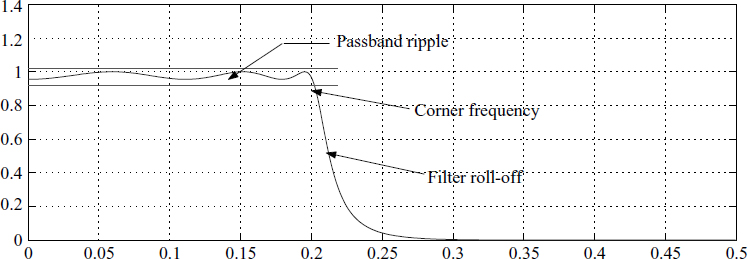
Figure 3.1 Filter specifications

The unit dB/octave is from music and acoustics. The unit dB/decade is from control engineering; it is slowly becoming more prevalent in filter design. Most of the programs available demand the order of the filter. A simple rule of thumb is if N is the order of the system, then the corresponding slope at the cut-off frequency is 20N dB/decade. A quick reference to Figure 3.1 shows a typical filter specification in the frequency domain. We specify the filter using

• Passband or stopband ripple in dB
• Corner frequency or cut-off frequency
• Roll-off defined in dB/decade

3.2 Moving-Average Filters

Moving-average (MA) filters are the simplest filters and can be well understood without much difficulty. The basic reason is that there is no feedback in these filters. The advantage is that they are always stable and easy to implement. On the other hand, filters with feedback elements but no feedforward elements are called autoregressive (AR) filters. Here are some examples.

3.2.1 Area under a Curve

The most common MA filters are used for finding the area under a portion of a curve by the trapezium rule or Simpson's rule, represented as

where {u_k} is the input and{u_k} the output. The objective of these two filters is to find the area between the points by finding out the weighted mean (u_k) of the ordinates.

3.2.2 Mean of a Given Sequence

Finding the mean of a given sequence is another application for an MA filter. However, the mean of a sequence of length N can also be found recursively, resulting in an AR filter. We derived this in (1.41). It is given as

Another filter commonly used is an exponential weighted-averaging filter with similar structure (also known as a fading filter); it is given as

This filter is used for finding out the mean when distant values are of no significance. In fact there is no difference between the filters in (3.4) and (3.5); it is only the contexts that are different. The solution for (3.5) is of the form y_k = (Aλ^k) ⊗ u_k, where A is a constant that can be obtained from the initial conditions and ⊗ represents convolution. The general choice of the coefficient is 0.8 ≤ λ ≤ 0.95.

3.2.3 Mean over a Fixed Number of Samples

The filter in (3.4) finds the mean of a given set of samples. However, on many occasions, we need to find continuously the mean over a fixed number of samples. This can be done using the filter in (3.5), but then the far samples are weighted low compared to the near samples.

Consider the case when we need to compute the mean (μ_k) over n = k to n = k + N − 1 for the given time series u_k as shown in Figure 3.2. This is mathematically given as

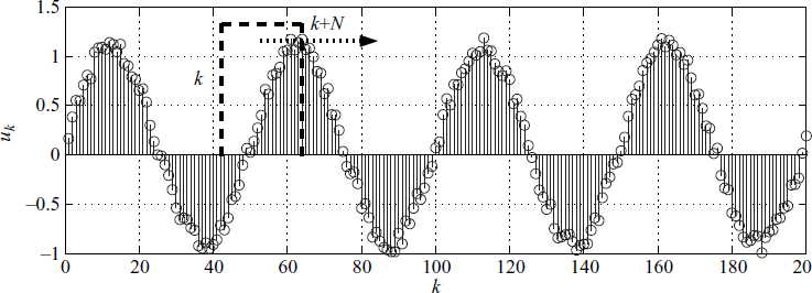
Figure 3.2 Rectangular moving filter

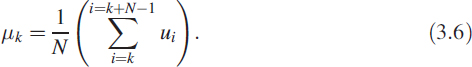
To arrive at the recursive form similar to (3.4), we rewrite μ_k+1 as

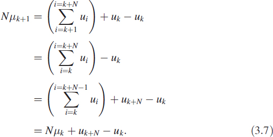
Equation (3.7) can be written as

The moving mean μ_k is obtained by passing the signal ge_k through an integrator (3.8). This integrator can be written in operator notation or as a transfer function (TF) model:

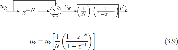
The filter in (3.9) has feedback and feedforward elements and is called an autoregressive moving average (ARMA) filter. This filter is stable in spite of a pole on the unit circle due to the pole–zero cancellation at z = 1.

3.2.4 Linear Phase Filters

Consider a narrowband filter (NBF) given by (3.17). Let the impulse response of this IIR filter be h_k. We truncate the infinite series h_k and use these values to generate the coefficients of an MA filter in a specific way, given by

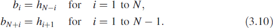
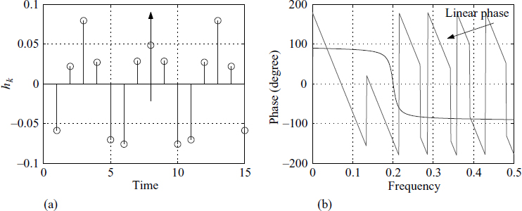
Figure 3.3 Coefficients of a moving-average filter

The coefficient vector b, comprising the b_i stacked together, is of dimension 2N − 1; it is shown in Figure 3.3(a). Notice that the coefficients are symmetric; we have drawn an arrow at the symmetric point.

From the theory of polynomials, we recollect that such a symmetric property produces a linear phase characteristic. The same is shown in Figure 3.3(b), which shows the linear phase of the MA filter. In the same figure, we see the corresponding non-linear phase of the original (parent) IIR narrowband filter. The choice of these coefficients is deliberate and is intended to describe the linear phase property. In addition, we demonstrate conversion of an IIR filter to an MA filter using the truncated impulse response of the IIR filter.

Figure 3.4 shows the frequency response of the IIR filter and the MA filter (truncated IIR). The performance of the IIR filter is far superior to the performance of the MA filter. Computationally, an IIR filter needs less resources, but stability and phase are the compromises. In addition, a careful examination reveals a compromise in the filter's skirt sharpness and its sidelobe levels are high.

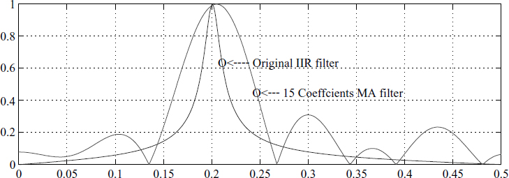
Figure 3.4 Moving-average filter

3.2.5 MA Filter with Complex Coefficients

There is another important breed of MA filters based on the concept of super-heterodyning. This consists of a local oscillator, a mixer, and a filter. The signal x(t) is multiplied with a local oscillator e^−j2πft and passed through an integral or lowpass filter. Mathematically,³ it is given by

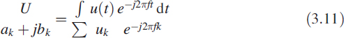
Equation (3.11) depicts a mapping from continuous to discrete. This means that we beat the given signal u_k with an oscillator and pass the result through a summation. This results in a pair of MA filters:

Figure 3.5 is an implementation of (3.12) with non-linear devices such as multipliers.

Figure 3.5 Heterodyning

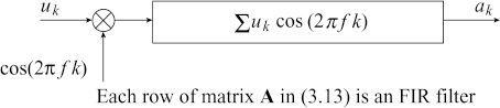
When we sweep the oscillator to generate a set of rows resulting in a pair of matrices, one for real (in-phase or cosine) and one for imaginary (quadrature or sine), we can also observe the output as Fourier series coefficients.

Instead of using an infinite sine wave, we can sample the sine wave to generate the coefficients of the MA filter. The filter characteristics depend on the number of coefficients and how many samples are taken per cycle. Consider a matrix A with each row containing the coefficients of an MA filter.

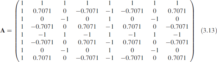
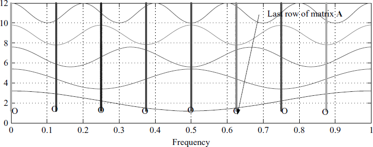
Figure 3.6 How to understand matrix A in (3.12)

We get a better insight into the entries of the matrix A by looking at Figure 3.6. Look back and forth between Figures 3.6 and 3.5 and glance at the matrix (3.13). This will help you understand what is going on. A close look at Figure 3.6 shows that cosine waves are sampled at 8 places simultaneously, leading to various rows in the matrix A.

Note that each row represents an oscillator. The choice of the coefficients is not arbitrary but has a definite pattern. The last row of A consists of 8 samples of one full cycle of a cosine wave. We have two matrices, one for the real part and one for the complex part. The entries of each row are sampled cosine values or sine values. The given input is passed through these two filters and this creates two orthogonal outputs. It is not necessary to have a square matrix, but there is a computational advantage in choosing a square matrix of order 2ⁿ.

All these filters have linear phase characteristics. Consider the row vector a_i, the ith row of the matrix A. The output is an MA process.

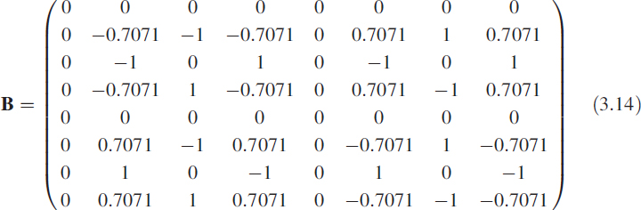
The matrix B in (3.14) corresponds to the imaginary part of the coefficients; the rest of the explanation is the same as for A. Figure 3.7 shows the in-phase and quadrature results for matrices A and B.

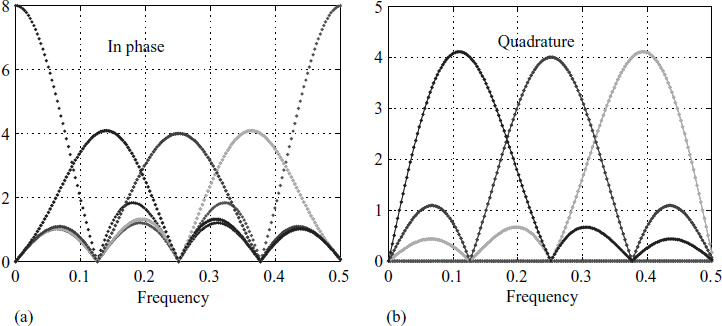
Figure 3.7 Bank of filters in matrices A and B in (3.13) and (3.14)

3.3 Infinite Sequence Generation

In many applications, we need to generate an infinite sequence of numbers for testing or as part of the system modelling. Here are a few examples.

3.3.1 Digital Counter

In many programing applications we use counters. Such counters are obtained by using an integrator with an input as a Kronecker delta function given by δ_k = 1 for only k = 0, and the input–output relation

Quite often this model is used in real-time simulations for generating a ramp.

3.3.2 Noise Sequence

The primary source is a uniformly distributed noise (UDN), which can be generated by a linear congruential generator (LCG), explained in Section 2.4.1. Figure 3.8

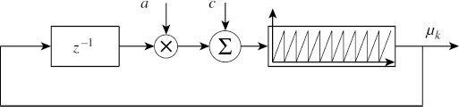
Figure 3.8 Non-linear infinite sequence generator

shows the relation of an LCG given as μ_k = (aμ_k−1 + c) mod m, where the constants a and c can be chosen to suit the purpose. This is an example of a filter with a non-linear element in the feedback loop.

3.3.3 Numerically Controlled Oscillator

Consider this statement:

Translated into an equation, this is

Equation (3.16) results in the infinite sequence of Figure 3.9; it is a sinusoidal wave with a normalised frequency . The infinite sequence {y_k} generated by the 3-tuple {1.8,1,0} illustrates a method for data compression. In addition, by varying only the coefficient of y_k−1, we can control the frequency; this is an important result used in the implementation of a numerically controlled oscillator (NCO). Consider a simple pendulum oscillating. If we watch this using a stroboscope, the angle seen at the time of flash is θ_k = θ_k−1 − θ_k−2, where is a constant that depends on the flash frequency, the length of the pendulum, and the acceleration due to gravity at that place.

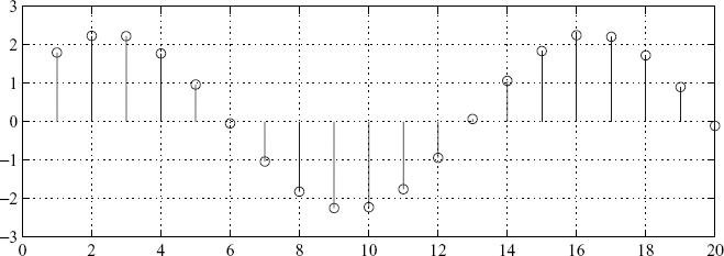
Figure 3.9 Numerically controlled oscillator

3.4 Unity-Gain Narrowband Filter

One of the most popular filters is the narrowband filter (NBF). It is used in every domain of filter design. All filter designs of higher order use cascades of NBFs having different parameters. In superheterodyning receivers, the NBF is used immediately after the mixer stage. It is also very common in notch filters. In such filters there is a need to have unity gain around the peak response and zero gains at DC and at the Nyquist frequency, resulting in an input–output relation

where p = 2 cos θ, with θ = 2πf and g = (1 — r²)/2. We note that −2 ≤ p ≤ 2. For stability, we need 0 < r < 1. The frequency response of the NBF is given in Figure 3.10. It has gain zero at 0 and 0.5 due to the two zeros present at these places, with a = [1 − rp r²] and b = g[10 − 1]. Equation (3.17), for an NBF, becomes an NCO equation when we substitute r = 1.

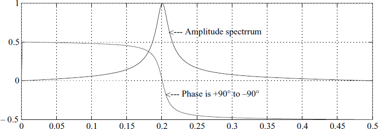
Figure 3.10 Bandpass filter with r = 0.95 and f = 0.2

3.5 All-Pass Filter

Many times we need to control the phase of the sequence or need to interpolate the values of a given sequence. This is best done by filters of first order or second order. In the first-order filter, we need to remember just one old value; in the second-order filter, we need to remember two old values. A typical first-order all-pass filter (APF) has the structure

The second-order filter is

These two all-pass filters represent a real-pole filter and a complex-pole filter, respectively. When we have complex poles, the roots bear a reciprocal conjugate relation. This can be best understood by writing (3.19) in operator notation:

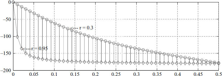
Figure 3.11 Phase of a first-order all-pass filter

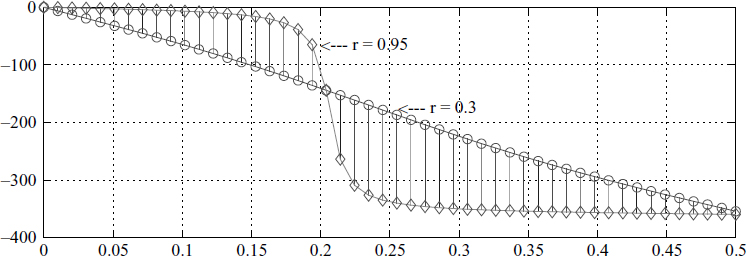
Figure 3.12 Phase of a second-order all-pass filter

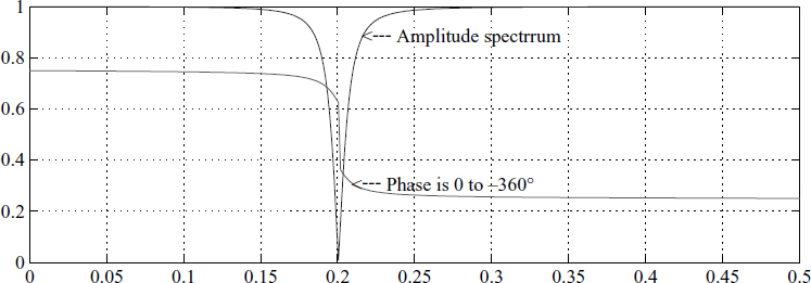
The phase shown in Figure 3.11 is for a real-pole filter. Notice the sensitivity of r in controlling phase, and notice that between 50 samples/cycle and 4 samples/cycle the filter is very effective at controlling the phase. Figure 3.12 shows the phase of a complex all-pass filter and its sensitivity to the radial pole position.

3.5.1 Interpolation of Data Using an APF

A typical data acquisition system with more than one signal has the structure given in Figure 3.13. This structure is chosen for economy and to make best use of the A/D converter's bandwidth.

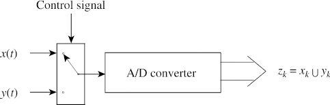
Figure 3.13 Phase shift in the data acquisition

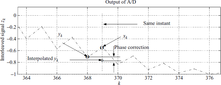
Figure 3.14 Correcting the phase shift

The signals x(t) or⁴ y(t) are passed through an analogue multiplexer, with the help of a control signal. The digitised signals x_k and y_k are interleaved to yield z_k = x_k ∪ y_k and passed to the processor for further processing in the digital domain. Ideally, the requirement is to sample the signals at the same time. However, to reduce the amount of hardware, we decide to use only a single A/D converter. Refer to Figure 3.14; what we need is the interpolated value of y_k = ŷ_k corresponding to x_k. It implies that we should not take the two sequences {x_k} and {y_k} for further processing, but the sequences {x_k} and {ŷ_k}. And this implies three things:

1. The interleaved sequence z_k needs to be separated as x_k and y_k.
2. We reconstruct the sequence ŷ_k from y_k by passing through an APF.
3. We use this pair of sequences {x_k} and {ŷ_k} as if they are sampled simultaneously.

Obtaining the sequence {ŷ_k} is known as phase correction and is shown in Figure 3.14. This should be done for the entire sequence with linear phase characteristics. It is typically done using an APF.

3.5.2 Delay Estimation Using an APF

We demonstrate an adaptive APF for estimating the delay between two sinusoidal signals. An APF has a flat frequency response and a variable phase response. We best use this principle by varying the pole and zero positions. Consider two omnidirectional antenna elements spaced at a distance d ≤ λ/2 to avoid the grating lobe phenomenon (similar to the aliasing problem in the time domain). Estimating the value of φ is important to find out the direction of an emitter producing narrowband signals.

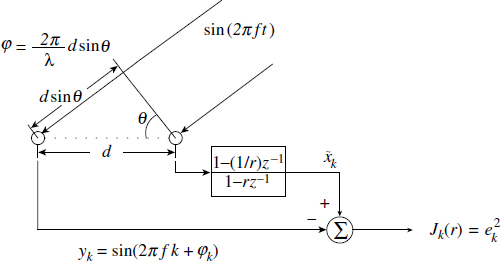
Figure 3.15 Delay estimation using an all-pass filter

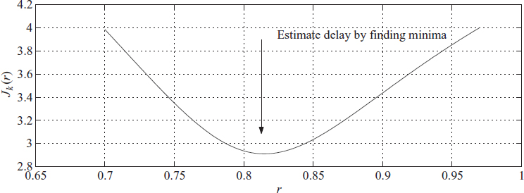
Figure 3.16 Varying the parameter r for delay estimation

The signal received at the first element after digitisation is x_k = sin(2πfk) and the signal at the second element is y_k = sin(2πfk)+φ_k). The phasey shift or delay φ_k = (2π/λ)d sin θ. If the speed of propagation is c, then c = fλ. We pass x_k through an APF which acts as interpolator or a variable delay filter with constant gain. We generate a criteria function , where e_k = _k — y_k and _k is the output of the APF. This is shown in Figure 3.15. Notice that the function in Figure 3.16 has a distinct minimum, so we can adapt the filter by giving a proper adaptation rule for delay estimation.

3.6 Notch Filter

Quite often we need to specifically eliminate some frequencies in the spectrum of the signal. This demands a notch filter [3, 4]. These applications include removal of unwanted signals in a specific band for proper operation of receivers in communication systems. This is realised using a simple model for the notch filter (NF) transfer function given by NF = 1 − NBF, where NBF denotes the unity-gain narrowband filter (NBF), i.e. NF = 1 − B(z)/A(z). This leads to a simple difference form

The above notch filter can be written in a different way to understand it better by defining θ = 2πf and φ = cos⁻¹ [rp/(1 + r²)] and rewriting the filter as

The physical significance is that θ is the natural resonant angular frequency, while at angular frequency φ the frequency response of the system is maximum for the second-order system. This helps to give a feel for its operation while implementing the filter.

Figure 3.17 Notch filter

3.6.1 Overview

We have covered a variety of filters and we have seen that only the denominator polynomial makes a significant difference in the NBF, APF and NF; and even in the NCO, taking r = 1 is a point to be noted. A thorough understanding of first- and second-order systems is the basis of understanding any digital filter.

3.7 Other Autoregressive Filters

Autoregressive filters are very commonly used, and excellent software packages can obtain the coefficients for given filter specifications. Most of the popular filters, such as Chebyshev and Butterworth (Figure 3.18), are cascaded second-order filters of the type given in (3.17) with minor variations to meet the overall specifications. Consider a filter with the following specifications (the same as in Figure 3.1):

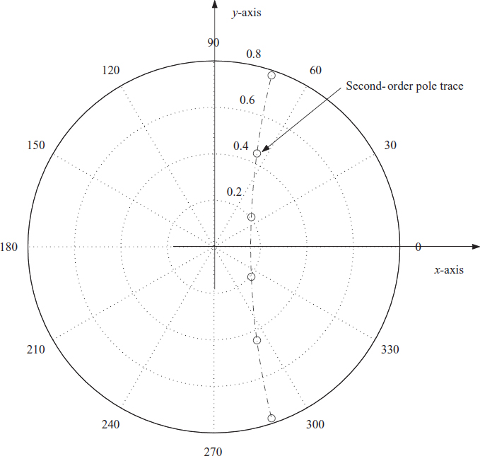
Figure 3.18 A Butterworth autoregressive filter

1. Cut-off frequency as 0.2 Hz;
2. Sixth-order filter giving a roll-off of 6 × 20 = 120 dB/decade
3. A permitted passband ripple of 0.4 dB

With these specifications, using the MATLAB package, we get the Chebyshev filter as

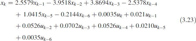
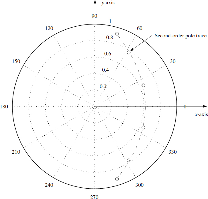
Figure 3.19 A Chebyshev autoregressive filter

A pole–zero plot of the same filter is shown in Figure 3.19. We can see that the desired filter is a cascade of second-order filters with poles following an equation x − 0.6168 = −0.4478y² and symmetric about the x-axis while three pairs of second-order zeros are positioned on the unit circle at 180⁰. It is very interesting to note that the poles are placed on a parabolic path with focal point towards the origin.

A filter with the same specifications except a flat passband characteristic is obtained using the Butterworth model, which results in

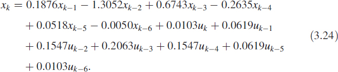
Unlike the pole–zero plot of the Chebyshev filter, we see that the focal point of the Butterworth filter plot is away from the origin. The pole trace follows the equation x − 0.1582 = 0.1651y², as shown in Figure 3.18. Once again, the zeros are positioned at 180° on the unit circle.

By now you have probably understood why we have focused on second-order filters. Almost all the filters can be realised by cascading second-order filters. For detailed design methods, consult a book on filter design.

3.8 Adaptive Filters

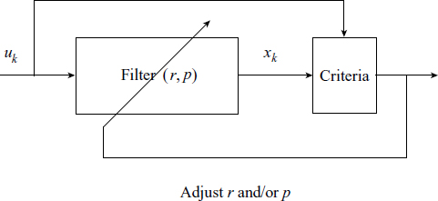
An Adaptive filter is a filter whose characteristics can be modified to achieve an objective by automatic adaptation or modification of the filter parameters. We illustrate this using a simple unity-gain BPF filter described in Section 3.4 via (3.17). We demonstrate this idea of adaptation by taking a specific criterion. In general, the criteria and the choice of feedback for adjusting parameters make an adaptive filter robust.

Figure 3.20 Adaptive filter

In this particular case, −2 ≤ p ≤ 2 since we have p = 2 cosθ. The parameter r is in (0,1). By choosing r = 1 the filter becomes marginally stable and this must be avoided.

3.8.1 Varying r

The effect of increasing the radial pole position r on the frequency response curve is that it becomes sharper and the amplitude increases. We also notice that as the value of r is reduced, the peak frequency changes. We show this by varying the value of r from 0.65 to 0.95. The value of p is kept constant at p = 1.5321 (θ = 40°). The plot is shown in Figure 3.21. The Peak frequency is related to the radial pole position r and the angular measure of the pole θ as

where θ_pk is peak angular frequency. Notice that when r → 1 we get θ_pk → θ.

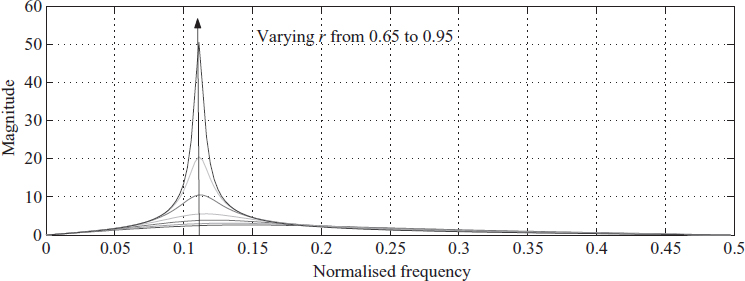
Figure 3.21 Filter response for varying values of r

3.8.2 Varying p

Another parameter which can be varied in the filter is p. So we increase the value of p while keeping r constant. From Figure 3.22 we find that the curve shifts towards the right as p increases. The value of p is varied from p = 1.6180 (θ = 36°) to p = −1.6180 (θ = 144°) keeping the value of r constant at 0.9. Thus we can conclude from the above curves that we can vary the filter characteristics by changing r or by changing p. But if we change the values of r continuously, then the value of r may exceed one. Under these conditions the system will become unstable, which is not desirable. To keep the system in a stable condition, we vary p. By varying θ we perform a non-linear variation. Hence we choose to vary the value of p = 2 cos θ. Thus frequency tracking can be done without changing the value of r and by varying p from −2 to 2 and fixing r at an optimum value.

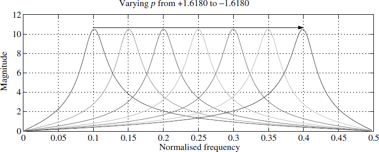
Figure 3.22 Filter response for varying values of p

3.8.3 Criteria

We have two parameters, r and p, in the filter. Suppose we need to adapt the filter so its output is maximum. This may sound vague but in a radio receiver we tune, or adjust, the frequency so the listening is best. We now know the sensitivity of the filter – how the parameter affects the characteristics of the filter and to what degree. We define a criteria function J(p), known as the objective function, as follows:

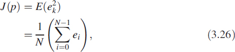
where e_k = x_k − u_k. Now we plot J(p) against parameter p (Figure 3.23). Notice that a minimum occurs at a single point. It is also essential that most of the time we must know the slope of this function given as S(p) = J(p).

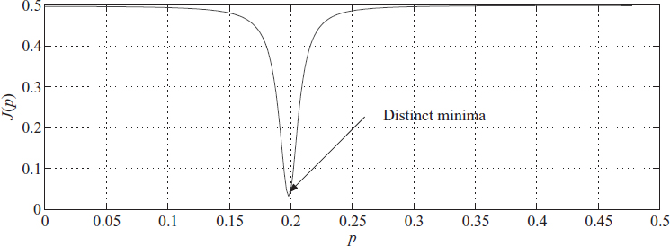
Figure 3.23 Criteria function J_(p)

This function is depicted in Figure 3.24. Perhaps you are wondering how these functions have been arrived at numerically. We describe this in greater detail in Chapter 6, where we give applications and some problems for research. In brief, the filter is excited by a pure sine wave and J(p) is computed using (3.26). Computing the slope of J(p) requires deeper understanding.

3.8.4 Adaptation

The most popular algorithm for adaptation is the steepest gradient method, also called the Newton–Raphson method. For incrementing the parameter p, we use the gradient J(p), defined as

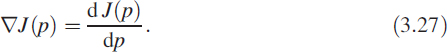
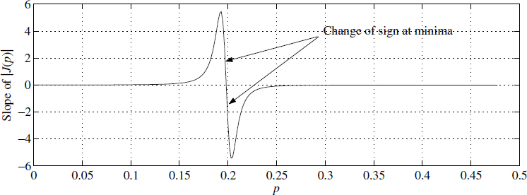
Figure 3.24 The slope of the criteria function is S(p) = ÑJ(p)

The parameter incrementing, adaptation or updating is performed as

Here μ is defined as the step size.

3.9 Demodulating via Adaptive Filters

Conventional coherent or non-coherent demodulation techniques for demodulation of binary frequency shift keyed (BFSK) signals do not perform well under low signal-to-noise ratio (SNR) conditions and knowledge of the frequencies poses a limitation. We analyse a demodulation technique in which a sampled version of a BFSK signal is passed through an adaptive digital notch filter. The filter estimates and tracks the instantaneous frequency of the incoming signal in the process of optimising an objective function; a smoothing of the estimated instantaneous frequencies followed by a hard decision gives the demodulated signal.

3.9.1 Demodulation Method

Consider a situation in which a BFSK signal, corrupted by zero-mean additive white noise, is sampled at the receiver. The sampled signal can be expressed as

where A is the amplitude (A > 0); γ_k is the additive noise, which is a zero-mean white random process with variance σ²; and f_k is the normalised instantaneous frequency (the actual instantaneous frequency divided by the sampling rate), given by

A typical FSK signal and its spectrum are given in Figure 3.25. As in the signal model (3.30), the SNR (in dB) is 10 log₁₀ (A²/2σ²). The signal is passed through an adaptive digital notch filter that consists of a digital bandpass filter (BPF) and a subtractor, along with a sensitivity function estimator and a parameter estimator. The sampled signal sequence {u_k} goes through a second-order BPF [6] whose output sequence {x_k} is governed by the second-order linear recurrence relation.

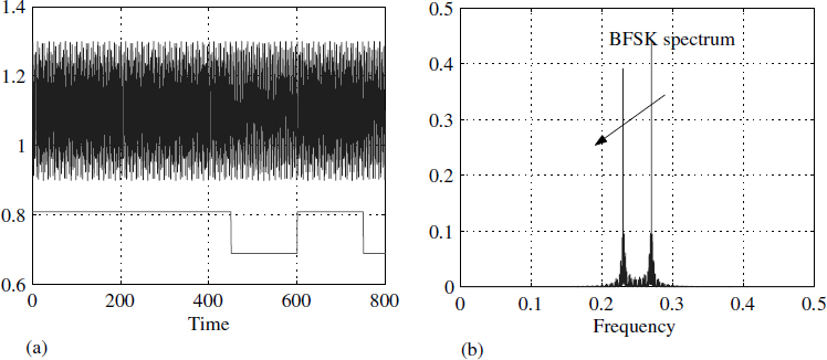
Figure 3.25 BFSK signal in the time domain and the frequency domain

where p = 2cosθ and θ is the normalised centre frequency of the BPF; r is the radial pole position. The subtractor subtracts the input u_k from the BPF output x_k to produce an error signal

The combination of the BPF and the subtractor with input sequence {u_k} and output sequence {e_k} is a notch filter. The parameter estimator estimates the parameter p for every k by trying to minimise the objective function

applying a gradient descent algorithm on p. Denoting the sensitivity function as

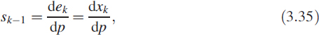
it can easily be shown that s_k satisfies the recurrence relation

In addition, if υ_k represents the mean of J_k(p), then υ_k can be computed recursively using an exponentially weighted fading function using the recurrence relation

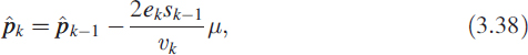
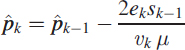
where λ, 0 < λ < 1, is the forgetting factor. Denoting as the estimate of p at time index k, we compute recursively as

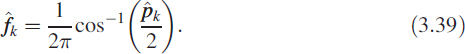
where μ is the step size. The instantaneous normalised frequency estimate is obtained from by the formula

The algorithm for obtaining the sequence {} of the estimates of the instantaneous normalised frequency from the sampled signal sequence {u_k} is as follows.

Choose parameters r, λ, μ and initial values x₀, x₋₁, u₀, u₋₁, s₀, s₋₁, s₋₂, υ₀, ₀ such that υ₀ > 0.

For k = 1,2, 3,…

1. 
2. 
3. 
4. 
5. 
6. 

By smoothing the sequence {} and then performing a hard decision on the smoothed sequence, we obtain the demodulated signal. We have chosen to pass the signal {} through a hard limiter to reduce the computational burden, which is a requirement in real-time embedded system software development.

3.9.2 Step Size μ

In all the methods the choice of μ plays an important role. Various authors [5] have adopted different techniques for the choice of μ. From the value of s_k we can obtain the incremental value of p. A sign change in the slope of a function indicates that a minimum or maximum occurs in between these points. Hence to find the minimum for the function given by (3.34), we need to find the sign change in the slope of J_k(p) ≅ E{e_ks_k}. Let us define a variable α_k such that

which may take the value −1 or +1 depending on J_k(p). We change the step size μ to half its original value if we see any change in α_k. In other words, if

it implies that a sign change has occurred and the value of μ changes as

otherwise

By changing the value of μ for a change in α_k, the value of p converges to the precise value in fewer iterations.

3.9.3 Performance

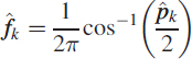
A signal with additive noise such that the SNR of the signal is 10 dB is implemented for different normalised frequencies of the incoming signal from 0.1 to 0.4 at SNR = 10 dB. A few values are shown in Table 3.1. It shows the performance of the algorithm expressed as the nominal mean and its deviation from the true value as an error. The algorithm is now used to demodulate an FSK by tracking the mark and space frequencies. An implementation for an FSK signal with SNR = 10 dB is shown in Figure (3.26).

Table 3.1 Performance of the algorithm

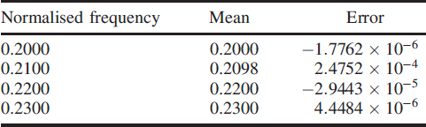
Figure 3.26 Demodulated BFSK signal p

3.10 Phase Shift via Adaptive Filter

In the application of detection, array processing and direction finding, we need to take the given narrowband signal (here we have chosen a sinusoidal wave) and shift it by a given value. The following example generates a π/2 phase shift by adjusting the coefficient of the first-order all-pass filter. Consider the given signal u_k as

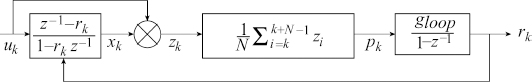
Figure 3.27 Adaptive phase shifting

u_k = cos(2πfk + ϕ) where f is the normalised frequency and ϕ is an arbitrary phase value. Figure 3.27 depicts the macro view of the filter.

The above filter is implemented for N = 40, g_loop = 0.01 and 1/f = 77 with ϕ = π/20 and an initial value of r_k = 0.2. Figure 3.28 shows the phase shift.

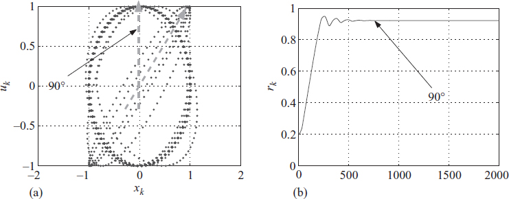
Figure 3.28 Phase shifting by an adaptive filter

3.11 Inverse Problems

Inverse problems are classified under parameter estimation. Originally the playground of statisticians, people from many disciplines have now entered this field. It is best used for many applications in DSP.

In general, it is a complex problem to find the difference equation or the digital filter that yields the given output for a given input, and a solution cannot be assured. Often a unique solution is impossible. Each problem must be treated individually. However, we will describe a generic method and enumerate the shortcomings. This is a fairly big area, so it is not possible to do more than give a few relevent pointers. Chapter 6 gives some applications using this idea.

There are two problems in this area: non-availability of knowledge of the filter order, and the presence of noise in measurements. These make the solution difficult.

3.11.1 Model Order Problem

Let us consider two digital filters:

Look at Figure 3.29(a) and (b). They represent the frequency responses of the digital filters in (3.49) and (3.50). We have superimposed the two responses in Figure 3.29(b). Notice that there is a good match in an engineering sense.

Multiple solutions make life more complicated in inverse problems. The reason for this is that both filters have different phase responses or could have a pole-zero cancellation. One of the best criteria for fixing the model order is by Akaike, known as the Akaike information criterion (AIC). Given an input sequence {u_k} and output sequence {y_k}, using AIC and human judgement, by looking at the spectrum of {y_k}, we can arrive at a fairly accurate estimate for p and q in (2.15), where p is the order of the numerator polynomial and q is the order of the denominator polynomial.

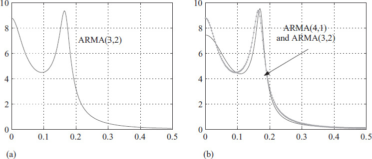
Figure 3.29 Two different filters give the same frequency response

3.11.2 Estimating Filter Coefficients

Refer to (1.24) to (1.26) for the definition of the vector p = [a₁,a₂,…,a_p,b₁,…,b_q]which defines the digital filter. We also have another vector . Then we construct an equation representing the given data as . This is exactly the same as the set of overdetermined simultaneous equations given in Chapter 2 and the solution has the form of (2.35). Using (2.36) and (2.33), we arrive at the solution for p as

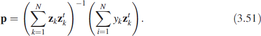
There are many methods centred around this solution and they are shown in Figure 3.29A.

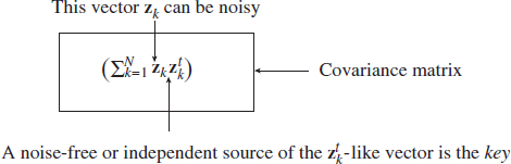
Figure 3.29A There are many methods centred around solution (3.51)

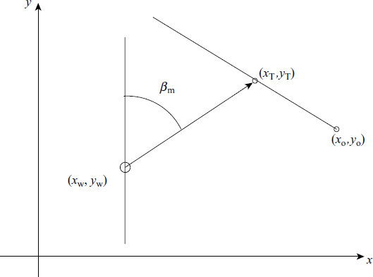
Figure 3.30 Tracking a moving object

3.11.3 Target Tracking as an Inverse Problem

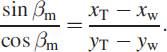
In real life, formulation of a problem constitutes 50% of the solution. Let us consider an object moving with a uniform speed in a straight line (Figure 3.30). At t = 0, or in the discrete-time domain at k = 0, we assume it has a value of (x₀,y₀). We observe the target coordinates (x_T, y_T) from a movable watching place at (x_w, y_w). The angle with respect to the true north is β_m = tan⁻¹[(x_T − x_w)/(y_T − y_w)].

3.11.3.1 Problem Formulation

We can recast the problem as

We rewrite the equation as

Under the assumption that the target is travelling at uniform speed in a constant direction, we get x_t = x_o + k δt υ_x and y_T = y_o + k δt υ_y, which leads to

To bring this into standard form, we put

and b^t = [x_o y_o ν_x ν_y]. Representing the output as a scalar y_k = x_w cos β_m − y_w sin β_m, we get

3.11.3.2 Pseudolinear Solution

The above formulation is a pseudo MA filter. This is an inverse problem of finding b given y_k and u. The solution can be of block type or recursive type. For simplicity we show a block solution which is given as ; it is depicted in Figure 3.31(a). It shows the motion of the watcher or observer, the motion of the target and the estimated motion of the target. Figure 3.31(b) shows the angle (β_m) measurements.

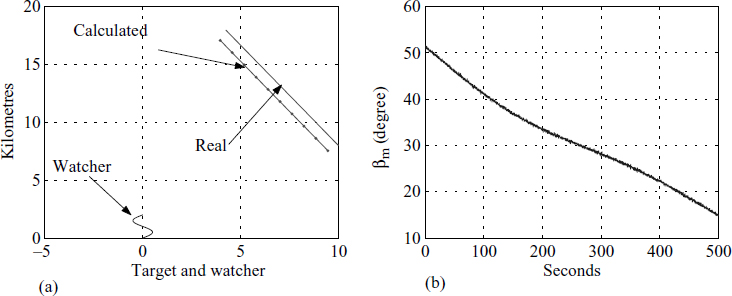
Figure 3.31 Watcher and target in (3.54)

A careful look at Figure 3.31(a) reveals that the estimate is biased, even though the direction is correct. This is because we have introduced a small amount of noise in the measured angle β_m. In fact, it is a very small bias but still significant. A considerable amount of published work is available in the area known as target motion analysis (TMA). There are many methods to remove this bias, such as instrumental variable (IV) methods, maximum likelihood (ML) methods and IV approximate ML (IVAML) estimators. There are many associated problems still to be researched.

3.12 Kalman Filter

The output of a filter is completely characterised by its coefficients and the initial conditions (Figure 3.31A).

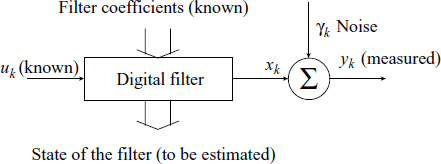
Figure 3.31A Kalman filter: the output is completely characterised by the filter coefficients and the initial conditions

For a simple explantion, consider (3.16), where the infinite sequence is generated by a 3-tuple {1.8,1,0} in which there are two components: coefficients, known as parameters; and the other values at various places inside the filter before the delay elements, known as the state of the filter.

The output is generally a linear combination of these states. The aim of the Kalman filter is to accurately estimate these states by measuring the noisy output. The following examples illustrate the approach and its application.

3.12.1 Estimating the Rate

Estimating the rate occurs in radar, tracking and control. Let us consider a sequence of angular measurements {θ₁, θ₂,…, θ_N} over a relatively small window.

It is required to find the slope or the rate. The problem looks simple, but using conventional Newton forward or backward differences produces noisy rates. Consider the simple plot of θ_k in Figure 3.32.

Now we place the x and y axes at the desired point, as shown in Figure 3.32. Note that we have moved only the y-axis to the desired place. Then we have θ = mk δt + c. Here we need to estimate the value of m. This choice of coordinate frame ensures that k = 0 at all times. We can write

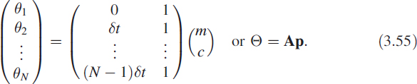
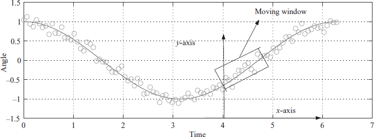
Figure 3.32 Linear regression over a rectangular moving window

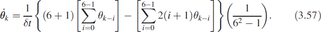
Now the solution for such overdetermined equations in a least-squares sense is p = (A^tA)⁻¹ A^tΘ, where our interest is p(1) = m. We can derive a closed-form solution as

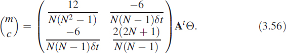
Even though (3.56) looks very complicated, it is only a pair of FIR filters with their impulse responses given as = {2,4,6, 8,…} and = {1,1,1,1,…}. For a six-point moving linear regressor, the rate is given as

This is shown in Figure 3.33, which is a SIMULINK block diagram. In fact, this is a Kalman filter or a state estimator.

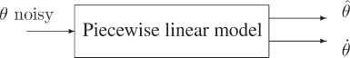
3.12.2 Fitting a Sine Curve

There are many situations where you know the frequency, but unfortunately, by the time you get the signal, it is corrupted and of the form y_k = sin(2πfk) + n_k, where n_k is a zero-mean uncorrelated noise. The problem is to get back the original signal. Immediately what strikes our mind is a high-Q filter. Unfortunately, stability is an issue for these filters. In situations of this type, we use model-based filtering. Consider an AR process representing an oscillator (poles on the unit circle):

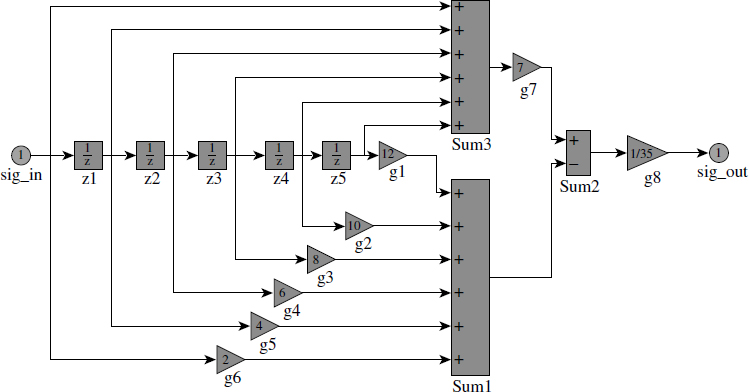
Figure 3.33 Moving linear regression

The parameter p has a direct relationship with the frequency. We can see that the initial conditions of this difference equation uniquely determine the amplitude and phase of the desired noise-free sine wave. Now we aim at finding out the initial conditions of this difference equation that generate the best-fit sine wave matching the noisy generated sine wave (Figure 3.34). To formulate this problem, we choose to write it as

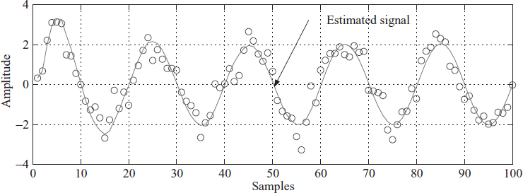
Figure 3.34 Fitting a sine curve to a noisy signal

We also define a vector c^t = (1 0). Then the noisy measured signal will be y_k = c^tΘx_k−1 + n_k. Now let the unknown initial condition vector be x₀. Then we have

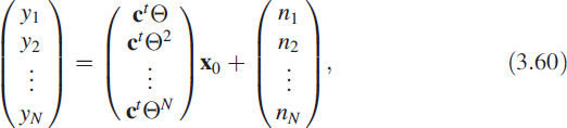
which is of the form y = Ax₀ + n. Now we know that the least-squares solution for the initial conditions of the oscillator is x₀ = (A^tA)⁻¹A^ty.

We do not need to do these computational gyrations. Fortunately, we can use a fine numerically efficient recursive method known as a Kalman filter. The following set of equations provide a recursive solution and update the desired estimate of the signal ŷ_k on receipt of new data:

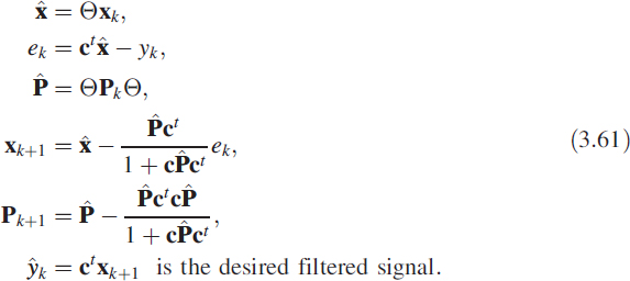
We recommend you to look at the above as a numerical method for implementing

The choice of P₀ = 10⁻³I is good and we can start with any arbitrary value of x_k. Programs given in the appendix will throw more light on this.

3.12.3 Sampling in Space

Consider an antenna consisting of the uniform linear array (ULA) shown in Figure 3.35. We assume a radiating narrowband source transmitting in all directions. The signal as seen by the ULA at a given instant of time is a sine wave or part of it, depending on the interelement spacing. For this reason it is called sampling in space. The set of signals measured by the ULA is noisy and given as y_n = x_n + γ_n, where γ_n is a zero-mean uncorrelated random sequence.

This example aims at obtaining a set of coefficients for a pair of FIR filters which satisfy the property that the output of the filter pair acts as a state estimate for a sinusoidal oscillator. These coefficients are then modified and applied to a direction finding (DF) system using a ULA.

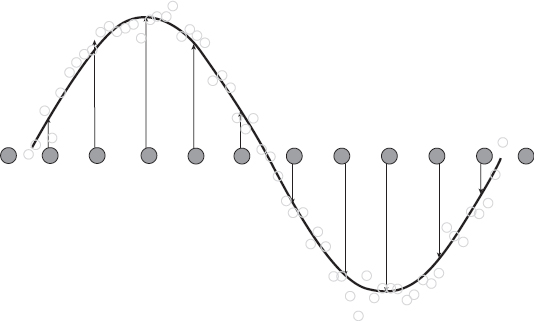
Figure 3.35 Spatial wave on a ULA of L measurements y_1,n, K, y_L,n

3.12.3.1 Angular Frequency Estimation

Consider an AR process given by

representing an oscillator with normalised angular frequency . By defining

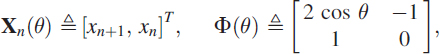
this can be rewritten as X_n(θ) = Φ(θ)X_n−1(θ) where X_n(θ) is the state vector and (θ) is the state transition matrix. For the nth snapshot (n = 1,…, N) let L measurements y_1,n,…, y_L,n of x_n,…, x_n+L−1 be written as

where [0, 1]^T, and γ_k,n is additive noise. An L × 1 measurement vector

can be expressed using (3.63) as

where Γ_n is the additive noise vector, and

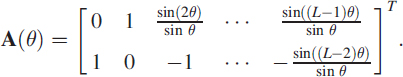
The least squares estimate (LSE) of X_n(θ) in (3.64) is

Each row of the weighting matrix [A^T(θ)A(θ)]⁻¹A^T(θ) represents an FIR filter of L coefficients.

Consider a measurement vector Y_n(ω) for an oscillation at ω. If X_n(ω) is computed using Φ(θ), then its LSE is given by A^T (θ)Y_n(ω). The estimate of Y_n(ω) is then

3.13 Summary

This chapter described ways to specify a given filter. We presented a variety of popular filters and their characteristics. We looked at IIR filters with real coefficients and truncated IIR filters for use in FIR designs. We also described a bank of filters with complex coefficients pointing to discrete Fourier transforms. We gave a simple presentation of adaptive filters and inverse problems having practical significance. We demonstrated an application of BFSK demodulation and adaptive phase shifting. And we looked at a practical inverse problem from target tracking. We added an important dimension by giving Kalman filter applications. Then we concluded this big topic with an application from array processing.

References

1. R. W. Hamming, Digital Filters, pp. 4–5. Englewood Cliffs, NJ: Prentice Hall, 1980.

2. R. D. Strum and D. E. Kirk, First Principles of Discrete Systems and Digital Signal Processing. Reading MA: Addison-Wesley, 1989.

3. K. V. Rangarao, Adaptive digital notch filtering. Master's thesis, Naval Postgraduate School, Monterey CA, September 1991.

4. G. C. Goodwin and K. S. Sun, Adaptive Filtering, Prediction and Control. Englewood Cliffs NJ: Prentice Hall, 1984.

5. D. M. Himmelblau Applied Non-linear Programming. New York: McGraw-Hill, 1972.

6. K. Kadambari, K. V. Rangarao and R. K. Mallik, Demodulation of BFSK signals by adaptive digital notch filtering. In proceedings of the IEEE International Conference on Personal Wireless Communications, Hyderabad, India, December 2000, pp. 217–19.