1

Processing of Signals

Any sequence or set of numbers, either continuous or discrete, defines a signal in the broad sense. Signals originate from various sources. They occur in data processing or share markets, human heartbeats or telemetry signals, a space shuttle or the golden voice of the Indian playback singer Lata Mangeshkar, the noise of a turbine blade or submarine, a ship or instrumented signal inside a missile.

Processing of signals, whether analogue or digital, is a prerequisite to understanding and analysing them. Conventionally, any signal is associated with time. Typically, a one-dimensional signal has the form x(t) and a two-dimensional signal has the form f (x, y, t). Understanding the origin of signals or their source is of paramount importance. In strict mathematical form, a signal is a mapping function from the real line to the real line, or in the case of discrete signals, it is a mapping from the integer line to the real line;¹ and finally it is a mapping from the integer line to the integer line.

Typically the measured signal ŷ(t) is different from the emanated signal y(t). This is due to corruption and can be represented as follows:

where γ is the unwanted signal, commonly referred to as noise and most of the time statistical in nature. This is one of the reasons why processing is performed to obtain ŷ_k from y_k.

1.1 Organisation of the Book

Chapter 1 describes how analogue signals are converted into numbers and the associated problems. It gives essential principles of converting the analogue signal to digital form, independent of technology. Also described are the various domains in which the signals are classified and the associated mathematical transformations. Chapter 2 looks at the basic ideas behind the concepts and provides the necessary background to understand them. Chapter 2 will give confidence to the reader to understand the principles of digital filters. Chapter 3 describes commonly used filters along with practical examples. Chapter 4 focuses on Fourier transform techniques plus computational complexities and variants. It also describes frequency domain least squares in the spectral domain. Chapter 5 looks at methodologies of implementing the filters, various types of converters, limitations of fixed points and the need for pipelining. We conclude by comparing the commercially available processors and by looking at implementations for two practical problems: a DSP processor and a hardware implementation using an FPGA.² Chapter 6 describes a system-level application in two domains. The MATLAB programs in the appendices may be modified to suit readers' requirements.

1.2 Classification of Signals

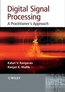
Signals can be studied using spectral characteristics and temporal characteristics. Figure 1.1 shows the same signal as a function of time (temporal) or as a function of frequency (spectral). It is very important to understand the signals before we process them. For example, the sampling for a narrowband signal will probably be different than the sampling for a broadband signal. There are many ways to classify signals.

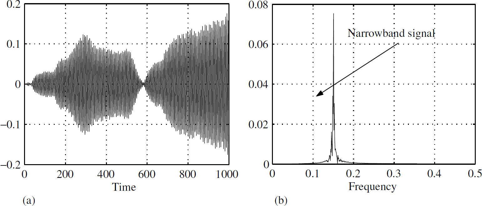
Figure 1.1 Narrowband signal x(t)

1.2.1 Spectral Domain

Signals are generated as a function of time (temporal domain) but it is often convenient to analyse them as a function of frequency (spectral domain). Figure 1.1 shows a narrowband signal in the temporal domain and the spectral domain. Figure 1.2 does the same for a broadband signal. For historical reasons, signals which are classified by their spectral characteristics are more popular. Here are some examples:

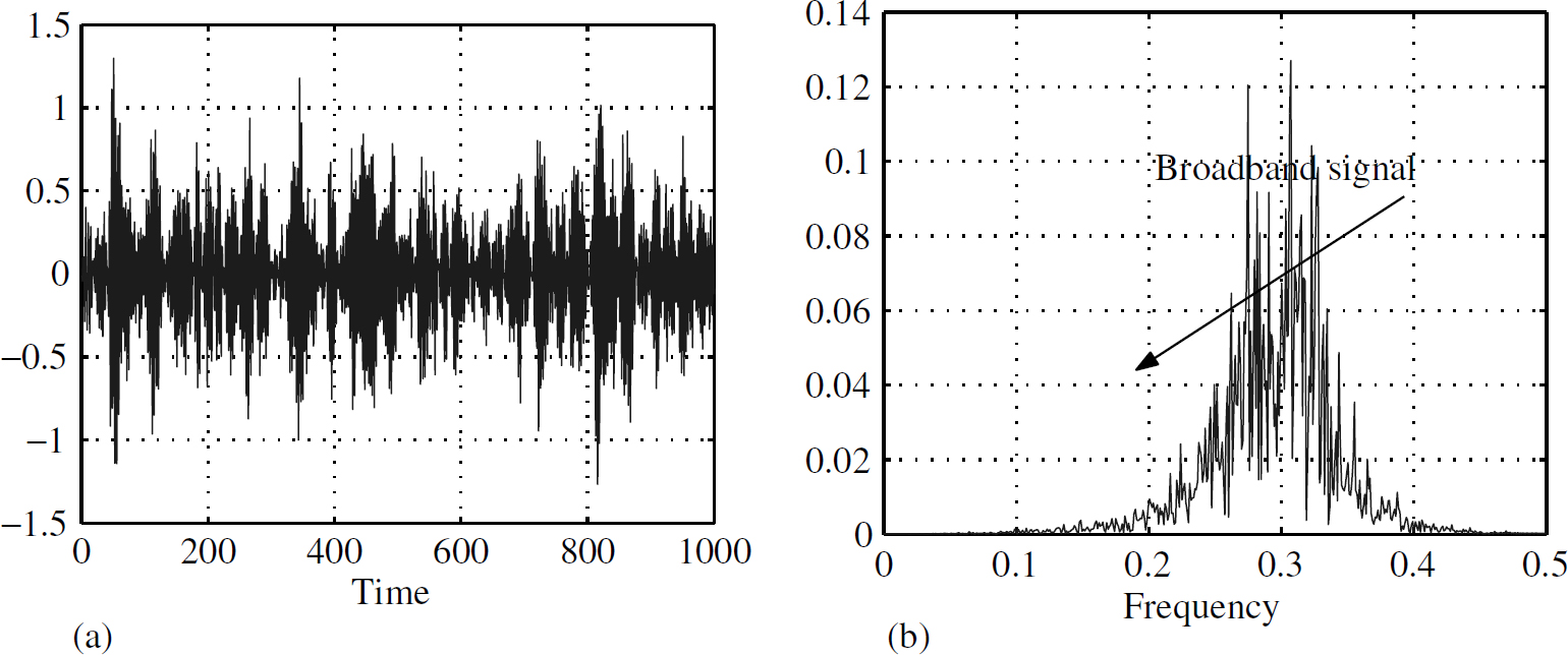
Figure 1.2 Broadband signal x(t)

1. Band-limited signals

   (a) Narrowband signals

   (b) Wideband signals

2. Additive band-limited signals

1.2.1.1 Band-Limited Signals

Band-limited signals, narrow or wide, are the most commonly encountered signals in real life. They could be a signal from an RF transmitter, the noise of an engine, etc. The signals in Figures 1.1 and 1.2 are essentially the same except that their bandwidths are different and cannot be perceived in the time domain. Only by obtaining the spectral characteristics using the Fourier transform we can distinguish one from the other.

1.2.1.2 Additive Band-Limited Signals

A group of additive band-limited signals are conventionally known as composite signals with a wide range of frequencies. Typically, a signal emitted from a radar [1] and its reflection from the target have a carrier frequency of a few gigahertz and a pulse repetition frequency (PRF) measured in kilohertz. The rotation frequency of the radar is a few hertz and the target spatial contour which gets convolved with this signal is measured in fractions of hertz.

Composite signals are very difficult to process, and demand multi-rate signal processing techniques. A typical composite signal in the time domain is depicted in Figure 1.3(a), which may not give total comprehension. Looking at the spectrum of the same signal in Figure 1.3(b) provides a better understanding. These graphs are merely representative; in reality it is very difficult to sample composite signals due to the wide range of frequencies present at logarithmic distances.

Figure 1.3 Composite signal x(t)

1.2.2 Random Signals

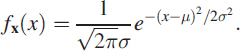
Only some signals can be characterised in a deterministic way through their spectral properties. There are some signals which need a probabilistic approach. Random signals such as shown in Figure 1.4(a) can only be characterised by their probability density function (pdf). For the same signal we have estimated the pdf by a simple histogram (Figure 1.4(b)). For this signal we have actually generated the pdf from the given time series using a numerical technique; notice how closely it matches with the theoretical bell-shaped curve representing a normal distribution.

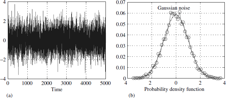
Figure 1.4 Random signal x(t) with pdf

Statistical or random signals can also be characterised only by their moments, such as first moment (mean μ), second moment (variance σ²) and higher-order moments [8]. In general, a statistical signal is completely defined by its pdf and in turn this pdf is uniquely related to the moments. In some cases the entire pdf can be generated using only μ and σ², as in the case of a Gaussian distribution, where the pdf of a Gaussian random variable x is given by

The pdf does not have to be static; it could vary with time, making the signal non-stationary.

1.2.3 Periodic Signals

A signal x(t) is said to be periodic if

The periodicity of x(t) is min(nT), which is T. If we rewrite this using the notation t = k δt, where k is an integer and δt is a real number,³ then

We write the quantity T/δt = + ∈, where ∈ is a real number⁴ less than 1 and is an integer. The practising engineer's periodicity in a loose sense is ; in a strict mathematical sense the periodicity min [n( + ∈ )] = N must be an integer. N could be very different from or may not exist. This illustrates that periodicity is not preserved while moving from the continuous domain to the discrete domain in all cases in a strict sense.

1.3 Transformations

The sole aim of this section is to introduce two common signal transformations. A detailed discussion is available in later chapters of this book. Signals are manipulated by performing various mathematical operations for better understanding, presentation and visibility of the signal.

1.3.1 Laplace and Fourier Transforms

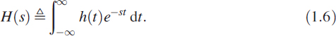
One such transformation is the Laplace transform (LT). If h(t) is a time-varying signal, which is a function of time t, then the Laplace transform⁵ of h(t) is denoted as H(s), where s is a complex variable, and is defined as

The complex variable s is often denoted as σ + jω, where . σ is the real part of s and represents the rate of decay or rise of the signal. ω is the imaginary part of s and represents the periodic variation or frequency of the signal. The variable s is also sometimes called the complex frequency.

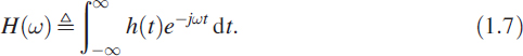
When we are interested only in the frequency content of the signal h(t), we use the Fourier transform, which is denoted⁶ H(ω) and given by

In fact, combining the above equation with the Euler equation,⁷ we can derive the Fourier series, which is a fundamental transformation for periodic functions.

These transformations are linear in nature, in the sense that the Laplace or Fourier transform of the sum of two signals is the sum of their transforms, and the Laplace or Fourier transform of a scaled version of a signal by some time-independent scale factor is the scaled version of its transform by the same scale factor.

1.3.2 The z-Transform and the Discrete Fourier Transform

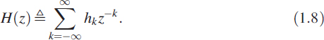
When we move from the continuous-time domain to the discrete-time domain, integrands get mapped to summations. Replacing e^s with z and h(t) with h_k in (1.6), we get a new transform in the discrete-time domain known as the z-transform, one of the powerful tools representing discrete-time systems. The z-transform of a discrete-time signal h_k is denoted as H(z) and is given by

As a simple illustration, consider a sequence of numbers

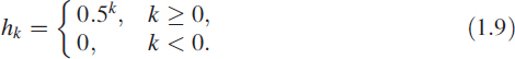
Using (1.8) for the sequence h_k we get

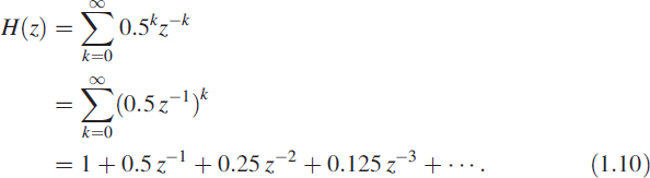
Using the simple geometric progression relation

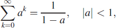
we get

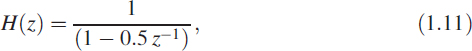
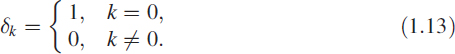
under the condition |0.5z⁻¹| < 1, that is, |z| > 0.5. Note that this condition represents the region of the complex z-plane in which the series (1.10) converges and (1.11) holds, and is called the region of convergence (ROC). We can also write h_k in the form

where δ_k is the Kronecker delta function, given by

If, instead of the variable z, we use the variable e^jΩ, where Ω is the frequency, then we get the discrete fourier transform (DFT), which is defined as

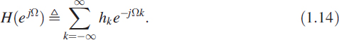
The z-transform is thus a discrete-time version of the Laplace transform and the DFT is a discrete-time version of the Fourier transform.

1.3.3 An Interesting Note

We have started with an infinite sequence h_k (1.9) which is also represented in the form H(z), known as the transfer function (TF), in (1.11) and in a recursive way in (1.12). Thus we have multiple representations of the same signal. These representations are of prime importance and constitute the heart of learning DSP; greater details are provided in later chapters.

1.4 Signal Characterisation

The signal y_k of (1.2) could be any of the signals in Figures 1.1, 1.2 or 1.3 and it could be characterised in the frequency domain by the non-parametric spectrum. This spectrum is popularly known as the Fourier spectrum and is well understood by everyone. The same signal can also be represented by its parametric spectrum, computed from the parameters of the system where the signal originates.

Signals per se do not originate on their own; generally a signal is the output of a process defined by its dynamics, which could be linear, non-linear, logical or a combination. Most of the time, due to our limitations in handling the information, we assume a signal to be the output of a linear system, either represented in the continuous-time domain or the discrete-time domain. In this book, we always refer to discrete-time systems. In computing the parametric spectrum, we aim to find the system which has an output of a given signal, say y_k. This constitutes a separate subject known as parameter estimation or system identification.

1.4.1 Non-parametric Spectrum or Fourier Spectrum

If the signal y_k of (1.2) is known for k = 1, 2, …, N, it can also be represented as a vector

where (·)^T denotes transpose, which can be transformed into the frequency domain by the DFT relation

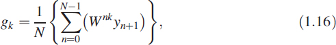
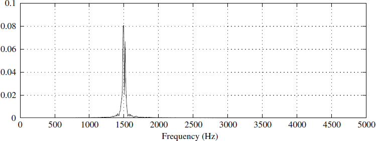
Figure 1.5 Fourier power spectrum s(k)(1.17)

where W = e^−j2π/N. In general g_k is a complex quantity. However, we restrict our interest to the power spectrum of the signal y_k, a real non-negative quantity given by

where (·)* represents the complex conjugate and | · | represents the absolute value (Figure 1.5). The series S_N, given by

is another way of representing the signal. Even though the signal in the power spectral domain is very convenient to handle, other considerations such as resolution, limit its use for online application. Also, in this representation, the phase information of the signal is lost.

To preserve the total information, the complex quantity g_k is represented as an ordered pair of time series, one representing the in-phase component and the other representing the quadrature component:

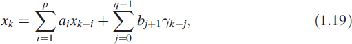
1.4.2 Parametric Representation

In a parametric representation the signal y_k is modelled as the output of a linear system which may be an all-pole or a pole-zero system [2]. The input is assumed to be white noise, but this input to the system is not accessible and is only conceptual in nature. Let the system under consideration be

where γ_k is white noise and y_k is the output of the system. Equation (1.19) can also be represented as a transfer function (TF) [3, 4]:

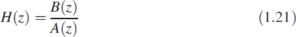
or

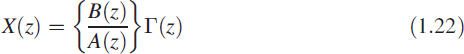
or in the delay operator notation⁸

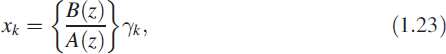
where X(z) and Γ(z) are the z-transforms of x_k and γ_k, respectively, and

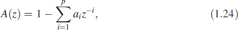
are the z-transforms of {1, −a₁, −a₂, …, −a_p} and {b₁, b₂,…, b_q}, respectively. We define the parameter vector as

The parameter vector p completely characterises the signal x_k. The system defined by (1.19) is also known as an autoregressive moving average (ARMA) model [1, 6]. Note that the TF H(z) of this model is a rational function of z⁻¹, with p poles and q zeros in terms of z⁻¹. An ARMA model or system with p poles and q zeros is conventionally written ARMA (p, q).

1.4.2.1 Parametric Spectrum

Given the parameter vector p (1.26) we obtain the parametric spectrum |H(e^jω)| as

Using the given value of p, we obtain the parametric spectrum via (1.28). The function |H(e^jω)| is periodic (with period 2π) in ω.

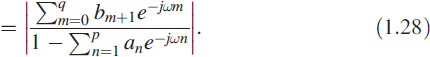
When the parameter vector p is real-valued, |H(e^jω)| is also symmetric in ω, and we need to evaluate (1.28) only for 0 < ω < π. Figure 1.6 is the parametric spectrum of the narrowband signal. We have obtained this spectrum by first obtaining the parameter vector p (1.26) of the given time series and substituting this value in (1.28).

Figure 1.6 Parametric spectrum ||H(e^jw)|| using (1.28)

1.5 Converting Analogue Signals to Digital

An analogue signal y(t) is in reality a mapping function from the real line, to the real line, defined as → , where denotes the set of real numbers. When converted to a digital signal, this function goes through transformations and becomes modified into another signal which mostly preserves the information, depending on how the conversion is done. The process of modification or morphing has three distinct stages:

• Windowing
• Digitisation: sampling
• Digitisation: quantisatioin

1.5.1 Windowing

The original signal could be very long and non-periodic, but due to physical limitations we observe the signal only for a finite duration. This results in multiplication of the signal by a rectangular window function R(t), giving an observed signal

where

T_w is the observation time interval. In general, R(t) can take many forms and these functions are known as windowing functions [5].

1.5.2 Sampling

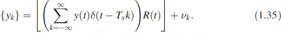
In reality, a band-limited analogue signal y(t) needs to be sampled, resulting in a discrete-time signal {y_k}, converting the function as a mapping from the integer line to the real line → , where denotes the set of integers. We express {y_k} as

where δ(t) is the unit impulse (Dirac delta function)

T_s is the sampling time. The sampling process is defined via (1.31) and is shown in Figure 1.7(a). This process generates a sampled or discrete signal. The Fourier transform of the sampled signal y_k (Figure 1.7(b)) is computed and shown in Figure 1.8.

The striking feature in Figure 1.8 is the periodic replication of the narrowband spectrum. Revisiting Fourier series will help us to understand the effect of sampling. The Fourier series is indeed a discrete spectrum or a line spectrum, and results from the periodic nature of a signal in the time domain. Any transformation from the time domain to the frequency domain maps periodicity into sampling, and vice versa. What it means is that sampling in the time domain brings periodicity in the frequency domain, and vice versa, as follows.

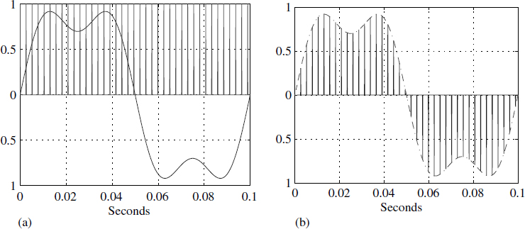
Figure 1.7 Discrete signal generation via (1.31)

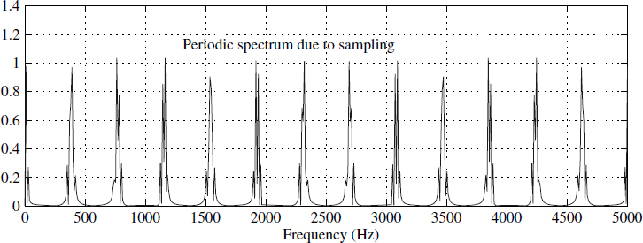
Figure 1.8 Spectrum of sampled signal y_k

Time domain	Frequency domain
Sampling Periodicity	Periodicity Sampling

In fact, the Poisson equation depicts this as

where S_y(·) is the Fourier spectrum of the signal y(t), which is periodic in f with period , shown in Figure 1.8.

1.5.2.1 Aliasing Error

A careful inspection of (Equation 1.33 and Figure 1.8) shows there is no real loss of information except for the periodicity in the frequency domain. Hence the original signal can be reconstructed by passing it through an appropriate lowpass filter. However, there is a condition in which information loss occurs, which is 1/T_s ≥ 2f_c, where f_c is the cut-off frequency of the band-limited signal. If this condition is not satisfied, a wraparound occurs and frequencies are not preserved. But this aliasing is put to best use for downconverting the signals without using any additional hardware, like mixers in digital receivers, where the signals are bandpass in nature.

1.5.3 Quantiaation

In addition, the signal gets quantised due to finite precision analogue-to-digital converters. The signal can be modelled as

where is a finite quantised number and ν_k is a uniformly distributed (UD) random number of LSB. Sampled signal y_k and are depicted in Figure 1.9(a) and the quantisation error is shown in Figure 1.9(b). In this numerical example we have used 10 (±5) levels of quantisation, giving an error (γ_k) between , which can be seen in Figure 1.9(b). The process of moving⁹ signal from one domain to the other domain is as follows:

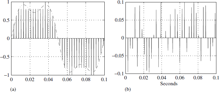
Figure 1.9 Quantised discrete signal |y_k|

In reality we get only windowed, discrete and quantised signal at the processor. Figure 1.10 depicts a 4-bit quantised, discrete and rectangular windowed signal.

Figure 1.10 Windowed discrete quantised signal

1.5.4 Noise Power

The sample signal y_k on passing through a quantiser such as an analogue-to-digital (A/D) converter results in a signal , and this is shown in Figure 1.9 along with the quantisation noise. The quantisation noise is a random variable (rv) with uniform distribution. The variance σ² is given as (1/12)(2⁻ⁿ)², where n is the length of the quantiser in bits. The noise power in decibels (dB) is given as 10 log σ² = −10 log(12) − [20 log(2)]n. If we assume that the signal y_k is equi-probable along the range of the quantiser, it becomes a uniformly distributed signal. We can assume without any loss of generality the range as 0 to 1. Then the signal power is 10 log(12). The signal-to-noise ratio (SNR) is 20n log(2) dB or 6 dB per bit.

Mathematically, the given original signal got corrupted due to the process of sampling and converting into physical world, real numbers. These are the theoretical modifications alone.

1.6 Signal Seen by the Computing Engine

With so much compulsive morphing, the final digitised signal¹⁰ takes the form

. modelling of Discrete Signal

In (1.35) we have not included any noise that gets added due to the channel through which the signal is transmitted. Besides that, in reality the impulse function δ(t) is approximated by a narrow rectangular pulse of finite duration.

1.6.1 Mitigating the Problems

Quantisation noise is purely controlled by the number of bits of the converter. The windowing effect is minimised by the right choice of window functions or choosing data of sufficient duration. There are scores of window functions [5] to suit different applications.

1.6.1.1 Anti-Aliasing Filter

It is necessary to have a band-limited signal before converting the signal to discrete form, and invariably an analogue lowpass filter precedes an A/D converter, making the signal band-limited. The choice of the filter depends on the upper bound of the sampling frequency and on the nature of the signal.

1.6.2 Anatomy of a Converter

There are three distinct parts to an A/D converter, as shown in Figure 1.11:

• Switch
• Analogue memory
• Conversion unit

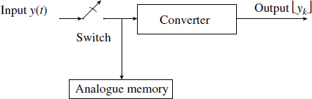
Figure 1.11 Model of an A/D converter

The switch is controlled by an extremely accurate timing device. When it is switched on it facilitates the transfer of the input signal y(t) at that instant to an analogue memory; after transfer, it is switched off, holding the value, and conversion is initiated. In specifying an A/D device there are four important timings: on time t_on of the switch is a non-zero quantity, because any switch takes a finite time to close; hold time t_hold is the period when the signal voltage is transferred to analogue memory; off time t_off is also non-zero, because a switch takes a finite time to open; finally, there is the conversion time t_c.

The sampling time T_s is the sum of all these times, thus T_s = t_on + t_hold + t_off + t_c. As technology is progressing, the timings are shrinking, and with good hardware architecture, sampling speeds are approaching 10 gigasamples per second with excellent resolution (24-bit). Way back in 1977 all these units were available as independent hardware blocks. Nowadays, manufacturers are also including anti-aliasing filters in A/D converters, apart from providing as a single chip.

There are many conversion methods. The most popular ones are the successive approximation method and a flash conversion method based on parallel conversion, using high slew rate operational amplifiers. A wide range of these devices are available in the commercial market.

1.6.3 The Need for Normalised Frequency

We enter the discrete domain once we pass through an A/D converter. We have only numbers and nothing but numbers. In the discrete-time domain, only the normalised frequency is used. This is because, once sampling is performed and the signal is converted into numbers, the real frequencies are no longer of any importance. If f_actual is the actual frequency, f_n is the normalised frequency, and f_s is the sampling frequency, then they are related by

Due to the periodic and symmetric [2] nature of the spectrum, we need to consider f_n only in the range 0 < f_n < 0.5. This essentially follows from the Nyquist theorem, where the minimum sampling rate is twice the maximum frequency content in the signal.

1.6.4 Care before Sampling

Once the conversion is over, damage is either done or not done; there are no halfway houses. Information is preserved or not preserved. All the care must be taken before conversion.

1.7 It Is Only Numbers

Once the signal is converted into a set of finite accurate numbers that can be represented in a finite-state machine, it is only a matter of playing with numbers. There are well-defined, logical, mathematical or heuristic rules to play with them. To demonstrate this concept of playing (Figure 1.12), we shall conclude this chapter with a simple example of playing with numbers.

Figure 1.12 It is playing with numbers

Let {y_k} = {y₁, y₂,…} be a sequence of numbers so acquired. Its mean at discrete time k is defined as

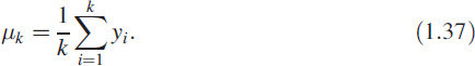
The above way of computing the mean is known as a moving-average process. We recast the (1.37) as and for k + 1 we write it as

We can rewrite (1.39) as

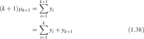
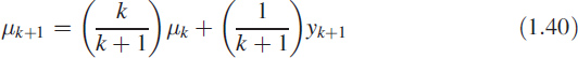
It can easily be seen that (1.41) is a recursive method for computing the mean of a given sequence. Equation (1.41) is also called an autoregressive (AR) process.¹¹ It will be shown in a later chapter that it represents a lowpass filter.

1.7.1 Numerical Methods

The numerical methods existing today for solving differential equations, they all convert them into digital filters [5, 7]. Consider the simplest first-order differential equation

where u(t) is finite for t ≥ 0.

We realise that slope can be approximated¹² as T⁻¹(x_k+1 − x_k), where T is the step size, and substituting this in (1.42) gives

which is the same as

for a step size of 0.1. It is very important to note that (1.12), (1.41) and (1.44) come from different backgrounds but they have the same structure as (1.19). In (1.44) the step size, which is equivalent to the sampling interval, is an important factor in solving the equations and also has an effect on the coefficients. The performance of the digital signal processing (DSP) algorithms depends quite a lot on the sampling rate. It is here that common sense fails, when people assume that sampling at a higher rate works better. Generally, most DSP algorithms work best when sampling is four times or twice the Nyquist frequency.

1.8 Summary

In this chapter we discussed the types of signals and the transformations a signal goes through before it is in a form suitable for input to a DSP processor. We introduced some common transforms, time and frequency domain interchanges, and the concepts of windowing, sampling and quantisation plus a model of an A/D converter. The last few sections give a flavour of DSP.

References

1. M. I. Skolnik, Introduction to Radar Systems. New York: McGraw-Hill, 2002.

2. S. M. Kay, Modern Spectral Estimation Theory and Applications. Englewood Cliffs NJ: Prentice Hall, 1988.

3. P. Young, Recursive Estimation and Time Series Analysis, p. 266. New York: Springer-Verlag, 1984.

4. P. Young, Recursive Estimation and Time Series Analysis, Ch. 6, p. 108. New York: Springer-Verlag, 1984.

5. R. W. Hamming, Digital Filters, pp. 4–5. Englewood Cliffs NJ: Prentice Hall, 1980.

6. J. M. Mendel, Lessons in Digital Estimation Theory. Englewood Cliffs NJ: Prentice Hall, 1987.

7. R. D. Strum and D. E. Kirk, First Principles of Discrete Systems and Digital Signal Processing. Reading MA: Addison-Wesley, 1989.

8. A. Papoulis, Probability and Statistics. Englewood Cliffs NJ: Prentice Hall, 1990.