
2
Revisiting the Basics
In this chapter we revisit the basics, covering linear systems, some important relevant concepts in number systems, basics of optimisation [1–1], fundamentals of random variables, and general engineering background with illustrations. Algebra is the best language by which an engineer can communicate with precision and accuracy, hence we have used it extensively where normal communication is difficult.
A good understanding of linear system [4] is the basic foundation of digital signal processing. In reality only very few systems are linear and most of the systems we encounter in real life are non-linear. Human beings are non-linear and their behaviour cannot be predicted accurately based on past actions. In spite of this, it is essential to thoroughly understand linear systems, with an intention to approximate a complex system by a piecewise linear model. Sometimes we could also have short-duration linear systems, in a temporal sense.
2.1 Linearity
The underlying principles of linear systems are superposition and scaling. As an abstraction, the behaviour of the system when two input conditions occur simultaneously is the same as the sum of the outputs if the two occur separately. Mathematically, for example, consider a function f(x) whose values at x1 and x2 are f(x1) and f(x2), then
![]()
This is the law of superposition. The scaling property demands a proportionality feature from the system. If the function value at ax is f(ax), then this property demands
![]()
This is the law of scaling. We see that a simple function, which looks apparently linear, fails to adhere to these two basic rules. Consider f(x) = 2x + 5. We have f(2) = 9 and f(5) = 15 but f(5 + 2) = 19, which is not the same as f(2) + f(5) since 19 ≠ 24. Let us look at f(3 × 2) = f(6) = 17 and 3 × f(2) = 27. This function fails to obey both the rules, hence it is not linear. We can modify this function by a simple transformation ![]() and make it linear.
and make it linear.
2.1.1 Linear Systems
Consider a single-input single-output (SISO) system that can be excited by a sequence uk resulting in an output sequence yk. It is depicted in Figure 2.1. The
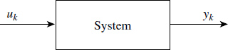
Figure 2.1 A single-input single-output system
sequence uk could be finite while yk could be infinite, which is common. For the system to be linear,
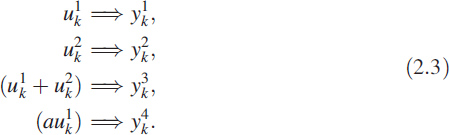
Thus, we must have ![]() and
and ![]() , where a is an arbitrary constant.
, where a is an arbitrary constant.
Consider two cascaded linear systems A and B with input uk and output yk. Linearity demands that exchanging systems will not alter the output for the same input. This is indicated in Figure 2.2.
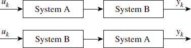
Figure 2.2 Commutative property
2.1.2 Sinusoidal Inputs
Under steady state, linear systems display wonderful properties for sinusoidal inputs. If uk = cos(2πfk) then the output is also a sinusoidal signal given as yk = A cos(2πfk + ϕ). This output also can be written as ![]() , where
, where ![]() and
and ![]() . Mathematicians represent the sequence yk as a complex sequence
. Mathematicians represent the sequence yk as a complex sequence ![]() , where
, where ![]() . Engineers treat yk as an ordered pair of sequences, popularly known as in-phase and quadrature sequences. Note that there is no change in frequency but only change in amplitude and phase. This concept is used in many practical systems, such as network analysers, spectrum analysers and transfer function analysers.
. Engineers treat yk as an ordered pair of sequences, popularly known as in-phase and quadrature sequences. Note that there is no change in frequency but only change in amplitude and phase. This concept is used in many practical systems, such as network analysers, spectrum analysers and transfer function analysers.
2.1.3 Stability
Another important property defining the system is its stability. By definition if uk = δk and the corresponding output is yk = hk, and if the sequence hk is convergent, then the system is stable. Here δk is the unit sample.1 We can also define a summation ![]() and if S is finite, then the system is stable. The physical meaning is that the area under the discrete curve hk must be finite. There are many methods available for testing convergence. One popular test is known as the ratio test, which states that if |hk+1/hk| < 1, then the sequence hk is convergent, hence the system is stable.
and if S is finite, then the system is stable. The physical meaning is that the area under the discrete curve hk must be finite. There are many methods available for testing convergence. One popular test is known as the ratio test, which states that if |hk+1/hk| < 1, then the sequence hk is convergent, hence the system is stable.
2.1.4 Shift Invariance
Shift invariance is another important desirable property. A shift in the input results in an equal shift in the output ![]() . This property is known as shift invariance. Linear and shift invariant (LSI) systems have very interesting properties and are mathematically tractable. This is the reason why many theoretical derivations assume this property.
. This property is known as shift invariance. Linear and shift invariant (LSI) systems have very interesting properties and are mathematically tractable. This is the reason why many theoretical derivations assume this property.
2.1.5 Impulse Response
If the input uk is a unit sample δk, then the system response yk is called a unit sample response of the system, hk. This has a special significance and completely characterises the system. This sequence could be finite or infinite. The sequence hk is said to be finite if
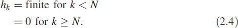
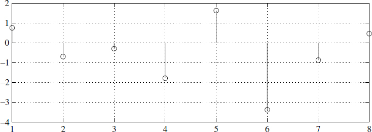
If the impulse response hk is finite as defined in (2.4), then the system is a finite impulse response (FIR) system and it has a special significance. Figure 2.3 shows a typical unit sample response of a system defined by (2.13) and the unit sample response for this system is infinite. Traditionally, systems in the discrete domain originate from differential equations describing a given system, and these differential equations take the form of difference equations in the discrete domain.
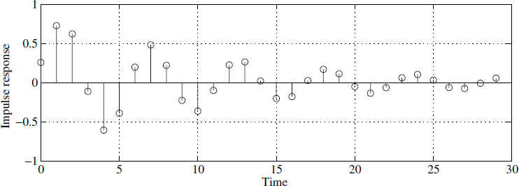
Figure 2.3 Impulse response hk
2.1.5.1 Convolution: Response to a Sequence
Consider a system defined by its unit sample response hk, and let the input sequence be uk of length N. Then the response due to u1 can be obtained using the scaling property as u1hk, and the response due to u2, u3, u4,…, uN+1 can be obtained using the scaling and shifting properties as
![]()
Now, using superposition we obtain the response due to the sequence uk by summing all the terms as
![]()
We need to remember that the term {u1hk} is a sequence obtained by multiplying a scalar u1 with another sequence hk. This mental picture is a must for better understanding the operations below. We obtain the response yk through a familiar operation known as convolution:2
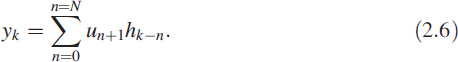
While deriving (2.6) we have used shift invariance properties. The above convolution operation is represented symbolically as yk = uk ⊗ hk. The binary operator ⊗ which represents convolution is linear and follows all the associative and commutative properties. In the frequency domain, convolution takes the form of multiplication, Y(jω) = U(jω) × H(jω), where all the jω functions are corresponding frequency domain functions.
Convolution is also known as filtering and it is also equivalent to multiplying two polynomials, H(z) × U(z). If we have a sequence hk of length m and a sequence uk of length N, then we can see that the output sequence is of size m + N.
Consider the computational complexity of (2.6). Computing u1hk needs m multiplications and m additions. Assuming there is not much difference between addition and multiplication, in the floating-point domain, the computational burden is 2m operations for one term, and the whole of (2.6) requires (2m × N + N − 1) operations. For N = 100, m = 50, which are typical values, we need to perform 10 099 operations. As an engineering approximation, we can estimate this as 2mN operations.
Computing the convolution of two sequences using (2.6) is computationally expensive. Less expensive methods are available based on discrete Fourier transforms (DFTs). This is because there are fast methods for computing DFTs.
2.1.5.2 Autocorrelation Function
Another important operation between two sequences, say uk and hk, is correlation. Typically uk is an input sequence to a linear system and hk is the impulse response of the same system. The correlation function is defined as
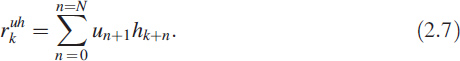
This is also written using the convolution operator as ![]() , where
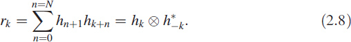
, where ![]() is the conjugate symmetric part of hk. When both sequences in (2.7) are the same and equal to the impulse response hk then
is the conjugate symmetric part of hk. When both sequences in (2.7) are the same and equal to the impulse response hk then ![]() becomes the autocorrelation3 function rk of the system, shown in Figure 2.4(a). The autocorrelation function rk has special significance in linear systems and is given as
becomes the autocorrelation3 function rk of the system, shown in Figure 2.4(a). The autocorrelation function rk has special significance in linear systems and is given as
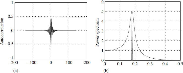
Figure 2.4 Relation between autocorrelation rk and power spectrum ||H(jω)||
The DFT of rk results in the power spectrum of the system. The DFT of the given autocorrelation function rk of a linear system is shown in Figure 2.4(b). Note that rk of a linear system and its power spectrum |H(ejω)| are synonymous and can be used interchangeably. In fact, the Wiener–Khinchin theorem states the same.
2.1.6 Decomposing hk
The impulse response of a given linear system can be considered as a sum of impulse responses of groups of first- and second-order systems. This is because the system transfer function H(z) = B(z)/A(z) can be decomposed into partial fractions of first order (complex or real) or a sum of partial fractions of all-real second-order and first-order systems. This results in the given impulse response hk being expressed as a sum of impulse responses of several basic responses:
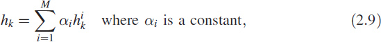
where ![]() is the unit sample response of either a first-order system or a second-order system.
is the unit sample response of either a first-order system or a second-order system.
2.2 Linear System Representation
We would like to avoid continuous systems in this textbook, but we are compelled to mention them, although this is probably the last time. Consider the popular second-order system
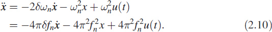
Here
Taking numerical δ = 0.1 and fn = 100 Hz we get
![]()
2.2.1 Continuous to Discrete
Let us take a numerical method [5] known as the Tustin approximation for sampling times of 0.001 s and 0.002 s and apply it to the continuous system characterised by (2.11). We get the difference equations as
![]()
![]()
Note that we have two different difference equations representing the same physical system; this is due to a change in sampling rate. Equation (2.13) has two components: an autoregressive (feedback) component and a moving-average (feedforward) component. By using the notation yk−1 = z−1yk, we define vectors yz and uz:
![]()
And we define the coefficient vectors as
![]()
Using this notation, we write (2.13) in vector form as atyz[yk] = btuz[uk]. In this textbook the delay operator z−1 and the complex variable z−1 have been used interchangeably. We continue to do this even though mathematicians may object. We believe that algebraically there is no loss of generality.
2.2.2 Nomenclature
For historical reasons, specialists from different backgrounds have different names for (2.14) and (2.15). However, they are identical in a strict mathematical sense.
Statisticians use the term Autoregressive (AR) [6]; control engineers call it an all-pole system; and communication engineers call it an infinite impulse response (IIR) filters. The statisticians' moving-average (MA) process is called a feedforward system by control engineers and a finite impulse response (FIR) filter by communication engineers so we have chosen names to suit the context of this textbook; readers may choose other names to suit their own contexts.
2.2.3 Difference Equations
We can write (2.12) or (2.13) in the form
![]()
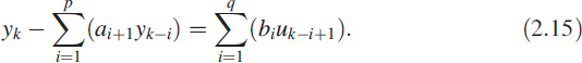
In (2.15) the coefficient a1 is always one. Equations (2.14) and (2.15) are the generic linear difference equations of a pth order AR process (left-hand side) and a qth order MA process (right-hand side). There are many technical names for (2.14) and (2.15).
2.2.4 Transfer Function
Recognising (2.14) as the dot product of the vectors, it can be written as
![]()
where B(z) is called the numerator polynomial and A(z) is called the denominator polynomial. We can recast the equations as yk = [B(z)/A(z)]uk. The roots of B(z) and A(z) have greater significance in the theory of digital filters, and for understanding physical systems and their behaviour. The impulse response of the system (2.13) is depicted in Figure 2.3; it is real. It is not necessary that the response be a single sequence; it could be an ordered pair of sequences, making it complex. We can write B(z)/A(z) as

The same information is shown in Figure 2.5 as a pole-zero plot. We can decompose it into partial fractions as
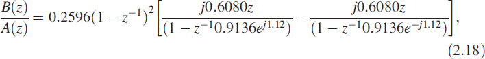
as stated in (2.9). However, it is a recommended practice to leave it as a second-order function if the roots are complex. Second-order systems have great significance and the standard representation is given below, where r = 0.9136 is the radial pole position at an angle of θ = ±1.12 radians in the z-plane.

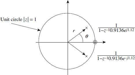
Figure 2.5 Polar plot of the second-order system in (2.17)
2.2.5 Pole–Zero Representation
The polynomials A(z) and B(z) are set equal to zero and solved for z. The roots of the numerator polynomial are called zeros and the roots of the denominator polynomial are called poles of the system. Note that the continuous system represented by (2.10) is defined by only two parameters [δ, ωn] but by converting into discrete form we get three parameters [0.2596, 0.9136, 1.12], as shown in (2.17) and (2.19). The addition of a third parameter is due to the sampling time Ts. The parameter δ represents damping and ω represents the natural angular frequency; they roughly translate into the radial position of the pole and the angular position of the pole, respectively.
2.2.6 Continuous to Discrete Domain
Converting from the continuous domain to the discrete domain also affects the pole positions due to sampling rate. Figure 2.6 depicts the pole positions (r, θ) for various values of δ in the range 0.05 < δ < 0.9 and for different sampling times. We can use Figure 2.6 to make a number of inferences. In this figure we have shown sampling time as 0 to 1; 0 corresponds to an infinite sampling rate whereas 1 corresponds to the Nyquist sampling rate (twice the maximum frequency). The damping factor δ has been varied in the same range for Figure 2.6(a) and (b). A quick look at Figure 2.6(b) shows that the pole angle is insensitive to variations of δ.
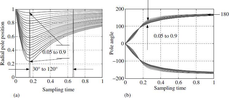
Figure 2.6 Continuous to discrete sensitivities of the system in (2.11)
Time has an approximately linear relation with pole angle θ. Taking advantage of this relation, we have positioned two markers in Figure 2.6(a) at 30° and 120°, which correspond to 12 samples/cycle and 3 samples/cycle, respectively. The pole plot in Figure 2.6(a) shows that the difference equation numerically behaves well in this window.
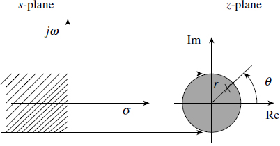
Figure 2.6A Comparing the s-plane with the z-plane
In discrete systems, roots are presented in polar form rather than rectangular form. This is because the s-plane, which represents the continuous domain, is partitioned into a left half and a right half by the jω axis running from ∞ to −∞ (Figure 2.6A). Such an infinite axis is folded into the sum of an infinite number of circles of unit radius in the z-plane, which is the representation in the discrete domain. The top half of the circle (0 to −π) represents DC to Nyquist frequency and the bottom half (0 to π) represents the negative frequencies.
In fact, periodicity and conjugate symmetry properties can be best understood by this geometric background. If all the poles and zeros lie within the unit circle, the system is called a minimum phase system. For good stability, all poles must be inside the unit circle.
2.2.7 State Space Representation
Let us consider (2.14) again. We can write it as yk = [B(z)/A(z)]uk. Using the linearity property, we can write yk = B(z)(wk) where wk = [1/A(z)](uk). Then
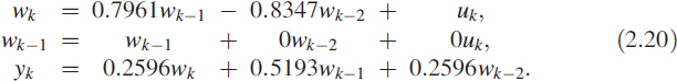
We can modify the last equation in (2.20) as

Now the modified set is
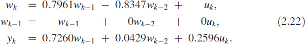
This can be represented in standard A, B, C, D matrix form as


The above difference equation is shown in Figure 2.7, which gives the minimum delay realisation. In brief, wk = Awk−1 + Buk and yk = Ctwk−1 + Duk.

Figure 2.7 Digital filter minimum delay realisation
2.2.8 Solution of Linear Difference Equations
There are many methods available for solving difference equations along the lines of differential equations, by solving for complementary function and particular integral. The advent of powerful software packages such as MATLAB and SIMULINK means that we no longer need to know the details, but if we do understand them, it will help us get the most out of our software.
It is always better to visualise the systems in the form of (2.16) since this best matches the software packages in the commercial market. The transfer function H(z) = B(z)/A(z) can be converted into a sum of second- and/or first-order partial fractions, depending on whether the roots of the polynomial A(z) are real or complex:

A second-order system has a solution of the form hk = Ar−k cos(θ) + Br−k sin(θ), whereas a first-order system is of the form hk = Cr−k; the constants can be evaluated from the initial conditions. Equations (2.25) and (2.9) are the same except the domains are different. The overall solution for a specific input uk can be obtained using (2.6).
2.3 Random Variables
We will introduce two important ideas:
- Continuous random variable (CRV)
- Discrete random variable (DRV)
Note that not every discrete system is a DRV; discrete systems and discrete random variables are separate concepts. Sampling or converting into a discrete signal show its effect on the autocorrelation function rk but not on its probability density function fx(x). For completeness, we recollect that a random variable (rv) is a function mapping from a sample space to the real line.
Consider a roulette wheel commonly used in casinos. The sample space is {0 ≤ θ ≤ 2π} and the function is θ = 1/2π. In the case of a CRV, suppose we ask, What is the probability θ = 20°. The spontaneous answer would be zero. But if we want P(10° ≤ θ ≤ 20°), then it is 1 /36. The idea of presenting a CRV this way is to illustrate the continuous nature of its pdf.
Consider another experiment of throwing a die or picking a card from a pack of 52. This is a DRV experiment for the simple reason that the sample space is finite and discrete. The pdf is discrete and exists only where an event occurs. If the earlier roulette wheel is mechanically redesigned so it will stop only at θ = {0°, 1°, 2°,…, 359°}, then θ becomes a DRV.
2.3.1 Functions of a Random Variable
Let us examine a few important relationships between functions of random variables. Most of the noise propagation in linear systems can be best understood by applying these golden rules partially or in full:
- Consider a simple relation z = x + y, then the pdf of z is obtained by convolving the pdf of x and y, fz(z) = fx(x) ⊗ fy(y).
- For the relation y = mx + c, the pdf of y is
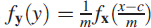 .
. - The central limit theorem says that if xi is a random variable of any distribution, then the random variable y defined as
 has a normal distribution, where N is a large number. As an engineering approximation, N ≥ 12 will suffice.
2.3.1.1 Hit Distance of a Projectile
This problem comes under non-linear functions of a random variable. To illustrate the idea, consider a ballistic object moving under the gravitational field shown in Figure 2.8 with a gravitational constant g = 9.81 m/s2:
![]()
![]()
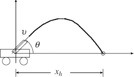
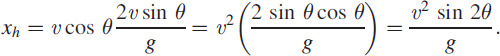
Setting y = 0 we get t = (2υ/g) sinθ for t ≠ 0, then the horizontal distance where it hits the ground is
Consider υ as statistically varying with μυ = 50 and συ = 0.2 and μθ = π/3 and σθ = π/30 We have derived a closed-form solution (Figure 2.9) for the above pdf in the interval 85 < x < 250:

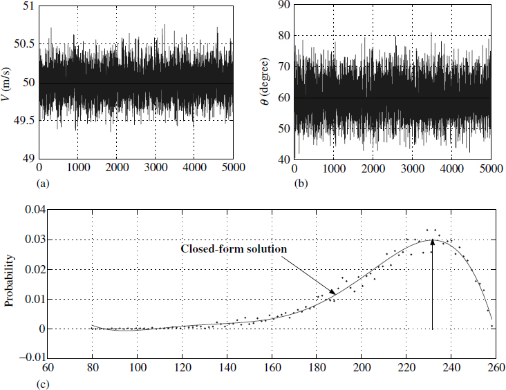
Figure 2.9 Functions of random variables
In this case we could find out the desired pdf but it is only because we have a closed-form solution for xh as (υ2/g)sin 2 θ.
2.3.2 Reliability of Systems
Systems are designed from components having different failure probabilities. A complex system is a function of many random variables and the study of these interconnected subsystems constitute an important branch of engineering. This must always be borne in mind by every product designer and practising engineer. Reliability can be achieved only at the product design stage, not at the end, hence product designers should pay attention to reliability.
In the case of software, system failures occur due to existence of many paths due to different input conditions and it behaves as a finite-state automaton. It is almost impossible to exhaust all the outcomes for all conditions. In fact, this is why many practices have been introduced in testing at each level. Reliability of the software improves with use whereas the reliability of a mechanical system degrades with use. Figure 2.10 shows the reliability graph of any generic system. Notice there are three phases in the graph: infantile mortality, random failures and aging. In the case of software there are only two phases exist; the aging phase doesn't exist.
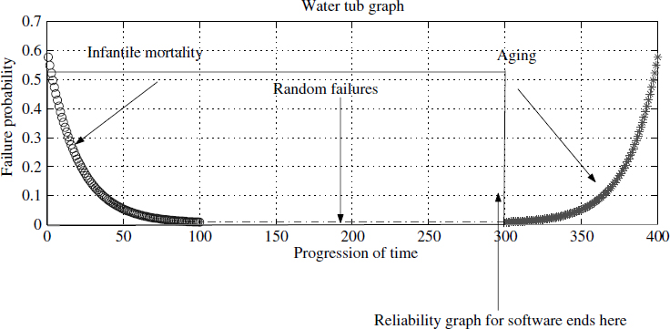
Figure 2.10 System reliability is a function of random variables
2.4 Noise
All textbooks of communication engineering and books on other disciplines define noise as an unwanted signal. Noise is characterised by two parameters: its amplitude statistics (probability density function) and its autocorrelation function rk. Both of them are important and independent.
2.4.1 Noise Generation
On many occasions we need to generate specific types of noise. The most frequently used noise is white Gaussian noise (WGN). We cannot appreciate any noise in the time domain. The only way to get some information is by constructing the pdf of the given signal. There are many methods for generating WGN. The primary source is a uniformly distributed noise (UDN), which can be generated using a linear congruential generator (LCG), well explained by Knuth [10]. Figure 2.11 depicts the LCG relation given as μk = (aμk−1 + c) mod m, where the constants a and c can be chosen to suit the purpose.
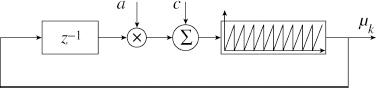
Figure 2.11 Linear congruential generator for UDF
WGN is generated by invoking the central limit theorem and also recollecting that the variance of UDN is A2/12. Now WGN γk is given as ![]() . Choosing 12 in the summation cancels the denominator 12 in the UDN μk.
. Choosing 12 in the summation cancels the denominator 12 in the UDN μk.
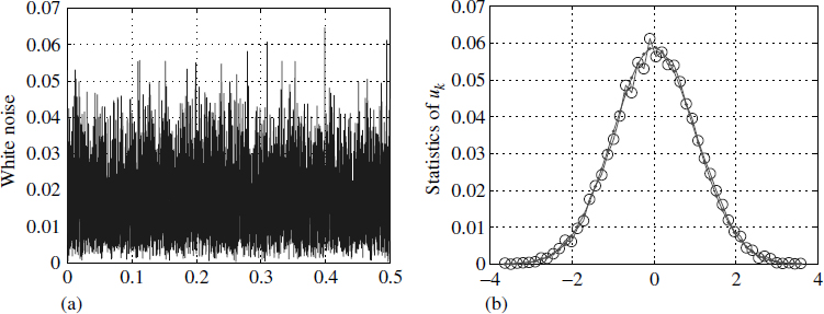
Figure 2.12 Amplitude statistics of uk
2.4.2 Fourier Transform and pdf of Noise
We have constructed the pdf of a noise signal uk that is white and Gaussian. It is given in Figure 2.12 for a WGN.
If the autocorrelation function rk = δk, then the noise is white. This is because the power spectrum of the noise is flat or the power level at all frequencies is constant. This whiteness (Figure 2.12(a)) is independent from the pdf of the noise (Figure 2.12(b)). The implication of this statement is that the pdf can be of any form. When the amplitude statistics of the given time series have a Gaussian distribution, and the power spectrum of the same signal has power levels constant and uniform across all the frequencies, then it is called white Gaussian noise, which essentially means that rk = δk.
2.5 Propagation of Noise in Linear Systems
When a WGN (Figure 2.12) is passed through a filter, the output is a coloured noise as in Figure 2.13(a). Here the amplitude statistics continue to remain Gaussian, as in Figure 2.13(b).
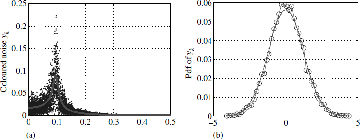
Figure 2.13 Amplitude statistics and power spectrum of yk
Coloured Gaussian noise has identical structure or shape to the input (uk) amplitude statistics, as in Figure 2.12(b). The output is said to be coloured, because spectral energy is not constant across all the frequencies, as shown in Figure 2.13(a)
Taking linear systems having either an IIR or an FIR and exciting them with Gaussian noise results in another Gaussian noise of different mean and variance. This is an important characteristic exhibited by linear systems and is illustrated in Figures 2.12 and 2.13. In this context, it is worth recollecting that a sine wave input to a linear system results in another sine wave with the same frequency but different amplitude and phase.
2.5.1 Linear System Driven by Arbitrary Noise
Consider an AR system defined by (2.23) and (2.24) and where the input uk is uncorrelated and stationary. The output of this system is normal. As an example, let us excite the system with uk having a Weibull distribution as in Figure 2.14 with α = 0.1 and β = 0.8:
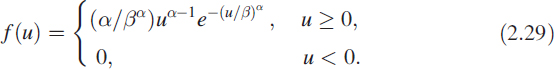
The output is normal, as shown in Figure 2.14. This can be understood by realising that the output can be best approximated using an MA process as in (2.5) and (2.6) and that the statistics of uk are the same as the statistics of uk+i. Then use the three rules in Section 2.3.1 to obtain the output as a normal distribution.
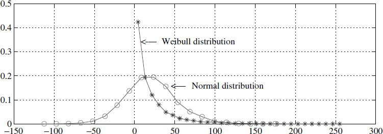
Figure 2.14 Input and output statistics of uk and yk
2.6 Multivariate Functions
Understanding functions of several variables is important for estimating parameters of systems. Often the problem is stated like this: Given a system, find out its response to various inputs. This is a fairly simple problem known as synthesis. Given the input and output, finding the system is more difficult; plenty of methods are available and they depend on the specific nature of the problem. This section tries to lay foundations for understanding parameters in more than one or two dimensions.
It is the limitation of the mind that makes it difficult to perceive variables beyond three dimensions. Even a school student can understand two dimensions with ease. A point in the Cartesian frame is represented by an ordered pair with reference to x1 and x2 axes, which are orthogonal to each other (Figure 2.15). Our mind is so well trained it can understand and perceive all the concepts in two dimensions. The difficulty comes once we go beyond two dimensions, and this puts the mind under strain.
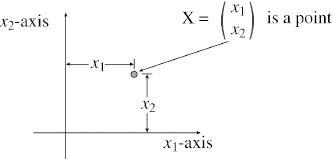
Figure 2.15 Two-dimensional representation
2.6.1 Vectors of More Than Two Dimensions
This section presents a novel way of visualising multidimensional variables. The traditional approach is to imagine a hyperspace and treat it as a point. But we will present a simple way of looking at the multidimensional vector, yet without losing any generality. Consider a four-dimensional vector. xt = [x1, x2, x3, x4] has been represented as a polygon of 5 sides in Figure 2.16. This provides more insight into understanding parameters of many dimensions. A multidimensional vector is a figure but not a point. Visualising an n-dimensional vector as a polygon of order n + 1 is an important aspect of understanding multivariate systems. This shows how difficult it is to compare two figures or perform any standard binary operations on them. Many times we need to find out maxima or minima in this domain. This will help us to understand these concepts better. Comparing numbers or performing the familiar binary operations such as +, −, ÷, × is easy but it is more difficult with multidimensional vectors as they are polygons. It doesn't mean that we cannot compare two polygons; there are methods for doing this.
2.6.2 Functions of Several Variables
Multivariate functions are so common in reality, we cannot avoid handling them. They could be representing a weather system or a digital filter; the motion parameters of a space shuttle, a missile or an aircraft; the performance of a person or company; the financial stability of a bank; and so on. The problem is to compare these multivariate functions by making judgements about their maxima or minima. In this context, understanding the n-dimensional vector gives a better solution to the problems. Control engineers and statisticians [7] have used these functions extensively.
Figure 2.16 Representing a multidimensional vector
Consider a multivariate function yk = f(xk, uk) where xk is a multidimensional vector and u is the input. This function describes a system. There are many times we need to drive the given system in a specific trajectory in a multidimensional space, subject to some conditions.
A digital filter defined in (2.23) and (2.24) is the best example of such functions and is written like this:
![]()
2.6.3 System of Equations
Another example of a multivariate function is a system of simultaneous equations. For the sake of brevity and comprehension, let us consider the following equations. Equations of this type are encountered in different ways in many applications. Pay attention to this subsection and it will give you a good insight into many solutions.
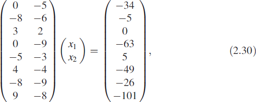
![]()
Equation (2.31) is a concise matrix way of representing the system of equations given in (2.30). In this particular case, matrix A is 8 × 2. The inverse of a matrix is defined only when A is square and |A| ≠ 0. A very innovative approach was adapted by Moore and Penrose for inverting a rectangular matrix.
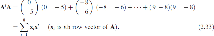
Take (2.31) and premultiply by At to obtain
![]()
The matrix AtA is square and can also be written as4
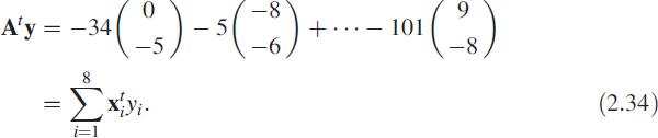
The column vector Aty can be written as
Under the assumption that AtA is non-singular, the inverse can be obtained recursively or en block. Then the solution for the system (2.30) is given as
![]()
where ![]() is known as the Moore–Penrose pseudo-inverse [1,8]. The solution is x = A+y. There are two ways of looking at it. One way is that it corresponds to the best intersection [9] of all the intersections in Figure 2.17, in a least-squares sense. The other way is that the rows of A+ corresponds to MA processes or FIR filters. Figure 2.18 depicts the error ek (in simple language it is the deviation from the straight line fit). Sometimes ∈k is called an innovation process [4] and is given as ek = AA+y − y (Figure 2.18).
is known as the Moore–Penrose pseudo-inverse [1,8]. The solution is x = A+y. There are two ways of looking at it. One way is that it corresponds to the best intersection [9] of all the intersections in Figure 2.17, in a least-squares sense. The other way is that the rows of A+ corresponds to MA processes or FIR filters. Figure 2.18 depicts the error ek (in simple language it is the deviation from the straight line fit). Sometimes ∈k is called an innovation process [4] and is given as ek = AA+y − y (Figure 2.18).
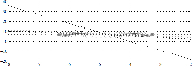
Figure 2.17 A system of linear equations
2.7 Number Systems
A good understanding of binary number systems provide a proper insight into digital filters and their implementations. Consider a binary number bn = xnxn−1… x3x2x1, where the symbol xi, called a bit of the word bn, takes value 0 or 1. The string of binary symbols has a value given as
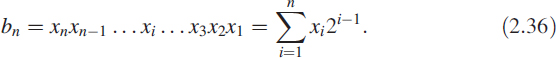
This representation is an unsigned representation of integer numbers. For a given value of n we can generate 2n − 1 patterns. If we fix the value n, normally known as word length, to accommodate the positive and negative numbers, the usable numbers gets partitioned into half each. There are three common ways of doing it. For illustration we choose the value n = 3.
2.7.1 Representation of Numbers
2.7.1.1 Sign Magnitude Form
Let us consider a set of 8 numbers {0, 1, 2, 3, 4, 5, 6, 7} representing a 3-bit binary numbers and mapped as {+0, +1, +2, +3, −0, −1, −2, −3}. Here we have divided the given set into two partitions of positive numbers and negative numbers. Human beings understand decimal numbers the best, so we are trying to explain with equivalent decimal numbers whose binary bit patterns are the same. The basic problem is that the hardware is relatively complex and the non-uniqueness of +0 and −0 is not acceptable in the mathematical sense. Sign magnitude form is abbreviated to SM.
2.7.1.2 Ones Complement Form
In ones complement form (1sC) the same numbers {0, 1, 2, 3, 4, 5, 6, 7} are designated as {+0, +1, +2, +3, −3, −2, −1, −0}. This method is relatively easy to implement but still has the problem of a non-unique zero.
2.7.1.3 Twos Complement Form
Twos complement form (2sC) is the most popular numbering and is practised widely in all machines. In this scheme the positive zero and negative zero are removed and the numbers {0, 1, 2, 3, 4, 5, 6, 7} are mapped as {0, 1, 2, 3, −4, −3, −2, −1}.
2.7.1.4 The Three Forms in a Nutshell
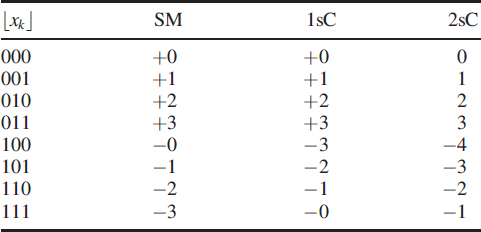
Table 2.1 illustrates the three representations in a nutshell. Sign magnitude is very popular in A/D converters and it is almost a standard practice in all arithmetics to use a twos complement number system.
Table 2.1 The three representations in a nutshell
2.7.2 Fixed-Point Numbers
Similar to the imaginary decimal point, we have a binary point that can be positioned anywhere in the binary number bn (2.36) and can be written as
![]()
Now the value of bn takes the form of a rational number bn/2n−1; all other things remain the same. It could be SM, 1sC or 2sC. The above form is called the normalised form. It essentially imposes a restriction that it is permitted to have only one bit to the left of the imaginary binary point
2.7.3 Floating-Point Numbers
Fixed-point representation suffers from the limitation of dynamic range, hence the floating point has evolved to give
![]()
where m is the mantissa and c is the characteristic or exponent; xn is the sign bit. The floating-point number is represented as a 3-tuple given as bn = {xn, m, c} in packed form. The standard5 IEEE format for 32-bit single-precision floating-point number is given as
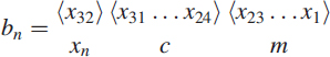
In this notation, m is a fixed-point positive fractional number in normalised form and the value bn represented by the word may be determined as follows:
- If 0 < c < 255 then bn = −1xn × 2c−127 × (1.m) where 1.m is intended to represent the binary number created by prefixing m with an implicit leading 1 and a binary point.
- If c = 0 and m ≠ 0, then bn = −1xn × 2−126 × 0.m These are unnormalised values.
- If c = 255 and m ≠ 0, then bn = NaN (Nan means not a number).
- If c = 255 and m = 0 and xn = 1 or 0, then bn = −∞ or bn = ∞.
- If c = 0 and m = 0 and xn = 1 or 0, then bn = −0 or +0
2.8 Summary
This chapter was a refresher on some relevant engineering topics. It should help you with the rest of the book. We considered the autocorrelation function, representation of linear systems, and noise and its propagation in linear systems. We also discussed the need to know about systems reliability. Most problems in real life are inverse problems, so we introduced the Moore–Penrose pseudo-inverse. We concluded by providing an insight into binary number systems.
References
1. S. Slott and L. James, Parametric Estimation as an Optimisation Problem. Hatfield Polytechnic.
2. D. G. Luenberger, Introduction to Linear and Non-linear Programming. Reading MA: Addison-Wesley, 1973.
3. T. L. Boullion and P. L. Odell, Generalised Inverse Matrices. New York: John Wiley & Sons, Inc., 1971.
4. A. V. Openheim, A. S. Wilsky and I. T. Young, Signals and Systems. Englewood Cliffs NJ: Prentice Hall, 1983.
5. R. Isermann, Digital Control Systems. Berlin: Springer-Verlag, 1981.
6. J. R. Wolberg, Prediction Analysis. New York: Van Nostrand, 1967.
7. S. Brandt, Statistical and Computational Methods in Data Analysis. Dordrecht: North Holland, 1978.
8. A. Albert, Regression and the Moore–Penrose Pseudoinverse. New York: Academic Press, 1972.
9. P. Lancaster, The Theory of matrices: With Applications, 2nd edn.
10. Donald E. Knuth, Art of Computer Programming.
Digital Signal Processing: A Practitioner's Approach K. V. Rangarao and R. K. Mallik
© 2005 John Wiley & Sons, Ltd
1Impulse response is used in continous systems.
4This is useful in inverting recursively using a matrix inversion lemma which states that ![]() .
.
5ANSI/IEEE Standard 754-1985, Standard for Binary Floating Point Arithmetic.