6

Case Studies

Digital signal processing is all-pervading, so we have mostly selected the areas that interest engineers. Often the solutions look very similar, indicating many commonalities between them. These case studies also demonstrate that it is very difficult to categorise a given problem as exclusively DSP or non-DSP. Frequently we need to stretch our engineering hand a little and remove our blinkers to get an overall view of the solution.

In addition, problems are non-linear and we need a good systems background as well as DSP. Inverse problems are more difficult than forward problems or synthesis. For instance, the design of a filter for a given specification is trivial. It is the combinations of many disciplines put together that makes a problem very interesting. Perhaps you feel that problems are centred around some common solutions. But this chapter aims to demonstrate that the essence of any solution is a good problem formulation.

6.1 Difference Equation to Program

The following C code is for a digital filter implementation that includes testing by exciting it with a white Gaussian noise (WGN); the output is captured in the file fiiter.dat. The spectral characteristic of the output time series is the same as that of the filter, since the input is a WGN. This code demonstrates only that converting a given difference equation to a code is relatively trivial. Here we designate xk1 = x_k, xk2 = x_k−1, xk3 = x_k−2 and the filter is x_k = 0.5871 x_k−1 − 0.9025* x_k−2 + 0.0488 * (u_k − u_k−2).

// Translating a difference equation to C


# include <stdio.h>
# include <stdlib.h>

# include <math.h>

float randn(void); FILE *fp_write;
void main (void)
{
int k,kmax=5000;
float pi,yk,f=0.1;float xk1=0.0,xk2=0.0, xk3=0.0;
float uk1 = 0.0,uk2=0.0, uk3=0.0;
fp_write = fopen(“filter.dat”, “w”);
pi = (atan(1.0))*4.0; randomise();
printf(“ start 
”);
         for (k=0; k < kmax; k++)
                {
                  uk1=randn(); xk3=xk2; xk2=xk1;
                  uk3=uk2; uk2=uk1;
      xk1 = 0.5871*xk2 − 0.9025*xk3 + 0.0488* (uk1−uk3);
                  fprintf(fp_write,“%d %f 
”, k, xk1);
                }
printf(“ finish 
”);
fclose(fp_write);
}

The following program generates white Gaussian noise by adding 12 uniformly distributed random variables.

float randn(void)
{
float intmax,udf,sum;
int rnd,k;


intmax = RAND_MAX;
       sum = 0.0;
       for (k=0; k < 12; k++)
       {
         rnd = rand(); udf = rnd;
         udf = (udf/intmax)−0.5; sum = sum + udf;
       }
return(sum);
}

6.2 Estimating Direction of Arrival

Estimating direction of arrival (DoA) is of continual interest to people working on underwater systems or RF systems. Locating a radiating source [1, 6, 7] requires us to determine the DoA of energy from a mobile phone, a push-to-talk or an underwater acoustic emitter. Monopulse radar [5] also works on the same principle, as shown below.

To understand this in simple terms, let us consider three directional receivers as shown in Figure 6.1. Each directional receiver consists of a set of antenna elements and a receiver that has a definite gain pattern. The first receiver provides an output r₁ in a given direction θ. To be more precise, we assume an emitter of a given power when moved at a constant distance. Put another way, in a circle around this directional receiver, the output r₁ follows the pattern in Figure 6.1.

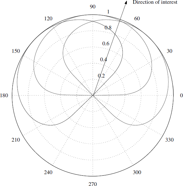
Figure 6.1 Directional receivers r = | sinθ|^0.25 for θ = 0 to π

When we have three such receivers each shifted by 45° we get a response vector , where each element represents the response of each receiver. Now we map this 3-tuple Θ to a scalar θ. Let the ensemble of vectors be A = [Θ₁ Θ₂… Θ_N]. We can see that A is an N × 3 matrix in this case. This data is generated at the design time and needs to be obtained at periodic intervals. Let Φ be a vector obtained at a given time, then we define a function . Using this we generate another function .

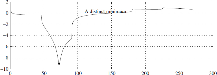
Figure 6.2 Minima in the direction of the emitter

This is plotted and shown in Figure 6.2, which has a distinct minimum representing the direction of the radiating source. Numerically locating this minimum gives the direction of the emitter.

6.3 Electronic Rotating Elements

In the previous section we saw that the phase delay φ between two elements can be modulated by rotating one element around the other. The rotation need not be done mechanically. To see how the rotating measuring system works, consider 12 elements positioned around a centre element (Figure 6.3). The delay at the ith element is

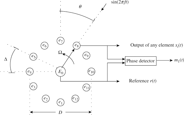
Figure 6.3 Finding direction with rotating elements

where is the projected element distance and Ω is the angular rotation of the elements.

The phase detector output m₁(t) is obtained from r(t) = sin(2πft) and x_i(t):

Signal m₁(t) is passed through an FM discriminator and another phase detector, giving

where A_x = K_x cos(θ), A_y = K_y sin(θ) and e = K_x − K_y is zero in a least-squares sense for a given system. Traditional analogue systems present DoA by inputting (t) and (t) to an X–Y scope, shown in Figure 6.4(a). The phase distortions ψ₁(t) and ψ₂(t) are the undesired phase modulations due to multiple reflections, instrumentation errors, etc., and the plot between (t) and (t) results in a distorted figure of eight. The ratio between the amplitudes of (t) and (t) has the DoA information in it and the sinusoids are in phase with each other. However, finding a direct ratio is catastrophic and here we formulate it as a DSP problem.

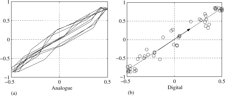
Figure 6.4 DOA using DSP in a rotary system

6.3.1 Problem Formulation

The two signals (t) and (t) are converted to the digital domain as

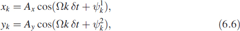
where δt is the sampling time.

6.3.2 Finding DoA

The prime objective here is to estimate the DoA (θ) and the quality of the DoA from the digitised signals x_k and y_k of N samples. The principle of the method is to plot x_k, y_k values in a 2D space and to find a best-fit straight line using linear regression. The slope of this line gives tan(DoA), from which we compute DoA. The mean square error is calculated and is used as a measure of the quality of the DoA given by the system. This is shown in Figure 6.4(b) and the theory is elaborated below.

6.3.3 Straight-Line Fit

The general equation for a straight line can be written as

where m = p₁ and c = p₂ are the slope and the abscissa of the straight line, respectively. Let

We formulate an N × 2 rectangular matrix A given as

Then we write the set of equations (6.8) in matrix form:

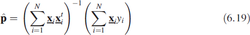
Finding a best-fit straight line involves estimating p from the given A and y. Premultiplying (6.15) by A^t, we get

Here (A^tA) is a 2 × 2 matrix and if its inverse exists, we can write

where is the estimate of p corresponding to the best-fit straight line and A⁺ is known as the Moore–Penrose pseudo-inverse [1]. Equation (6.18) can be rewritten as

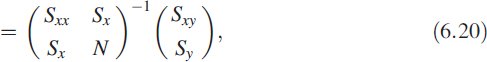
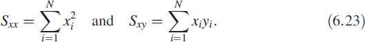
where is defined by (6.12) and the terms S_xx, S_x, S_y, S_xy are defined in (6.22) and (6.23).

But the above solution is computationally intensive as it involves matrix multiplications and a matrix inversion. A recursive solution is available for (6.19) but even though it is not as computationally intensive, it still requires considerable time [2, 3].

6.3.3.1 Closed-Form Solution

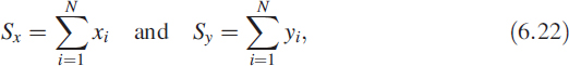
To avoid such time-consuming calculations, a closed-form solution for (6.20) is used [4]. The expressions are

where

Then the sum of squares of errors is given as , where . So

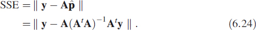
Again, to find the sum of squares of errors, a closed-form solution for (6.24) is used [4] to reduce the computational complexity:

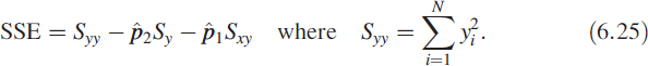
We have illustrated various DSP techniques to improve or extract the hidden data by ingeniously combining ideas from systems engineering. The numbers of interest are , (Figure 6.4) and SSE (6.25).

6.4 Summary

In this chapter we gave a detailed treatment of a specific problem in direction finding, showing the need to understand systems engineering in order to implement DSP algorithms. It is very difficult to isolate DSP problems from other areas of engineering. Practical problems tend to cover many areas but centre on one area that demands the principal focus.

References

1. A. Albert, Regression and the Moore–Penrose Pseudoinverse. New York: Academic Press, 1972.

2. D. M. Himmelblau, Applied Non-linear Programming, p. 75. New York: McGraw-Hill, 1972.

3. D.C. Montgomery et al., Introduction to Linear Regression, Ch. 8. New York: John Wiley & Sons, Inc., 1982.

4. J. L. Devore, Probability and Statistics for Engineers and the Sciences. Monterey CA: Brooks Cole, 1987.

5. D. Curtis Scheler, Introduction to Electronic Warfare, pp. 326–30. Norwood MA: Artech House, 1990.

6. H. H. Jenkins, Small-Aperture Radio Direction Finding, pp. 139–48. Norwood MA: Artech House, 1991.

7. G. Multedo, ‘Direction finding.’ Revue Technique Thomson-CSF, 19(2), 1987.