
Chapter 14. Spreading
14.1. A New Job
We open with a shot of a fishing boat where a father and son work on tempting the fish with seductive offers of worms and minnows.
| Father: | It makes me happy to have my son come home from college and stay with us. |
| Son: | Ah, quit it. |
| Father: | No. Say something intelligent. I want to see what I got for my money. |
| Son: | Quit it. |
| Father: | No. Come on. |
| Son: | The essential language of a text is confusion, distraction, misappropriation, and disguise. Only by deconstructing the textual signifiers, assessing and reassessing the semiotic signposts, and then reconstructing a coherent yet divergent vision can we truly begin to apprehend and perhaps even comprehend the limits of our literary media. |
The son reels in his line and begins to switch the lures.
| Father: | It makes me proud to hear such talk. |
| Son: | I'm just repeating it. |
| Father: | A degree in English literature is something to be proud of. |
| Son: | Well, if you say so. |
| Father: | Now, what are you going to do for a job? |
| Son: | Oh, there aren't many openings for literature majors. A friend works at a publishing house in New York… |
The son trails off, the father pauses, wiggles in his seat, adjusts his line and begins.
| Father: | There's no money in those things. College was college. I spoke to my brother Louie, your uncle, and he agrees with me. We want you to join the family business. |
| Son: | The import/export business? What does literature have to do with that? |
| Father: | We're not technically in import and export. |
| Son: | But. |
| Father: | Yes, that's what the business name says, but as you put it, there's a bit of confusion, distraction and disguise in that text. |
| Son: | But what about the crates of tomatoes and the endless stream of plastic goods? |
| Father: | Subtext. We're really moving money. We specialize in money laundering. |
| Son: | What does money have to do with tomatoes? |
| Father: | Nothing and everything. We move the tomatoes, they pay us for the tomatoes, someone sells the tomatoes, and in the end everyone is happy. But when everything is added up, when all of the arithmetic is done, we've moved more than a million dollars for our friends. They look like tomato kings making a huge profit off of their tomatoes. We get to take a slice for ourselves. |
| Son: | So it's all a front? |
| Father: | It's classier if you think of the tomatoes as a language filled with misdirection, misapprehension, and misunderstanding. We take a clear statement written in the language of money, translate it into millions of tiny tomatoe sentences, and then, through the magic of accounting, return it to the language of cold, hard cash. |
| Son: | It's a new language. |
| Father: | It's an old one. You understand addition. You understand the sum is more than the parts. That's what we do. |
| Son: | So what do you want from me? |
| Father: | You're now an expert on the language of misdirection. That's exactly what we need around the office. |
| Son: | A job? |
| Father: | Yes. We would pay you three times whatever that publishing firm would provide you. |
| Son: | But I would have to forget all of the words I learned in college. I would need to appropriate the language of the stevedores and the longshoremen. |
| Father: | No. We want you to stay the way you are. All of that literature stuff is much more confusing than any code we could ever create. |
Father and son embrace in a happy ending unspoiled by confusion or misdirection.
14.2. Spreading the Information
Many of the algorithms in this book evolved during the modern digital era where bits are bits, zeros are zeros and ones are ones. The tools and the solutions all assume that the information is going to be encoded as streams of binary digits. Tuning the applications to this narrow view of the world is important because binary numbers are the best that the modern machines can do. They are still capable of hair-splitting precision, but they do it by approximating the numbers with a great deal of bits.
The algorithms in this chapter take a slightly different approach. While the information is still encoded as ones or zeros, the theory involves a more continuous style. The information at each location can vary by small amounts that may be fractions like .042 or 1.993. This detail is eventually eliminated by rounding them off, but the theory embraces these fractional values.
This is largely because the algorithms imitate an entire collection of techniques created by radio engineers. Radio engineers attacked a similar problem of hiding information in the past when they developed spread-spectrum radio using largely analog ideas. In the beginning, radios broadcast by pumping power in and out of their antenna at a set frequency. The signal was encoded by changing this power ever so slightly. Amplitude modulated radios (AM) changed the strength of signal while frequency modulated radios (FM) tweaked the speed of the signal a slight amount. To use the radio engineers words, all of the “energy” was concentrated at one frequency.
spread-spectrum radio turned this notion on its head. Instead of using one frequency, it used several. All of the energy was distributed over a large number of frequencies— a feat that managed to make radio communication more secret, more reliable, more efficient and less susceptible to jamming. If the signal lived on many different frequencies, it was much less likely that either intentional or unintentional interference would knock out the signal. Several radios could also share the same group of frequencies without interfering. Well, they might interfere slightly, but a small amount wouldn't disrupt the communications.
Many of the techniques from the spread-spectrum radio world are quite relevant today in digital steganography. The ideas work well if the radio terminology is translated into digital speak. This is not as complicated as it looks. Plus, using digital metaphors can offer a few additional benefits which may be why most spread-spectrum radios today are entirely digital.
The basic approach in radio lingo is to “spread the energy out across the spectrum”. That is, place the signal in a number of different frequencies. In some cases, the radios hop from frequency to frequency very quickly in a system called time sequence. This frequency hopping is very similar to the technique of using a random number generator to choose the locations where the bits should be hidden in a camouflaging file. In some cases, the same random number generators developed to help spread spectrum radios hop from frequency to frequency are used to choose pixels or moments in an audio file.
Sometimes the systems use different frequencies at the same time, an approach known as direct sequence. This spreads out the information over the spectrum by broadcasting some amount of in-formation at one frequency, some at another, etc. The entire message is reassembled by combining all of the information.
The way the energy is parceled out is usually pretty basic. At each instance, the energy being broadcast at all of the frequencies is added up to create the entire signal. This is usually represented mathematically by an integral. Figure 14.1 shows two hypothetical distributions. The top integrates to a positive value, say 100.03, and the bottom integrates to 80.2. Both functions look quite similar. They have the same number of bumps and the same zero values along the x-axis. The top version, however, has a bit more “energy” above the x-axis than the other one. When all of this is added up, the top function is sending a message of “100.03”
Figure 14.1. The energy spread over a number of different frequencies is computed by integration. The top function integrates to say 100.03 and the bottom integrates to 80.2. Both look quite similar but the top one is a bit more top-heavy.

spread-spectrum radio signals like this are said to be resistant to noise and other interference caused by radio jammers. Random noise along the different frequencies may distort the signal, but the changes are likely to cancel out. Radio engineers have sophisticated models of the type of noise corrupting the radio spectrum and they use the models to tune the spread-spectrum algorithms. Noise may increase the signal at one frequency, but it is likely to decrease it somewhere else. When everything is added together in the integral the same result comes out. Figure 14.2 shows the same signals from Figure 14.1 after a bit of noise corrupts them.
Figure 14.2. The signals from Figure 14.1 after being changed by a bit of random noise. The integrals still come out to 100.03 and 80.2.

A radio jammer trying to block the signal faces a difficult challenge. Pumping out random noise at one frequency may disrupt a signal concentrated at that single frequency, but it only obscures one small part of the signal spread out over a number of frequencies. The effects of one powerful signal are easy to filter out by placing limits on the amount of power detected at each frequency.
If a jammer is actually able to identify the band of frequencies used for the entire spread-spectrum signal, it is still hard to disrupt it by injecting random noise everywhere. The noise just cancels out and the signal shines through after integration. In practice, there are ways to jam spread-spectrum signals, but they usually require the jammer to pump out significantly more power. Large amounts of noise can disrupt the system.
These algorithms for spreading information out over a number of bits are very similar to the error-correcting codes described in Chapter 3.
14.3. Going Digital
The spread-spectrum solutions use the analog metaphors of continuous functions measuring “energy” that are evaluated using integration. In the digital world, integers measuring any quantity define discrete functions. In many cases, they measure energy. The integers that define the amount of red, blue and green color at any particular pixel measure the amount of red, green and blue light coming from that location. The integers in a sound file measure the amount of energy traveling as a pressure wave. Of course, the same techniques also work for generic numbers that measure things besides energy. There's no reason why these techniques couldn't be used with an accounting program counting money.
A “spread-spectrum” digital system uses the following steps:
- Choose the Locations If the information is going to be spread out over a number of different locations in the document, then the locations should be chosen with as much care as practical. The simplest solution is choose a block of pixels, a section of an audio file, or perhaps a block of numbers. More complicated solutions may make sense in some cases. There's no reason why the locations can't be rearranged, reordered, or selected as directed by some keyed algorithm. This might be done with a sorting algorithm from Chapter 13 to find the right locations or a random number generator that hops from pixel to pixel finding the right ones.
- Identify the Signal Strength Spread spectrum solutions try to hide the signal in the noise. If the hidden signal is so much larger than the noise that it competes with and overwhelms the main signal, then the game is lost.Choosing the strength for the hidden signal is an art. A strong signal may withstand the effects of inexact compression algorithms but it also could be noticeable. A weaker signal may avoid detection by both a casual user and anyone trying to recover it.
- Study the Human Response Many of the developers of spread-spectrum solutions for audio files or visual files study the limits of the human's senses and try to arrange for their signals to stay beyond these limits. The signal injected into an audio file may stay in the low levels of the noise or it may hide in the echoes.Unfortunately, there is a wide range in human perception. Some people have more sensitive eyes and ears. Everyone can benefit from training. Many spread-spectrum signal designers have developed tools that fooled themselves and their friends, but were easily detected by others.
- Inject the Signal The information is added to the covering data by making changes simultaneously in all of the locations. If the file is a picture, then all of the pixels are changed by a small amount. If it's a sound file, then the sound at each moment gets either a bit stronger or a bit weaker.
The signal is removed after taking the same steps to find the right locations in the file.
Many approaches to spread-spectrum signal hiding use a mathematical algorithm known as the Fast Fourier Transform. This uses a collection of cosine and sine functions to create a model of the underlying data. The model can be tweaked in small ways to hide a signal. These approaches might be said to be everything in parallel. More modern variations use only the cosine (Discrete Cosine Transform), the sine (Discrete Sine Transform), or more complicated waveforms altogether (Discrete Wavelet Transform).
14.3.1. An example
Figure 14.3 shows the graph of .33 seconds from a sound file with samples taken 44,100 times per second. The sound file records the sound intensity with a sequence of 14,976 integers that vary from about 30,000 to about −30, 000. Call these xi, where i ranges between 0 and 14975.
Figure 14.3. A graph of a .33 seconds piece from a sound file.

How can information be distributed throughout a file? A spread-spectrum approach is to grab a block of data and add small parts of the message to every element in the block. Figure 14.4 shows a graph of the data at the moments between 8200 and 8600 in the sound file. A message can be encoded by adding or subtracting a small amount from each location. The same solution can be used with video data or any other data source that can withstand small pertubations.
Figure 14.4. A small section of Figure 14.3 from range (8200,8600).

Here are the raw values between 8250 and 8300: 2603, 2556, 2763, 3174, 3669, 4140, 4447, 4481, 4282, 3952, 3540, 3097, 2745, 2599, 2695, 2989, 3412, 3878, 4241, 4323, 4052, 3491, 2698, 1761, 867, 143, −340, −445, −190, 203, 575, 795, 732, 392, −172, −913, −1696, −2341, −2665, −2579, −2157, −1505, −729, 6, 553, 792, 654, 179, −548, −1401, −2213 .
The values in the range (8200, 8600) add up to 40,813, or an average of about 102.
A basic algorithm encodes one bit by choosing some strength factor, S, and then arranging for the absolute value of the average value of the elements to be above S if the message is a 1 and below S if the message is a 0.
Choosing the right value of S for this basic algorithm is something of an art that is confounded by the size of the blocks, the strength of the real signal, the nature of the sound, and several other factors. Let's imagine S = 10. If the message to be encoded is 1, then nothing needs to be done. The average value of 102 is already well above 10.
If the message is 0, however, the average value needs to be reduced by at least 92 and perhaps more if there's going to be any margin of error. Subtracting 100 from each element does not distort the signal too much when the values range between ±7500. Of course, some elements have small values like 6 or −190, and they will be distorted more, but this is well below the threshold of our perception.
A more sophisticated mechanism spreads the distortion proportionately. This can be calculated with this formula:
![]() If this is reduced to each value, xi, then the sum moves by the amount of total change.
If this is reduced to each value, xi, then the sum moves by the amount of total change.
This approach has several advantages over simply encoding the information in the least signficant bit because the data is spread over a larger block. Any attacker who just flips a random selection of the least signficant bits will wipe out the least significant bit message, but will have no effect on this message. The random changes will balance out and have no net effect on the sum. If the absolute value of the average value is over S, then it will still be over S. If it was under, then it will still be under.
Random noise should also have little affect on the message if the changes balance out. A glitch that adds in one place will probably be balanced out by a glitch that subtracts in another. Of course, this depends on the noise behaving as we expect. If the size of the blocks is big enough, the odds suggest that truly random noise will balance itself.
The mechanism does have other weaknesses. An attacker might insert a few random large values in places. Changing several small elements of 100 to 30,000 is one way to distort the averages. This random attack is crude and might fail for a number of reasons. The glitches might be perceptable and thus easily spotted by the parties. They could also be eliminated when the sound file is played back. Many electronic systems remove short, random glitches.
Of course, there are also a number of practical limitations. Many compression algorithms use only a small number of values or quanta in the hope of removing the complexity of the file. 8-bit μ-law encoding, for instance, only uses 256 possible values for each data element. If a file were compressed with this mechanism, any message encoded with this technique could be lost when the value of each element was compressed by converting it to the closest quantized value.
There are also a great number of practical problems in choosing the size of the block and the amount of information it can carry. If the blocks are small, then it is entirely possible that the signal will wipe out the data.
The first part of Figure 14.4, for instance, shows the data between elements x8200 and x8300. Almost all are above 0. The total is 374,684 and the average value is 3746.84. Subtracting this large amount from every element would distort the signal dramatically.
Larger blocks are more likely to include enough of the signal to allow the algorithm to work, but increasing the size of the block reduces the amount of information that can be encoded.
In practice, blocks of 1000 elements or 1/44th of a second seem to work with a sound file like the one displayed in Figure 14.3. The following table shows the average values in the blocks. The average values are about 1% of the largest values in the block. If S is set to be around 3%, then the signal should be encoded without a problem.
| x1 to x1000 | 19.865 |
| x1000 to x1999 | 175.589 |
| x2000 to x2999 | −132.675 |
| x3000 to x3999 | −354.728 |
| x4000 to x4999 | 383.372 |
| x5000 to x5999 | −111.475 |
| x6000 to x6999 | 152.809 |
| x7000 to x7999 | −154.128 |
| x8000 to x8999 | −59.596 |
| x9000 to x9999 | 153.62 |
| x10,000 to x10999 | −215.226 |
14.3.2. Synchronization
This mechanism is also susceptible to the same synchronization problem that affects many watermarking and information hiding algorithms, but it is more resilient than many. If a significant number of elements are lost at the beginning of the file, then the loss of synchronization can destroy the message.
This mechanism does offer a gradual measure of the loss of synchronization. Imagine that the block sizes are 1000 elements. If only a small number, say 20, are lost from the beginning of the file, then it is unlikely that the change will destroy the message. Spreading the message over the block ensures that there will still be 980 elements carrying the message. Clearly, as the amount of desynchronization increases, the quality of the message will decrease, reaching a peak when the gap reaches one half of the block size. It is interesting to note that the errors will only occur in the blocks where the bits being encoded change from either a zero to a one or a one to a zero.
Synchronization can also be automatically detected by attempting to extract the message. Imagine that the receiver knows that a hidden message has been encoded in a sound file but doesn't know where the message begins or ends. Finding the correct offset is not hard with a guided search.
Chapter 3 discusses error-detecting and error-correcting codes.
The message might include a number of parity bits, and a basic error-detecting solution. That is, after every eight bits, an extra parity bit is added to the stream based on the number of 1s and 0s in the previous eight bits. It might be set to 1 if there's an odd number and 0 if there's an even number. This basic error detection protocol is used frequently in telecommunications.
This mechanism can also be used to synchronize the message and find the location of the starts of the blocks through a brute-force search. The file can be decoded using a variety of potential offsets. The best solution will be the one with the greatest number of correct parity bits. The search can be made a bit more intelligent because the quality of the message is close to a continuous function. Changing the offset a small amount should only change the number of correct parity bits by a correspondingly small amount.
Many attacks like the StirMark tests destroy the synchronization.z Chapter 13 discusses one way to defend against it.
More sophisticated error-correcting codes can also be used. The best offset is the one that requires the fewest number of corrections to the bit stream. The only problem with this is that more correcting power requires more bits, and this means trying more potential offsets. If there are 12 bits per word and 1000 samples encoding each bit, then the search for the correct offset must try all values between 0 and 12000.
14.3.3. Strengthening the System
Spreading the information across multiple samples can be strengthened by using another source of randomness to change the way that data is added or subtracted from the file. Let ai be a collection of coefficients that modify the way that the sum is calculated and the signal is extracted. Instead of computing the basic sum, calculate the sum weighted by the coefficients:
![]()
The values of α can act like a key if they are produced by a crypto-graphically-secure random number source. One approach is to use a random bit stream to produce values of α equal to either +1 or −1. Only someone with the same access to the random number source can compute the correct sum and extract the message.
The process also restricts the ability of an attacker to add random glitches in the hope of destroying the message. In the first example, the attacker might always use either positive or negative glitches and drive the total to be either very positive or very negative. If the values of α are equally distributed, then the heavy glitches should balance out. If the attacker adds more and more glitches in the hope of obscuring any message, they become more and more likely to cancel each other out.
Clearly, the complexity can be increased by choosing different values of α such as 2,10 or 1000, but there do not seem to be many obvious advantages to this solution.
14.3.4. Packing Multiple Messages
Random number sources like this can also be used to select strange or discontinuous blocks of data. There's no reason why the elements x1 through x1000 need to work together to hide the first bit of the message. Any 1000 elements chosen at random from the file can be used. If both the message sender and the receiver have access to the same cryptographically secure random number stream generated by the same key, then they can both extract the right elements and group them together in blocks to hide the message.
This approach has some advantages. If the elements are chosen at random, then the block sizes can be significantly smaller. As noted above, the values between x8200 and x8300 are largely positive with a large average. It's not possible to adjust the average up or down to be larger or smaller than a value, S, without signficantly distorting the values in the block. If the elements are contiguous, then the block sizes need to be big to ensure that they'll include enough variation to have a small average. Choosing the elements at random from the entire file reduces this problem significantly.
The approach also allows multiple messages to be packed together. Imagine that Alice encodes one bit of a message by choosing 100 elements from the sound file and tweaking the average to be either above or below S. Now, imagine that Bob also encodes one bit by choosing his own set of 100 elements. The two may choose the same element several times, but the odds are quite low that there will be any significant overlap between the two. Even if Alice is encoding a 1 by raising the average of her block and Bob is encoding a 0 by lowering the average of his block, the work won't be distorted too much if very few elements are in both blocks. The averages will still be close to the same.
Engineering a system depends on calculating the odds and this process is straight forward. If there are N elements in the file and k elements in each block, then the odds of choosing one element in a block is k/n. The odds of having any overlap between blocks can be computed with the classic binomial expansion.
In the sound file displayed in Figure 14.3, there are 14,976 elements. If the block sizes are 100 elements, then the odds of choosing an element from a block is about 1/150. The probability of choosing 100 elements and finding no intersections is about .51, one intersection, about .35, two intersections, about .11, three intersections, about .02, and the rest are negligible.
Of course, this solution may increase the amount of information that can be packed into a file, but it sacrifices resistance to synchronization. Any complicated solution for choosing different elements and assembling them into a block will be thwarted if the data file loses information. Choosing the 1st, the 189th, the 542nd, and the 1044th elements from the data file fails if even the first one is deleted.
14.4. Comparative Blocks
The first section spread the information over a block of data by raising the average so it was larger or smaller than some value, S. The solution works well if the average is predictable. While the examples used sound files with averages near zero, there's no reason why other data streams couldn't do the job if their average was known beforehand to both the sender and the recipient.
Another solution is to tweak the algorithm to adapt to the data at hand. This works better with files like images, which often contain information with very different statistical profiles. A dark picture of shadows and a picture of a snow-covered mountain on a sunny day have significantly different numbers in their file. It just isn't possible for the receiver and the sender to predict the average.
- Divide the elements in the file into blocks as before. They can either be contiguous groups or random selections chosen by some cryptographically secure random number generator.
- Group the blocks into pairs.
- Compute the averages of the elements in the blocks.
- Compare the averages of the pairs.
- If the difference between the averages is larger than some threshold, (|B1 – B2| > T), throw out the pair and ignore it.
- If the difference is smaller than the threshold, keep the pair and encode information in it. Let a pair where B1 > B2 signify a 1 and let a pair where B1 < B2 signify a 0. Add or subtract small amounts from individual elements to make sure the information is correct. To add some error resistance, make sure that |B1 − B2|S, where S is a measure of the signal strength.
Throwing out wildly different pairs where the difference is greater than T helps ensure that the modifications will not be too large. Both the sender and the receiver can detect these wildly different blocks and exclude them from consideration.
Again, choosing the correct sizes for the blocks, the threshold T and the signal strength S requires a certain amount of artistic sense. Bigger blocks mean more room for the law of averages to work at the cost of greater bandwidth. Decreasing the value of T reduces the amount of changes that might need to be made to the data in order to encode the right value at the cost of excluding more information.
One implementation based on the work of Brian Chen and Greg Wornell hid one bit in every 8 × 8 block of pixels.[CW00, CW99, Che00, CMBF08] It compared the 64 pixels in each block with a reference pattern by computing a weighted average of the difference. Then it added or subtracted enough to each of the 64 pixels until the comparison came out to be even or odd. Spreading the changes over the 64 pixels reduces the distortion.
This reference pattern acted like a key for the quantization by weighting it. Let this reference pattern be a matrix, wi,j, and the data be mi,j, To quantize each block, compute:
![]() Now, replace x with a quantized value, q, by setting mi,j = mi,j = wi,j(x – q)/b, where b is the number of pixels or data points in the block. In the 8 × 8 example above, b would be 64. The distortion is spread throughout the block and weighted by the values of wi,j.
Now, replace x with a quantized value, q, by setting mi,j = mi,j = wi,j(x – q)/b, where b is the number of pixels or data points in the block. In the 8 × 8 example above, b would be 64. The distortion is spread throughout the block and weighted by the values of wi,j.
The reference pattern does not need to be the same for each block and it doesn't need even to be confined to any block-like structure. In the most extreme case, a cryptographically secure pseudo-random stream could be used to pick the data values at random and effectively split them into weighted blocks.
14.4.1. Minimizing Quantization Errors
In one surprising detail, the strategy of increasing the block size begins to fail when the data values are tightly quantized. Larger blocks mean the information can be spread out over more elements with smaller changes. But after a certain point, the changes become too small to measure. Imagine, for instance, the simplest case of a grayscale image, where the values at each pixel range from 0 to 255. Adding a small amount, say .25, is not going to change the value of any pixel at all. No one is going to be able to recover the information because no pixel is actually changed by the small additions.
This problem can be fixed with this algorithm. Let S be the amount to be spread out over all of the elements in the block. If this was spread out equally, the amount added to each block would be less than the quantized value.
While S is greater than zero, repeat the following:
- Choose an element at random.
- Increase the element by one quanta. That is, if it is a simple linearly encoded data value like a pixel, add one quanta to it. If it is a log-encoded value like an element in a sound file, select the next largest quantized value.
- Subtract this amount from S.
The average of all of the elements in the block will still increase, but only a subset of the elements will change.
14.4.2. Perturbed Quantization
Another solution to minimizing the changes to an image is to choose the pixels (or other elements) that don't show the change as readily as the others. Here's a basic example. Imagine that you're going to turn a nice grayscale image into a black and white image by replacing each gray value between 0 and 255 with a single value, 0 or 255. This process, often called half-toning, was used frequently when newspapers could only print simple dots.
The easiest solution is to round off the values, turning everything between 0 and 127 into a 0 and everything between 128 and 255 into a 255. In many cases, this will be a good approximation. Replacing a 232 with a 255 doesn't change the result too much. But there may be a large collection of gray pixels that are close to the midpoint. They could be rounded up or down and be just as inaccurate. The perturbed quantization algorithms developed by Jessica J. Fridrich, Miroslav Goljan, Petr Lisonek and David Soukal focus on just these pixels. [FGS04, FGLS05, Spi05]
The problem is that while the sender will know the identities of these pixels, the recipient won't be able to pick them out. There's no way for the decoder to know which pixels could have been rounded up or down. The trick to the algorithms is to use a set of linear equations and working with the perturbable pixels to ensure that the equations produce the right answer. If the sender and the receiver both use the same equations, the message will get through.
These equations are often called wet paper codes and are based on solutions developed to work with bad memory chips with stuck cells. [FGS04]
Let there be n pixels in the image. Here's an algorithm for a way to change the values that are close in order to hide a message, m0,m1,m2,…:
- Run your quantization algorithm to quantize all of the pixels. This will produce a set of bits, bi, for 0 ≤ i < n. In our black and white example, the value of bi is the value after the rounding off. In practice, it might be the least-significant bit of the quantization. When these bits are places in a vector, they are called b.
- Examine the quantization algorithm and identify k bits that are close and could be quantized so that bi could be either a 0 or a 1. In our black and white example, these might be gray values of 128 ±ε . The number of bits that are close enough, that is within ±ε, determine the capacity of the image.
- Construct a kxn binary matrix, D. This might be shared in public, computed in advance, or constructed with a cryptographically secure pseudo-random stream dictated by a shared password.
- Arrange for row i of this matrix to encode message mi. Since this is a binary matrix with bit arithmetic, this means that the n entries in row i select a subset of the pixels in the image. When the bits from these pixels are added up, they should equal mi. In other words,

- The problem is that Db will not equal m unless we arrange for some of the b values to change. If we could change all of the bits in b, then we could simply invert D and compute D'm. If we can only change k values, we still produce the right answer. In other words, we need to find some slightly different values,
 , where i = bi when bi is not one of the k values that can be changed. On average, only 50% of the k values will actually be changed.
- Gaussian elimination can solve these equations and find the values for .
- Change the values of the k changeable bits so that they're equal to . The recipient will be able to use D to find m without knowing which of the bits were actually changed.
In practice, it often makes sense to work with subsets of the image when the implementation computes ![]() in O(k3) time.
in O(k3) time.
14.5. Fast Fourier Solutions
Many of the spread-spectrum solutions use a branch of mathematics known Fourier Analysis or a more modern revision of this known as Wavelet Analysis. The entire branch is based on the work of Jean-Baptiste Fourier, who came up with a novel way of modeling a functions using a set of sine and cosine functions. This decomposition turned out to be quite useful for finding solutions to many differential equations, and it is often used to solve engineering, chemistry and physics problems.
The mechanism he proposed is also quite useful for stegano-graphy because it provides a basic way to embed several signals together in a larger one. The huge body of scholarship devoted to the topic makes it easier to test theories and develop tools quickly. One of the greatest contributions, the so-called Fast Fourier Transform is an algorithm optimized for the digital data files that are often used to hide information today.
The basic idea is to take a mathematical function, f, and represent it as the weighted sum of another set of functions, α1f1 + α2f2α3f3 …. The choice of the values of fi is something of an art and different choices work better for solving different problems. Some of the most common choices are the basic harmonic functions like sine and cosine. In fact, the very popular discrete cosine transform which is used in music compression functions like the MP3 and the MPEG video compression functions uses f1 = cos(πx), f2 = cos(2πx), f3 = cos(3πx), etc. (Figure 14.6 shows the author's last initial recoded as a discrete cosine transform.) Much research today is devoted to finding better and more sophisticated functions that are better suited to particular tasks. The section on wavelets (Section 14.8) goes into some of the more common choices.
Figure 14.6. The author's last initial recreated as a Fourier series adding together the four functions shown in Figure 14.5: 1.0 cos(x) + .5cos(2x) − .8cos(3x) + .3cos(4x).
Much of the mathematical foundation of Fourier Analysis is aimed at establishing several features that make them useful for different problems. The cosine functions, for instance, are just one set that is orthogonal, a term that effectively means that the set is as efficient as possible. A set of functions is orthogonal if no one function, fi, can be represented as the sum of the others. That is, there are no values of {α1, α2,… αi−1, αi+1,…} that exist so that
![]()
The set of cosine functions also forms a basis for the set of sufficiently continuous functions. That is, for all sufficiently continuous functions, f, there exists some set of coefficients, {α1,α2,…} such that
![]() The fact that the set of cosine functions is both orthogonal and a basis means that there is only one unique choice of coefficients
for each function. In this example, the basis must be infinite to represent all sufficiently continuous functions, but most
discrete problems never require such precision. For that reason, a solid discussion of what it means to be “sufficiently continuous”
is left out of this book.
The fact that the set of cosine functions is both orthogonal and a basis means that there is only one unique choice of coefficients
for each function. In this example, the basis must be infinite to represent all sufficiently continuous functions, but most
discrete problems never require such precision. For that reason, a solid discussion of what it means to be “sufficiently continuous”
is left out of this book.
Both of these features are important to steganography. The fact that each function can be represented only by a unique set of values {α1,α2,…} means that both the encoder and the decoder will be working with the same information. The fact that the functions form a basis mean that the algorithm will handle anything it encounters. Of course, both of these requirements for the set of functions can be relaxed, as they are later in the book, if other steps are taken to provide some assurance.
Incidentally, the fact that there are many different basis functions means that there can be many different unique representations of the data. There is no reason why the basis functions can't be changed frequently or shared between sender and receiver. A key could be used to choose a particular basis function and this could hamper the work of potential eavesdroppers. [FBS96]
14.5.1. Some Brief Calculus
The foundation of Fourier analysis lies in calculus, so a brief introduction is provided in the original form. If we limit f(x) to the range 0 ≤ x ≤ 2v, then the function f can be represented as the infinite series of sines and cosines:
 Fourier developed a relatively straight forward solution for computing the values of cj and dj, again represented as integrals:
![]()
The fact that these functions are orthogonal is expressed by this fact:
![]()
In the past, many of these integrals were not easy to compute for many functions, f, and entire branches of mathematics developed around finding results. Today, numerical integration can solve the problem easily. In fact, with numerical methods it is much easier to see the relationship between the functional analysis done here and the vector algebra that is its cousin. If the function f is only known at a discrete number of points {x1, x2, x3, …, xn}, then the equations for cj and dj look like dot products:
![]()
Discrete approaches are almost certainly going to be more interesting to modern steganographers because so much data is stored and transported in digital form.
14.6. The Fast Fourier Transform
The calculus may be beautiful, but digital data doesn't come in continous functions. Luckily, mathematicians have found versions of the equations suitable for calculation. In fact, the version for discrete data known as the Fast Fourier Transform (FFT) is the foundation for many of the digital electronics used for sound, radio, and images. Almost all multimedia software today uses some form of the FFT to analyze data, find the dominant harmonic characteristics, and then use this information to enhance or perhaps compress the data. Musicians use FFT-based algorithms to add reverb, dampen annoying echoes, or change the acoustics of the hall where the recording was made. Record companies use FFTs to digitize music and store it on CDs. Teenagers use FFTs again to convert the music into MP3 files. The list goes on and on.
The details behind the FFT are beyond the scope of this book. The algorithm uses a clever numerical juggling routine often called a “butterfly algorithm” to minimize the number of multiplications. The end result is a long vector of numbers summarizing the strength of various frequencies in the signal.
To be more precise, an FFT algorithm accepts a vector of n elements, {x0, x1…xn−1 and returns another vector of n elements y0, y1…yn−1, where
![]() This equation is used by Mathematica and its Wavelet Explorer package, the program that created many of the pictures in this
section. Others use slight variations designed to solve particular problems.
This equation is used by Mathematica and its Wavelet Explorer package, the program that created many of the pictures in this
section. Others use slight variations designed to solve particular problems.
The vector that emerges is essentially a measure of how well each function matches the underlying data. For instance, the fourth element in the vector measures how much the graph has in common with cos(4 × 2πx)+i sin(4 × πx).
Figure 14.7 shows a graph of the function (2+π/64) sin(4 × 2πx/256). If the 256 points from this example are fed into a Fourier transform, the result has its largest values at the y4 and the y251 position. The second spike is caused by aliasing. The values in the first n/2 elements report the Fourier transform of the function computed from left to right and the second n/2 elements carry the result of computing it from right to left. The results are mirrors.
Figure 14.7. 256 points calculated from the equation
![]() .
.

Figure 14.8 shows the real and imaginary parts of the Fourier transform applied to the data in Figure 14.7. Many physicists and electrical engineers who use these algorithms to analyze radio phenomena like to say that most of the “energy” can be found in the imaginary part at y4 and y251. Some mathematicians talk about how Figure 14.8 shows the “frequency space”, while Figure 14.7 shows the “function space”. In both cases, the graphs are measuring the amount that the data can be modeled by each element.
Figure 14.8. A graph of the real and imaginary parts of the Fourier transform computed from the data in Figure 14.7.

This basic solution from the Fourier transform includes both real and imaginary values, something that can be confusing and unneccessary in many situations. For this reason, many also use the discrete cosine transform and its cousin the discrete sine transform. Both have their uses, but sine transforms are less common because they do a poor job of modeling the data near the point x = 0 when f(0) ≠ 0. In fact, most users choose their modeling functions based on their performance near the endpoints.
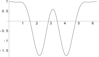
Figure 14.5 shows the first four basis functions from one common set used for the discrete cosine transform:
![]()
Figure 14.5. The first four basic cosine functions used in Fourier series expansions: cos(x), cos(2x), cos(3x) and cos(4x).

Another version uses the similar version with a different value at the endpoint:
![]()
Each of these transforms also has an inverse operation. This is useful because many mathematical operations are easier to do “in the frequency space”. That is, the amount of energy in each frequency in the data is computed by constructing the transforms. Then some basic operations are done on the frequency coefficients, and the data is then restored with the inverse FFT or DCT.
Figure 14.9 shows the 64 different two-dimensional cosine functions used as the basis functions to model 8 × 8 blocks of pixels for JPEG and MPEG compression.
Smoothing data is one operation that is particularly easy to do with the FFT and DCT— if the fundamental signal is repetitive. Figure 14.10 shows the four steps in smoothing data with the Fourier transform. The first graph shows the noisy data. The second shows the absolute value of the Fourier coefficients. Both y4 and y251 are large despite the effect of the noise. The third graph shows the coefficients after all of the small ones are set to zero. The fourth shows the reconstructed data after taking the inverse Fourier transform. Naturally, this solution works very well when the signal to be cleaned can be modeled well by sine and cosine functions. If the data doesn't fit this format, then there are usually smaller distinctions between the big and little frequencies making it difficult to remove the small frequencies.
Figure 14.9. The 64 two-dimensional basis functions used in the two-dimensional discrete cosine transform of an 8 × 8 grid of pixels. The intensity at each particular point indicates the size of the function.

Figure 14.10. The four steps in smoothing noisy data with the FFT. The first graph shows the data; the second, the result of computing the FFT; the third, data after small values are set to zero; and fourth, the final result.

14.7. Hiding Information with FFTs and DCTs
Fourier transforms provide ideal ways to mix signals and hide information by changing the coefficients. A signal that looks like cos(4πx) can be added by just increasing the values of y4 and y251. The more difficult challenge is doing this in a way that is hard to detect and resistant to changes to the file that are either malicious or incidental.
Here's an example. Figure 14.11 shows the absolute value of the first 600 coefficients from the Fourier transform of the voice signal shown in Figure 14.3. The major frequencies are easy to identify and change if necessary.
Figure 14.11. The first 600 coefficients from the Fourier transform of Figure 14.3.

A simple watermark or signal can be inserted by changing setting y300 = 100000. The result after taking the inverse transform looks identical to Figure 14.3 at this level of detail. The numbers still range from −30,000 to 30,000. The difference, though small, can be seen by subtracting the original signal from the watermarked one. Figure 14.12 shows that the difference oscilliates between 750 and −750 with the correct frequency.
Figure 14.12. The result of subtracting the original signal shown in Figure 14.3 from the signal with an inflated value of y300.

14.7.1. Tweaking a Number of Coefficients
Ingemar Cox, Joe Kilian, Tom Leighton and Talal Shamoon [CKLS96] offer a novel way to hide information in an image or sound file by tweaking the k largest coefficients of an FFT or a DCT of the data. Call these {y1, y2, … yk−1}. The largest coefficients correspond to the most significant parts of the data stream. They are the frequencies that have the most “energy” or that do the most for carrying the information about the final image.
Cox and colleagues suggest that hiding the information in the largest coefficients may sound counterintuitive, but it is the only choice. At first glance, the most logical place to hide the data is in the noise— that is, the smallest coefficients. But this noise is also the most likely to be modified by compression, printing, or using a less than perfect conversion process. The most significant parts of the signal, on the other hand, are unlikely to be damaged without damaging the entire signal.
This philosophy has many advantages. The data is spread out over numerous data elements. Even if several are changed or deleted, the information can be recovered. Cox and colleagues demonstrate that the images carrying this watermark can survive even after being printed and scanned in again. Of course, the bandwidth is also significantly smaller than other solutions like tweaking the least signficant bit.
Their algorithm uses these steps:
- Use a DCT or FFT to analyze the data.
- Choose the k largest coefficients and label them {y0, y1, y2, … yk −1} for simplicity. The smaller coefficients are ignored. The first coefficients representing the smallest frequencies will often be in this set, but it isn't guaranteed.Another solution is to order the
coefficients according to their visual significance. Figure 14.13 shows a zig-zag ordering used to choose the coefficients with the lowest frequencies from a two-dimensional transform. The
JPEG and MPEG algorithms use this approach to eliminate unnecessary coefficients. Some authors suggest skipping the first
l coefficients in this ordering because they have such a big influence on the image. [PBBC97] Choosing the next k coefficients produces candidates that are important to the description of the image but not too important.
Figure 14.13. Another solution is to order the coefficients in significance. This figure shows the popular zig-zag method to order coefficients from a two-dimensional transform. The ones in the upper lefthand corner correspond to the lowest frequencies and are thus the most significant for the eye.

- Create a k-element vector, {b1, b1, b2,…bk−1}, to be hidden. These can be either simple bits or more information rich real numbers. This information will not be recovered intact in all cases, so it should be thought of more as an identification number, not a vector of crucial bits.
- Choose α, a coefficient that measures the strength of the embedding process. This decision will probably be made via trial and error. Larger values are more resistant to error, but they also introduce more distortion.
- Encode the bit vector in the data by modifying the coefficients with one of these functions they suggest:
-
- Compute the inverse DCT or FFT to produce the final image or sound file.
The existence of the embedded data can be tested by reversing the steps. This algorithm requires the presence of the original image, a problem that severely restricts its usefulness in many situations. The steps are:
- Compute the DCT or FFT of the image.
- Compute the DCT or FFT of the original image without embed ded data.
- Compute the top k coefficients.
- Use the appropriate formula to extract the values of αbi.
- Use the knowledge of the distribution of the random elements, bi, to normalize this vector. That is, if the values of bi are real numbers chosen from a normal distribution around .5, then determine which value of α moves the average to .5. Remove α from the vector through division.
- Compare the vector of {b0, b1, b2, … bk−1} to the other known vectors and choose the best match.
The last step for identifying the “watermark” is one of the most limiting for this particular algorithm. Anyone searching for it must have a database of all watermarks in existence. The algorithm usually doesn't identify a perfect match because roundoff errors add imprecision even when the image file is not distorted. The process of computing the DCTs and FFTs introduces some roundoff errors and encapuslating the image in a standard 8-bit or 24-bit format adds some more. For this reason, the best we get is the most probable match.
This makes the algorithm good for some kinds of watermarks but less than perfect for hidden communication. The sender and receiver must agree on both the cover image and some code book of messages or watermarks that will be embedded in the data.
If these restrictions don't affect your needs, the algorithm does offer a number of desirable features. Cox and colleagues tested the algorithm with a number of experiments that proved its robustness. They began with several 256 × 256 pixel images, distorted the images and then tested for the correct watermark. They tried shrinking the size by a factor of 1/2, using heavy JPEG compression, deleting a region around the outside border, and dithering it. They even printed the image, photocopied it, and scanned it back in without removing the watermark. In all of their reported experiments, the algorithm identified the correct watermark, although the distortions reduced the strength.
The group also tested several good attacks that might be mounted by an attacker determined to erase the information. First, they tried watermarking the image with four new watermarks. The final test pulled out all five, although it could not be determined which were the first and the last. Second, they tried to average together five images created with different watermarks and found that all five could still be identified. They indicate, however, that the algorithm may not be as robust if the attacker were to push this a bit further, say by using 100 or 1000 different watermarks.
14.7.2. Removing the Original from the Detection Process
Keeping the original unaltered data on hand is often unacceptable for applications like watermarking. Ideally, an average user will be able to extract the information from the file without having the original available. Many of the watermarking applications assume that the average person can't be trusted with unwatermarked data because they'll just pirate it.
A variant of the previous algorithm from Cox et al. does not require the original data to reveal the watermark. A. Piva, M. Barni, F. Bartolini, and V. Cappellini produced a similar algorithm that sorts the coefficients to the transform in a predictable way. Figure 14.13, for instance, shows a zig-zag pattern for ordering the coefficients from a two dimensional transform according to their rough frequency. If this solution is used, there is no need to keep the original data on hand to look for the k most significant coefficients. Many other variants are emerging.
14.7.3. Tempering the Wake
Inserting information by tweaking the coefficients can sometimes have a significant effect on the final image. The most fragile sections of the image are the smooth, constant patches like pictures of a clear, blue, cloudless summer sky. Listeners can often hear changes in audio files with pure tones or long quiet segments. Data with rapidly changing values mean there is plenty of texture to hide information. Smooth, slowly changing data means there's little room. In this most abstract sense, this follows from information theory. High entropy data is a high bandwidth channel. Low entropy data is a low bandwidth channel.
Some algorithms try to adapt the strength of a watermark to the underlying data by adjusting the value of α according to the camouflaging data. This means the strength of the watermark becomes a function of location (αi,j) in images and of time (αt) in audio files.
There are numerous ways to calculate this value of α, but the simplest usually suffice. Taking a window around the point in space or time and averaging the deviation from the mean is easy enough. [PBBC97] More sophisticated studies of the human perception system may be able to provide a deeper understanding of how our eyes and ears react to different frequencies.
14.8. Wavelets
Many of the algorithms use sines and cosines as the basis for constructing models of data, but there is no reason why the process should be limited to them alone. In recent years, researchers began devoting new energy to exploring how strange and different functions can make better models of data– a field the researchers call wavelets. Figure 14.14 shows one popular wavelet function, the Meyer ψ function.
Figure 14.14. The Meyer ψ function.

Some of the steganography detection algorithms examine the statistics of wavelet decompositions. See Section 17.6.1.
Wavelet transforms construct models of data in much the same way Fourier transforms or Cosine transforms do — they compute coefficients that measure how much a particular function behaves like the underlying data. That is, the computation finds the correlation. Most wavelet analysis, however, adds an additional parameter to the mix by changing both the frequency of the function and the location or window where the function is non-zero. Fourier transforms, for instance, use sines and cosines that are defined from −∞ to +∞. Wavelet transforms restrict the influence of each function by sending the function to zero outside a particular window from a to b.
Using these localized functions can help resolve problems that occur when signals change over time or location. The frequencies in audio files containing music or voice change with time and one of the popular wavelet techniques is to analyze small portions of the file. A wavelet transform of an audio file might first use wavelets defined between 0 and 2 seconds, then use wavelets defined between 2 and 4 seconds, etc. If the result finds some frequencies in the first window but not in the second, then some researchers say that the wavelet transform has “localized” the signal.
Roz Chast's collection, Theories of Everything lists books “not by the same author” including Nothing But Cosines.
The simplest wavelet transforms are just the DCT and FFT computed on small windows of the data. Splitting the data into smaller windows is just a natural extension of these algorithms.
More sophisticated windows use multiple functions defined at multiple sizes in a process called multi-resolution analysis. The easiest way to illustrate the process is with an example. Imagine a sound file that is 16 seconds long. In the first pass, the wavelet transform might be computed on the entire block. In the second pass, the wavelet transform would be computed on two blocks between 0 and 7 seconds and between 8 and 15 seconds. In the third pass, the transform would be applied to the blocks 0 to 3,4 to 7, 8 to 11, and 12 to 15. This is three stage, multi-resolution analysis. Clearly, it is easier to simply divide each window or block by two after each stage, but there is no reason why extremely complicated schemes with multiple windows overlapping at multiple sizes can't be dreamed up.
Multiple resolution analysis can be quite useful for compression, a topic that is closely related to steganography. Some good wavelet-based compression functions use this basic recursive approach:
- Use a wavelet transform to model the data on a window.
- Find the largest and most significant coefficients.
- Construct the inverse wavelet transform for these large coefficients.
- Subtract this version from the original. What is left over is the smaller details that couldn't be predicted well by the wavelet transform. Sometimes this is significant and sometimes it isn't.
- If the differences are small enough to be perceptually insignificant, then stop. Otherwise, split the window into a number of smaller windows and recursively apply this same procedure to the leftover noise.
This recursive, multi-resolution analysis does a good job of compressing many images and sound files. The wider range of choices in functions means that the compression can be further tuned to extract the best performance. There are many different wavelets available and some are better at compressing some files than others. Choosing the best one is often as much an art as a science.
In some cases, steganographers suggest that the choice of the function can also act like a key if only the sender and the receiver know the particular wavelet.
It is not possible to go into the wavelet field in much depth here because it is more complex and not much of this complexity affects the ability to hide information.
Most of the same techniques for hiding information with DCTs and DFTs work well with DWTs. In some cases, they outperform the basic solutions. It is not uncommon to find that information hidden with DWTs does a better job of surviving wavelet-based compression algorithms than information hidden with DCTs or DFTs. [XBA97] Using the same model for compression and information hiding works well. Of course, this means that an attacker can just choose a different compression scheme or compress the file with a number of schemes in the hope of foiling one.
Are highly tuned wavelets more or less stable for information encoding? That is, can a small change in a coefficient be reliably reassembled later, even after printing and scanning? In other words, how large must the α term be?
14.9. Modifications
The basic approach to hiding information with sines, cosines or other wavelets is to transform the underlying data, tweak the coefficients, and then invert the transformation. If the choice of coefficients is good and the size of the change is manageable, then the result is pretty close to the original.
There are a number of variations on the way to choose the coefficients and encode some data in the ones that are selected. Here are some of the more notable:
- Identify the Best Areas Many algorithms attempt to break up an image or sound file and identify the best parts for hiding the information. Smooth, stable regions turn mottled or noisy if coefficients are changed even a small amount. Multi-resolution wavelet transforms are a good tool for identifying these regions because they recursively break up an image until a good enough model is found. Smooth, stable sections are often modeled on a large scale, while noisy, detailed sections get broken up multiple times. The natural solution is to hide the information in the coefficients that model the smallest, most detailed regions. This confines the changes to the edges of the objects in images or the transitions in audio files, making it more difficult for the human perception system to identify them. [AKSK00]
- Quantize the Coefficients to Hide Information Many of the transform hiding methods hide information by adding in a watermark vector. The information is extracted by comparing the coefficients with all possible vectors and choosing the best match. This may be practical for small numbers of watermarks, but it doesn't work well for arbitrary blocks of information. A more flexible solution is to tweak the coefficients to hide individual bits. Let Q be some quantization factor. An arbitrary coefficient, yi, is going to fall between aQ ≤ yi ≤ (a + 1)Q for some integer, a. To encode a bit, round off yi to the value where the least significant bit of a is that bit. For example, if the bit to be encoded is zero and a = 3, then set yi = (a + 1)Q = 4Q. [KH98] Any recipient would extract a bit from yi by finding the closest value of aQ. If the transform process is completely accurate, then there will be some integer where aQ = yi. If the transform and inverse transform introduce some rounding errors, as they often do, then yi should still be close enough to some value of aQ— if Q is large enough. The value of Q should be chosen with some care. If it is too large, then it will lead to larger changes in the value of yi. If it is too small, then it may be difficult to recover the message in some cases when error intrudes. Deepa Kundur and Dimitrios Hatzinakos describe a quantization-based watermark that also offers tamper detection. [KH99] This mechanism also offers some ability to detect tampering with the image or sound file. If the coefficients are close to some value of aQ but not exactly equal to aQ, then this might be the result of some minor changes in the underlying file. If the changes are small, then the hidden information can still be extracted. In some cases, the tamper detection can be useful. A stereo or television may balk at playing back files with imperfect watermarks because they would be evidence that someone was trying to destroy the watermark. Of course it could also be the result of some imperfect copying process.
- Hide the Information in the Phase The Discrete Fourier Transform produces coefficients with a real and an imaginary value. These complex values can also be imagined in polar coordinates as having a magnitude and an angle. (If yi = a + bi, then a = mcos(θ) and b = msin(θ), where m is the magnitude and θ is the angle.) Many users of the DFT feel that the transform is more sensitive to changes made in the angles of the coefficient than changes made in the magnitude of the coefficients. [RDB96, LJ00] This method is naturally adaptive to the size of the coefficients. Small values are tweaked a small amount if they're rotated θ + ψ degrees. Large values are tweaked a large amount. Changing the angle this way requires a bit of attention to symmetry. When the input to a DFT are real values, as they almost are in steganographic examples, then the angles are symmetric. This symmetry must be preserved to guarantee real values will emerge from the inverse transform. Let θi,j stand for the angle of the coefficient (i,j). If ψ is added to θi,j, then − ψ must be added to θm − i, n − j, where (m, n) are the dimensions of the image.
14.10. Summary
Spreading the information over a number of pixels or units in a sound file adds more security and intractability. Splitting each bit of information into a number of pieces and distributing these pieces throughout a file reduces the chance of detection and increases resistance to damage. The more the information is spread throughout the file, the more redundancy blocks attacks.
Many solutions use well-understood software algorithms like the Fourier transform. These tools are usually quite popular in techniques for adding watermarks because many compression algorithms use the same tools. The watermarks are usually preserved by compression in these cases because the algorithms use the same transforms.
- The Disguise Informationis spread throughout a file by adding small changes to a number of data elements in the file. When all of the small changes are added up, the information emerges.
- How Secure Is It? The changes are small and distributed so they can be more secure than other solutions. Very distributed information is resistant to attack and change because an attacker must destroy enough of the signal to change it. The more places the information is hidden, the harder it is for the attacker to locate it and destroy it. The system can be made much more secure by using a key to create a pseudo-random bit stream that is added into the data as it is mixed into the mix. Only the person with the key can remove this extra encryption.
- How to Use It In the most abstract sense, just choose a number of locations in the file with a pseudo-random bit stream, break the data into little parts, and add these parts into all of the locations. Recover the message by finding the correct parts and adding them together. This process is very efficient if it is done with a fast Fourier transform. In these cases, the data can be hidden by tweaking the coefficients after the transform. This can add or subtract different frequency data.
Further Reading
Using wavelets, cosines or other functions to model sound and image data is one of the most common strategies for watermarking images today. There are too many good papers and books to list all of them. Some suggestions are:
- Digital Watermarking by Ingemar Cox, Matthew L. Miller and Jeffrey A. Bloom is a great introduction to using wavelet techniques to embed watermarks and hide information. The 2007 edition is broader and it includes a good treatment of steganography and steganalysis. [CMB02,CMB07]
- The proceedings of the International Workshop on Digital Watermarking are invaluable sources that track the development of steganography using wavelets and other functional decomposition. [PK03, KCR04, CKL05, SJ06]
- A good conference focused on watermarking digital content is the Security, Steganography, and Watermarking of Multimedia Contents. [DW04, DW05]
- Jessica J. Fridrich, Miroslav Goljan, Petr Lisonek and David Soukal discuss the use of Michael Luby's LT Codes as a foundation for building better versions of perturbed quantization. These graph-based codes can be faster to compute than the matrix-based solutions. [Lub02,FGLS05]